Research on Information Identification of Chaotic Map with Multi-Stability

Abstract

Influenced by the rapid development of artificial intelligence, the identification of chaotic systems with intelligent optimization algorithms has received widespread attention in recent years. This paper focuses on the intelligent information identification of chaotic maps with multi-stability properties, and an improved sparrow search algorithm is proposed as the identification algorithm. Numerical simulations show that different initial values can lead to the same dynamic behavior, making it impossible to stably and accurately identify the initial values of multi-stability chaotic maps. An identification scheme without considering the initial values is proposed for solving this problem, and simulations demonstrate that the proposed method has the highest identification precision among seven existing intelligent algorithms and a certain degree of noise resistance. In addition, the above research reveals that chaotic systems with multi-stability may have more potential applications in fields such as secure communication.

1. Introduction

Over the past few decades, chaos theory research has attracted increasing attention. Due to its special properties such as ergodicity, randomness, and sensitivity to initial values [1], chaos has a wide range of applications in fields like electronic information, artificial intelligence, biology, and materials science [2,3,4,5,6,7,8]. In general, it is not difficult to collect the data in respect of chaotic behavior in nonlinear systems, but it is not possible to clearly deduce the exact mathematical model of the chaos phenomenon. Without prior information, how to accurately identify various types of system parameter through the collected data is the key to utilizing and controlling chaos [9,10].

Due to the rapid development of artificial intelligence technology, the introduction of intelligent optimization algorithms for the parameter identification of chaotic systems has become a hot topic in recent years. This method is simple and robust, and it is not sensitive to the considered system. So far, multiple intelligent optimization algorithms have been proposed for identifying the parameters of chaotic systems. For example, Xu et al. [11] proposed a hybrid flower pollination algorithm for the parameter identification of a Lorenz system, Rössler system, and other classical chaotic systems. Gupta et al. [12] and Hu et al. [13] designed two improved artificial bee colony algorithms to study the parameter identification of fractional-order nonlinear systems, and simulations demonstrated the good identification display. Yousri et al. [14] reported the chaotic whale optimization variants to be applied in the parameter identification of a permanent magnet synchronous motor with hyperchaotic behavior. The results show that the algorithm combined with a logistic map has the best performance. In addition, the JAYA algorithm [15], differential evolution algorithm [16], particle swarm optimization algorithm [17], bird swarm algorithm [18], sunflower optimization algorithm [19], butterfly optimization algorithm [20], and other intelligent optimization algorithms are utilized to identify the parameters of nonlinear systems with chaotic behavior.

Until recently, most reports for the parameter identification of chaotic systems have only focused on the system parameters, while the identification research for the initial values is not enough [21,22]. As a matter of fact, the initial value also has an important impact on the generation behavior of the chaotic system, so it is necessary to conduct in-depth research on initial value identification.

Recently, a new dynamical system called a multi-stability chaotic system was discovered, and it has been reported in many papers [23,24,25,26]. It is different from regular chaotic systems; any imperfect identification of system parameters and initial values not only causes time-series with different quantities, but also with different qualities. This means that tiny changes in the initial values may result in different chaotic attractors, especially in discrete chaotic maps [27,28,29].

To sum up, these issues have driven us to further study the identification of system parameters and initial values in multi-stability chaotic maps. In order to obtain more accurate results, we introduce the sparrow search algorithm (SSA) [30], which has been proven to have better performance than some intelligent optimization algorithms like particle swarm optimization, the differential evolution algorithm, the genetic algorithm, etc. A new improved sparrow search algorithm (ISSA) has also been designed for information identification.

The remainder of this paper is organized as follows. The framework for the information identification of chaotic maps is introduced in Section 2. Section 3 presents the proposed ISSA. Numerical simulations with and without initial values are given in Section 4 and Section 5, respectively. Finally, Section 6 summarizes the conclusions and presents the prospects for future work.

2. Information Identification of Chaotic Map

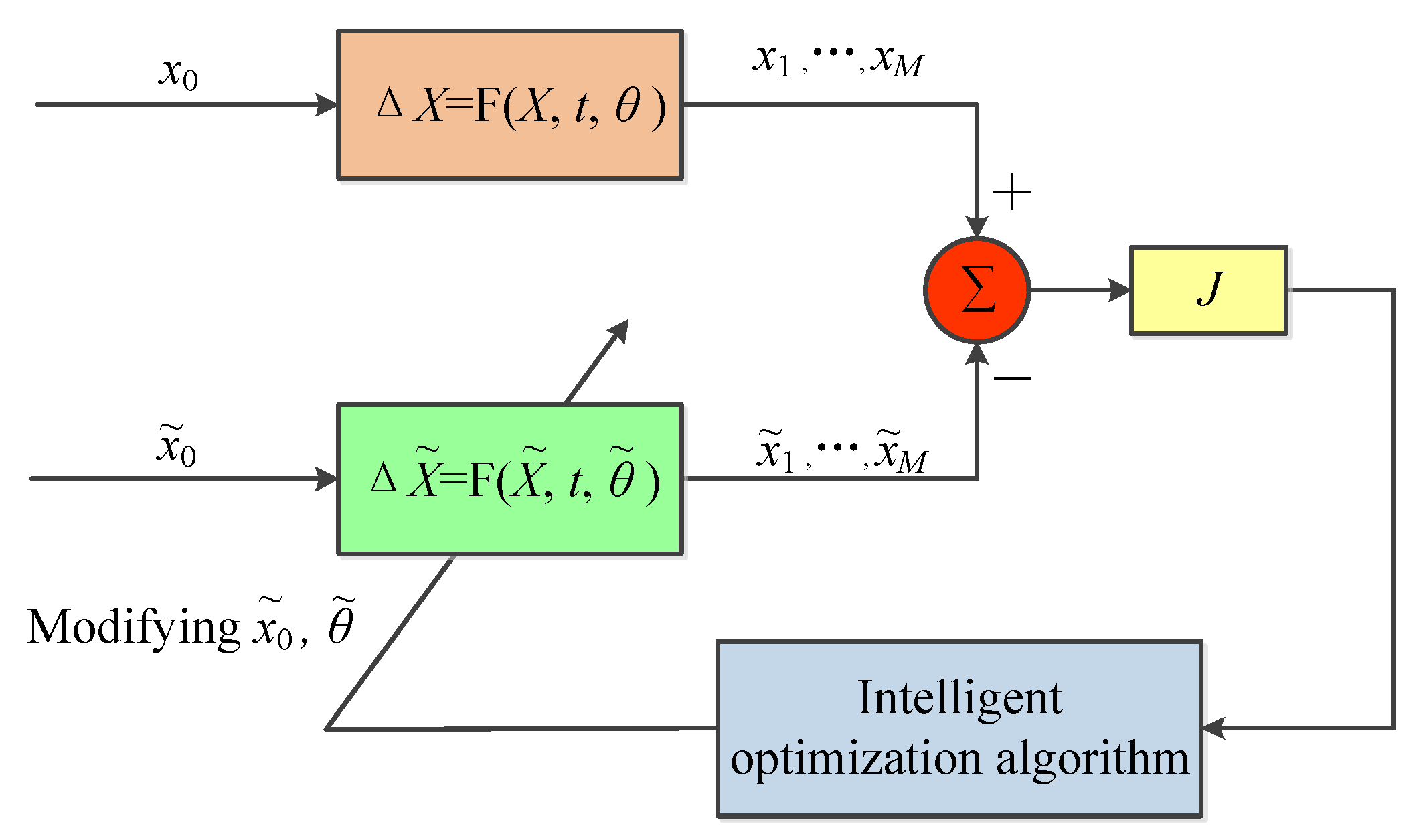
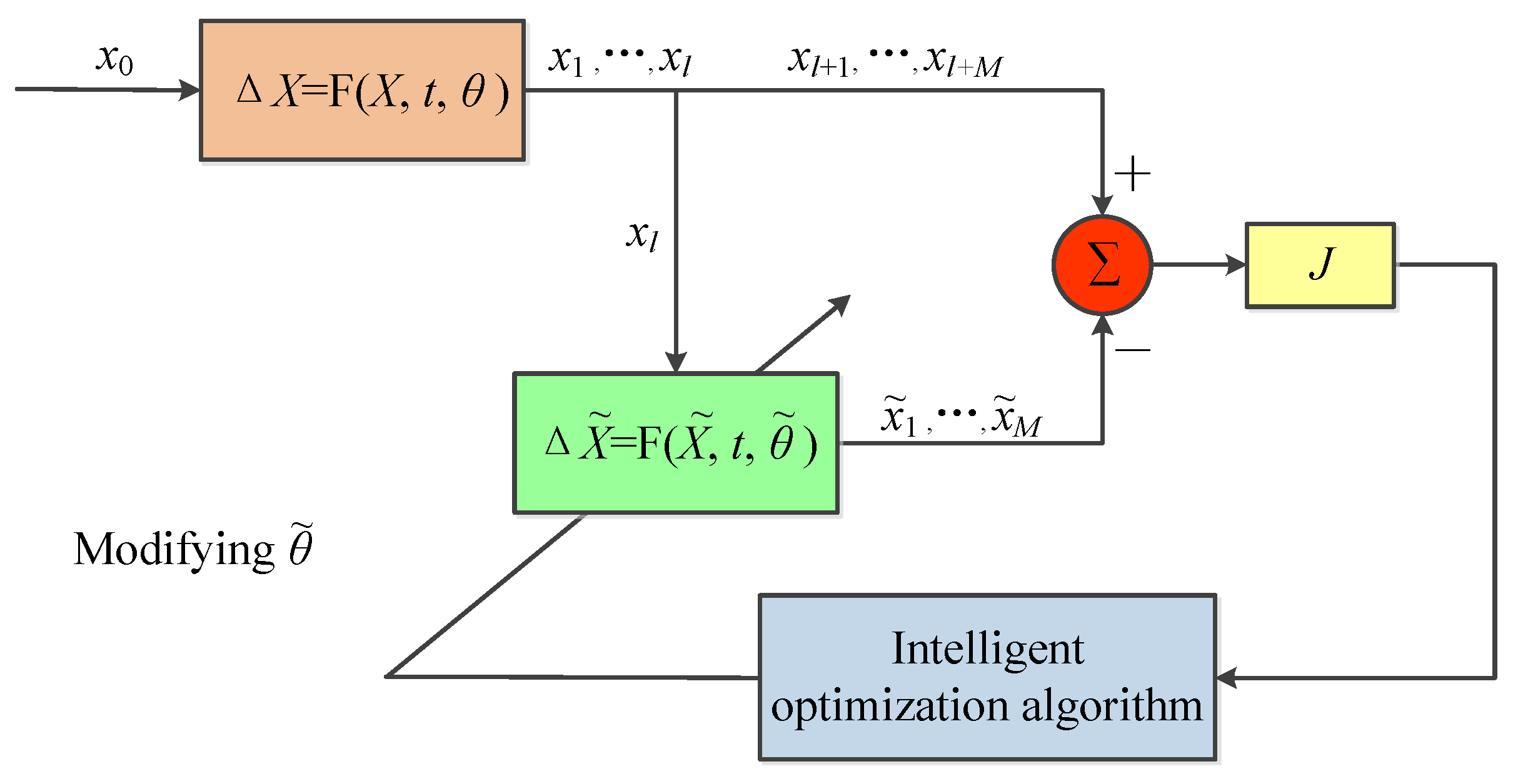
For chaotic maps utilized in practical applications, the most crucial information is the system parameters and initial values, as they directly affect the dynamic behavior generated by the system. In this paper, the basic framework for the parameter and initial value identification of chaotic maps is shown in Figure 1. According to this figure, the identification process is regarded as a typical optimization problem.

The original chaotic map is

$$\Delta X=\mathrm{F}(X,t,\theta ),$$

(1)

where {$X=x_1,x_2,\dots ,x_M$} denotes the state vector of the original system and M is the number of samples in the identification. $x_0$ is the initial value and t is the iteration number of the chaotic map. {$\theta ={\theta }_1,{\theta }_2,\dots ,{\theta }_D$} represents the system parameters and D is the number of system parameters. The character with the “∼” symbol above it represents the various information of the identified system, and the meaning of this information corresponds to the original system.

Symbol J is the goal of the identification problem, which is generally set as the mean squared error between the original and the identification time series

$$J=\frac{1}{M}\sum _{t=1}^M{(X_t-{\tilde{X}}_t)}^2.$$

(2)

Therefore, the information identification problem is regraded as a multi-dimensional optimization problem with an objective function J. The optimization process involves continuously modifying the initial values and system parameters through the intelligent optimization algorithm to make the value of target J close to 0, thereby accurately identifying the key information of the original system.

3. The Proposed Intelligent Optimization Algorithm

In this study, SSA was selected as the optimization algorithm for information identification. In order to improve the precision, we designed an improved sparrow search algorithm (ISSA) that incorporates two new schemes; namely, inertial weight and chaotic search.

3.1. Classical Sparrow Search Algorithm

SSA is a bionics swarm intelligence optimization algorithm that simulates the group behavior of sparrows in foraging. It consists of three types of sparrow populations, i.e., producers, scroungers, and scouters, so the algorithm is mainly divided into three update steps. The producers are responsible for guiding the direction of the population and finding the foraging area, while the scroungers will always follow the producers and compete for food. The scouters are responsible for guarding the population. If a predator is found, they will issue an alarm, causing the entire population to migrate within their activity range.

We assume that the sparrow population has a total of N ($i\in [1,N]$) sparrows. The mathematical equation for updating the location of the producers is

$$Y_{i,j}(t+1)=\left\{\begin{array}{cc}{Y}_{i,j}\left(t\right)\exp \left(\frac{-i}{\alpha T}\right),\hfill & \mathrm{if}{R}_2<ST,\hfill \\ Y_{i,j}\left(t\right)+QL,\hfill & \mathrm{if}{R}_2\ge ST,\hfill \end{array}\right.$$

(3)

where t is the current generation number and T is the maximum generation number. $Y_{i,j}(·)$ is the position of the i-th sparrow in the j-th dimension solution space. $\alpha$ is a random number between 0 and 1. Q is a random number subject to the normal distribution. L is a matrix with $1\times d$ dimensions, where each element inside is 1. $R_2\in [0,1]$ and $ST\in [0.5,1]$ are the alarm value and the safety threshold, respectively. When $R_2$ exceeds the safety threshold, this indicates that the scouters have detected the predator and the entire population will migrate to other safe areas.

The mathematical equation for updating the location of the scroungers is

$$Y_{i,j}(t+1)=\left\{\begin{array}{c}Q\exp \left(\frac{Y_{\mathrm{worst}}\left(t\right)-Y_{i,j}\left(t\right)}{i^2}\right),\mathrm{if}i>N/2,\hfill \\ Y_{\mathrm{p}}(t+1)+|Y_{i,j}\left(t\right)-Y_{\mathrm{p}}(t+1)|A^{+}L,\mathrm{otherwise},\hfill \end{array}\right.$$

(4)

where $Y_{\mathrm{p}}\left(t\right)$ is the optimal position of the producers at the t-th generation, and $Y_{\mathrm{worst}}\left(t\right)$ is the global worst position at the t-generation. A is a $1\times d$ matrix with internal elements randomly set to 1 or −1, and $A^{+}=A^T{\left(A{A}^T\right)}^{-1}$. When $i>N/2$, this indicates that the i-th scrounger will fly to other areas to search for food.

Assuming that 20% of the total population of sparrows are aware of danger (scouters), the mathematical update equation is

$$Y_{i,j}(t+1)=\left\{\begin{array}{c}{Y}_{\mathrm{best}}\left(t\right)+\beta |Y_{i,j}\left(t\right)-Y_{\mathrm{best}}\left(t\right)|,\mathrm{if}{f}_i>f_g,\hfill \\ Y_{i,j}\left(t\right)+K\left[\frac{Y_{i,j}\left(t\right)-Y_{\mathrm{worst}}\left(t\right)}{f_i-f_w+ϵ}\right],\mathrm{if}{f}_i=f_g,\hfill \end{array}\right.$$

(5)

where $Y_{\mathrm{best}}\left(t\right)$ is the global worst position at the t-generation. $\beta$ is subject to the normal distribution, and K is a random number between 0 and 1; both of these are the step-size control coefficients. $f_i$ is the fitness value of the current sparrow position; $f_g$ and $f_w$ are the current global optimal fitness value and global worst fitness value, respectively. $ϵ$ is a very small constant so as to avoid zero-division error.

3.2. Improved Sparrow Search Algorithm

The ISSA attempts to incorporate inertial weight and chaotic searching into the classical SSA to enhance the algorithm’s ability to solve local optimal dilemmas.

First, a special numerical factor called the inertial weight is added to the producer’s update equation. This will adjust adaptively based on the current fitness value and global optimal fitness value of sparrows, and gradually decrease with the increase in generation. If the current position of the sparrow is far from the optimal position, the decrease trend of the inertial weight will slow down; otherwise its value will rapidly decrease. Therefore, Equation (3) is changed to

$$Y_{i,j}(t+1)=\left\{\begin{array}{cc}w\left(t\right)Y_{i,j}\left(t\right)\exp \left(\frac{-i}{\alpha T}\right),\hfill & \mathrm{if}{R}_2<ST,\hfill \\ w\left(t\right)Y_{i,j}\left(t\right)+QL,\hfill & \mathrm{if}{R}_2\ge ST,\hfill \end{array}\right.$$

(6)

and the inertial weight is defined as

$$w\left(t\right)=(w_{max}-w_{min})\exp (-10\frac{f_i}{f_g}){\left(\frac{t}{T}\right)}^2+w_{min},$$

(7)

where $w_{max}$ and $w_{min}$ are set to 1.5 and 0.6, respectively.

Next, a novel search strategy called chaotic searching is proposed. This is intended to seek in a certain range according to the global optimal position at the current generation, aiming to guide the algorithm to jump out of a local optimum. The sparrow position in the chaotic search is updated as

$$Y\left(t\right)=(Y_{\mathrm{best}}\left(t\right)-a{Y}_{\mathrm{best}}\left(t\right))+[(Y_{\mathrm{best}}\left(t\right)+a{Y}_{\mathrm{best}}\left(t\right))-(Y_{\mathrm{best}}\left(t\right)-a{Y}_{\mathrm{best}}\left(t\right))]x_n,$$

(8)

where a determines the search scope and $a\in (0,1)$. $x_n$ is generated according to the logistic-logistic chaotic system (LLS) [31], and its mathematical equation is

$$x\left(n\right)=\mu x_{n-1}(1-x_{n-1})\times 2^{14}-\mathrm{floor}(\mu x_{n-1}(1-x_{n-1})\times 2^{14}),$$

(9)

where $\mu$ is set to $\mu =5$ here. The LLS has a high Lyapunov exponent, so its randomness is very strong. Moreover, the values of the sequence generated are also evenly distributed between 0 and 1, which is very conducive to the search process.

Finally, the execution process of the ISSA is presented in Algorithm 1.

Algorithm 1 Pseudo code of ISSA

1: Initialize N, $ST$, T, and a 2: Evaluate the fitness value of each particle; find the best and the worst sparrow position 3: while  $t<T$ do 4:    for i = 1 : the number of producers do 5:        Update new position by Equation (6) 6:    end for 7:    for i = the number of producers +1 : N do 8:        Update new position by Equation (4) 9:    end for 10:    for i = 1 : the number of producers do 11:        Update new position by Equation (5) 12:    end for 13:    Execute chaotic search according to Equation (8) 14:    Preserve better sparrow’s position 15:    t = t + 1 16: end while

4. Identification of Initial Values and System Parameters

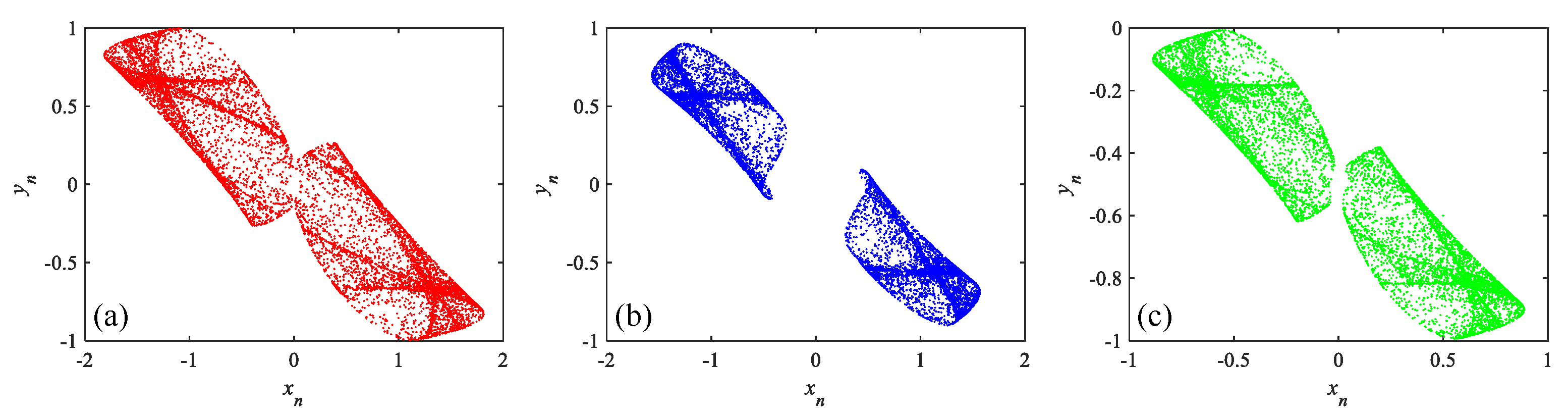
In this section, multiple intelligent optimization algorithms are introduced to directly identify initial values and system parameters using the approach shown in Figure 1. The identification system considered comprises three memristive hyperchaotic maps with multi-stability properties.

4.1. Identification Systems

The three identification systems comprise a quadratic discrete memristor (QDM) system, absolute value discrete memristor (ADM) system, and sinusoidal discrete memristor (SDM) system [29]. Their formulas are derived as follows.

The mathematical equation of the QDM system is

$$\left\{\begin{array}{c}{x}_{n+1}=k(y_n^2-1)x_n,\hfill \\ y_{n+1}=x_n+y_n,\hfill \end{array}\right.$$

(10)

the mathematical equation of the ADM system is

$$\left\{\begin{array}{c}{x}_{n+1}=k\left(\right|y_n|-1)x_n,\hfill \\ y_{n+1}=x_n+y_n,\hfill \end{array}\right.$$

(11)

and the mathematical equation of the SDM system is

$$\left\{\begin{array}{c}{x}_{n+1}=ksin\left(\pi y_n\right)x_n,\hfill \\ y_{n+1}=x_n+y_n,\hfill \end{array}\right.$$

(12)

where k is the system parameter. All of the systems are hyperchaotic maps composed of different nonlinear memristives, and they have multi-stability characteristics controlled by the initial values ($x_0$, $y_0$). Here, the initial state settings of these three systems are listed in

Table 1. Initial states of the identification systems.

System	System Parameter	Initial Value
QDM	$k=1.78$	$x_0=-0.5, y_0=0.5$
ADM	$k=2.3$	$x_0=-0.8, y_0=0.6$
SDM	$k=1.84$	$x_0=0.5, y_0=-0.6$

, and all systems exhibit hyperchaos behavior, as plotted in Figure 2.

4.2. Numerical Simulation

Numerical simulations were carried out in systems (10), (11), and (12), and the information that needed to be identified is given in Table 1. To verify the advantages and effectiveness of the proposed ISSA, six other intelligent algorithms, i.e., the differential evolution (DE) algorithm [32], particle swarm optimization (PSO) algorithm [33], artificial bee colony (ABC) algorithm [34], bird swarm algorithm (BSA) [35], and JAYA [36], were used for the comparison. The detailed parameter settings for the intelligent optimization algorithm are shown in

Table 2. Parameter settings of different intelligent optimization algorithms.

Algorithm	Parameter Setting
DE	$CR=F=0.6$
PSO	$c_1=c_2=2, {\omega }_{min}=0.4, {\omega }_{max}=0.9$
ABC	$limit=100$
BSA	$C=S=1.5, a_1=a_2=1, FQ=3, P\in [0.8, 1], FL\in [0.5, 0.9]$
JAYA	-
SSA	$ST=0.8$
ISSA	$ST=0.8, a=0.6$

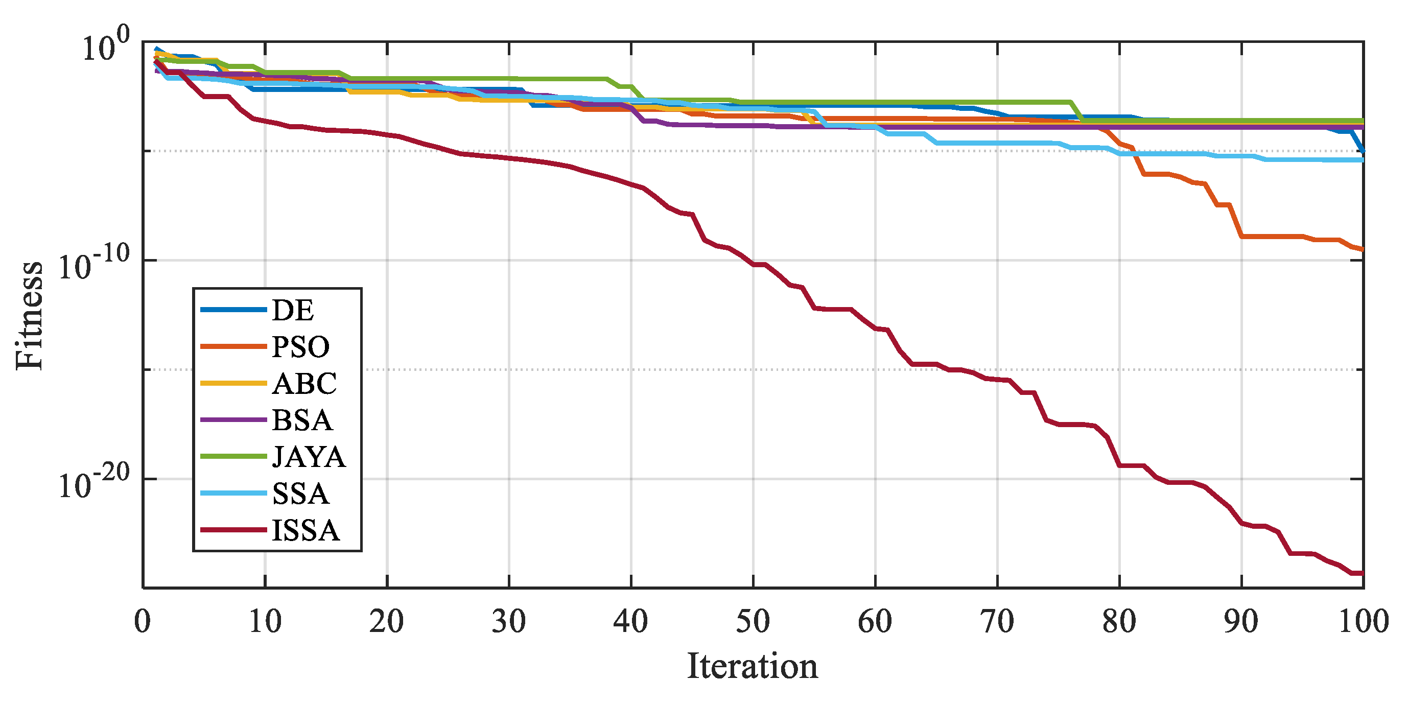
. The number of samples in the identification was set to $M=3$, and the population size of all algorithms was fixed to $N=40$. According to the settings given in Table 1, the individual particle search range in all algorithms was set to [−3, 3]. The algorithm maximum generation was $T=100$, and we performed over 30 consecutive algorithm runs to eliminate the stochastic nature of the algorithms. Simulations were based on MATLAB 2020a on an Intel(R) Core(TM) i7-6700 CPU at 3.40 GHz with 8 GB RAM.

The identification results for QDM are shown in

Table 3. Initial value and system parameter identification results for QDM.

Algorithm	Min J	Average J	Standard Deviation	Accurate Identification
DE	1.0596 $\times {10}^{-9}$	7.6312 $\times {10}^{-7}$	1.1302 $\times {10}^{-6}$	$k=1.7800, x_0=-0.5000,y_0=0.5000$  $k=1.7800, x_0=-0.6514, y_0=0.6514$
PSO	3.6528 $\times {10}^{-14}$	6.1925 $\times {10}^{-11}$	1.6995 $\times {10}^{-10}$	$k=1.7800, x_0=-0.5000, y_0=0.5000$  $k=1.7800, x_0=-0.6514, y_0=0.6514$  $k=1.7800, x_0=1.1514, y_0=-1.1514$
ABC	1.2452 $\times {10}^{-5}$	1.3061 $\times {10}^{-3}$	1.2951 $\times {10}^{-3}$	-
BSA	7.1560 $\times {10}^{-14}$	1.8623 $\times {10}^{-3}$	1.1445 $\times {10}^{-2}$	$k=1.7800,x_0=-0.5000, y_0=0.5000$  $k=1.7800, x_0=-0.6514, y_0=0.6514$  $k=1.7800, x_0=1.1514, y_0=-1.1514$
JAYA	7.2978 $\times {10}^{-5}$	9.1129 $\times {10}^{-4}$	8.5444 $\times {10}^{-4}$	-
SSA	3.3176 $\times {10}^{-15}$	1.1539 $\times {10}^{-5}$	8.1394 $\times {10}^{-5}$	$k=1.7800, x_0=-0.5000, y_0=0.5000$  $k=1.7800, x_0=-0.6514, y_0=0.6514$  $k=1.7800, x_0=1.1514, y_0=-1.1514$
ISSA	8.2173 $\times {10}^{-32}$	2.7615 $\times {10}^{-28}$	1.5450 $\times {10}^{-27}$	$k=1.7800, x_0=-0.5000, y_0=0.5000$  $k=1.7800, x_0=-0.6514, y_0=0.6514$  $k=1.7800, x_0=1.1514, y_0=-1.1514$

. The objective function J reflects the error between the original system-generated sequence and the estimated system-generated sequence. Normally, the smaller the value, the smaller the difference between the identified information and the original information. Here, we stipulate that when the value of J is no more than $1\times {10}^{-8}$, it is determined that the information identified is accurate.

As is illustrated in Table 3, except for ABC and JAYA, all other algorithms can accurately identify the information of the original system. From the stability of the algorithm identification results, the proposed ISSA has the best performance, and PSO ranks second. However, all of these algorithms have 1 or 2 additional accurate identification results ($k=1.7800, x_0=-0.6514, y_0=0.6514$ and $k=1.7800, x_0=1.1514, y_0=-1.1514$). The reason for this may be due to the interference of the multi-stability properties, and the detailed analysis is listed in the following Section 4.3.

The identification results for QDM are listed in

Table 4. Initial value and system parameter identification results for ADM.

Algorithm	Min J	Average J	Standard Deviation	Accurate Identification
DE	2.5280 $\times {10}^{-12}$	1.5302 $\times {10}^{-7}$	5.4263 $\times {10}^{-7}$	$k=2.3000, x_0=-0.8000, y_0=0.6000$  $k=2.3000, x_0=-0.4000, y_0=0.2000$
PSO	6.8340 $\times {10}^{-14}$	9.0310 $\times {10}^{-11}$	3.0218 $\times {10}^{-10}$	$k=2.3000, x_0=-0.8000, y_0=0.6000$  $k=2.3000, x_0=-0.4000, y_0=0.2000$  $k=2.3000, x_0=1.0928, y_0=-1.2928$
ABC	1.0000 $\times {10}^{-8}$	2.1014 $\times {10}^{-4}$	4.2926 $\times {10}^{-4}$	$k=2.3000, x_0=-0.4000, y_0=0.2000$
BSA	1.7174 $\times {10}^{-14}$	3.7102 $\times {10}^{-4}$	2.5935 $\times {10}^{-2}$	$k=2.3000, x_0=-0.8000, y_0=0.6000$  $k=2.3000, x_0=-0.4000, y_0=0.2000$  $k=2.3000, x_0=1.0928, y_0=-1.2928$
JAYA	3.1510 $\times {10}^{-4}$	3.6840 $\times {10}^{-3}$	4.5653 $\times {10}^{-3}$	-
SSA	5.7673 $\times {10}^{-22}$	6.4127 $\times {10}^{-13}$	4.5076 $\times {10}^{-12}$	$k=2.3000, x_0=-0.8000, y_0=0.6000$  $k=2.3000, x_0=-0.4000, y_0=0.2000$  $k=2.3000, x_0=1.0928, y_0=-1.2928$
ISSA	3.2689 $\times {10}^{-31}$	3.2823 $\times {10}^{-29}$	8.4737 $\times {10}^{-29}$	$k=2.3000, x_0=-0.8000, y_0=0.6000$  $k=2.3000, x_0=-0.4000, y_0=0.2000$  $k=2.3000, x_0=1.0928, y_0=-1.2928$

. Similar to the results for QDM, ISSA still outperforms the other six algorithms, but it also has 2 additional accurate identification results ($k=2.3000, x_0=-0.4000, y_0=0.2000$ and $k=2.3000, x_0=1.0928,$$y_0=-1.2928$).

The identification results for SDM are presented in

Table 5. Initial value and system parameter identification results for SDM.

Algorithm	Min J	Average J	Standard Deviation	Accurate Identification
DE	1.2100 $\times {10}^{-6}$	1.4477 $\times {10}^{-3}$	2.1841 $\times {10}^{-3}$	-
PSO	2.7861 $\times {10}^{-11}$	4.0176 $\times {10}^{-3}$	8.1275 $\times {10}^{-3}$	$k=1.8400, x_0=-0.5000, y_0=0.4000$  $k=1.8400, x_0=-0.9289, y_0=0.8289$  $k=1.8400, x_0=0.6245, y_0=-0.7245$
ABC	4.8297 $\times {10}^{-6}$	4.9959 $\times {10}^{-4}$	7.6374 $\times {10}^{-4}$	-
BSA	1.7721 $\times {10}^{-12}$	6.3962 $\times {10}^{-3}$	1.1652 $\times {10}^{-3}$	$k=1.8400, x_0=0.6245, y_0=-0.7245$
JAYA	2.6764 $\times {10}^{-4}$	1.7661 $\times {10}^{-2}$	2.2592 $\times {10}^{-2}$	-
SSA	1.0565 $\times {10}^{-8}$	1.4487 $\times {10}^{-3}$	5.8847 $\times {10}^{-2}$	-
ISSA	7.0006 $\times {10}^{-26}$	8.3717 $\times {10}^{-6}$	1.2630 $\times {10}^{-4}$	$k=1.8400, x_0=-0.5000, y_0=0.4000$  $k=1.8400, x_0=-0.9289, y_0=0.8289$  $k=1.8400, x_0=0.6245, y_0=-0.7245$

. It seems that SDM generates more complex time series, and all algorithms do not perform very well in identifying its information. Among them, ISSA ranks the first, and PSO and BSA rank second and third, respectively. Although the stability of the algorithm identification results is not good, ISSA and PSO can still have 3 accurate identification results (including 2 redundant results: $k=1.8400, x_0=-0.9289, y_0=0.8289$ and $k=1.8400, x_0=0.6245, y_0=-0.7245$).

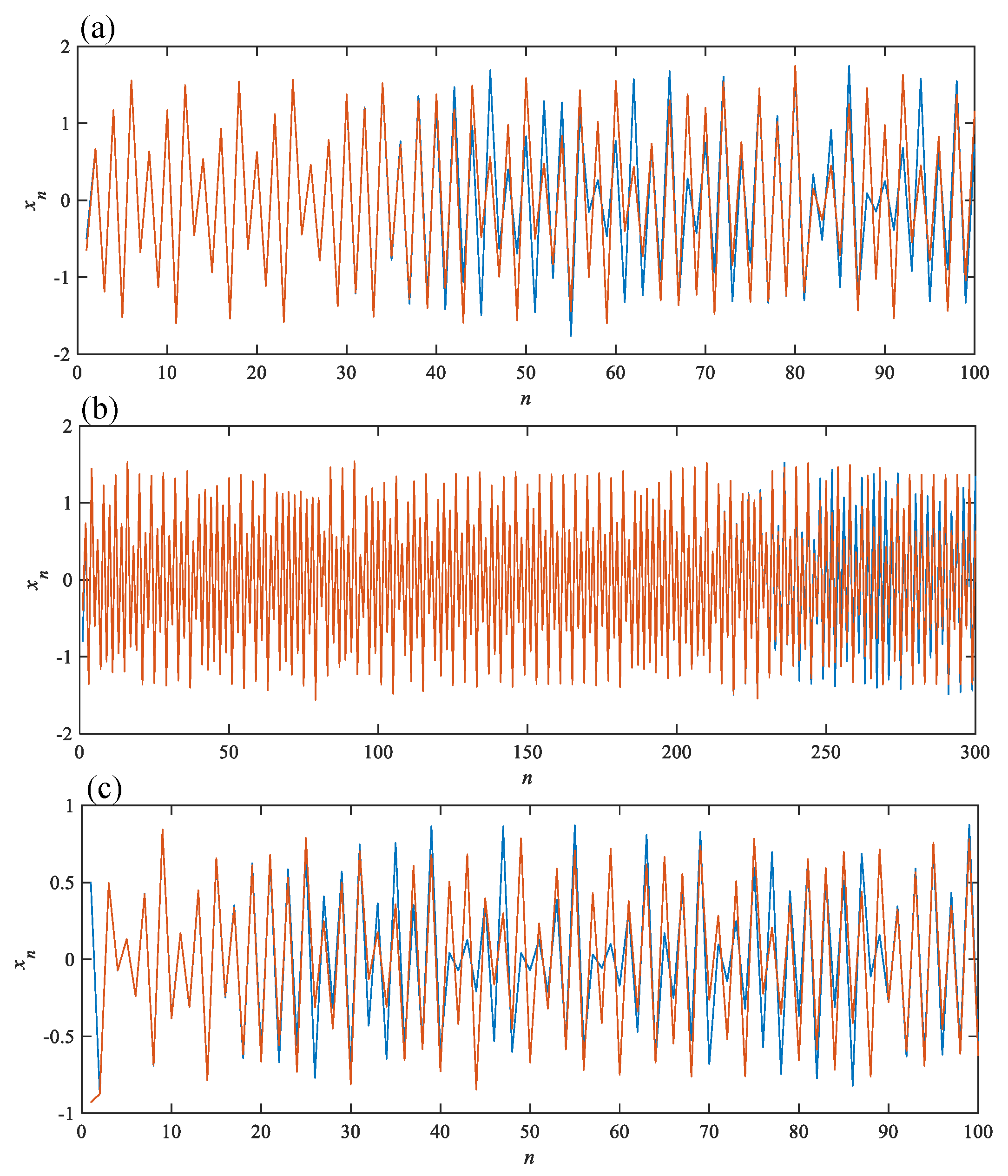
4.3. Results Analysis

According to the results of the previous section, the proposed ISSA has the highest identification precision among the seven existing algorithms. However, due to the influence of the multi-stability properties, none of the algorithms can identify the unique original information stably. The analysis of the causes of this problem is as follows.

The evolution trajectories of $x_n$ by different initial values for the three hyperchaotic memristive maps are plotted in Figure 3. From this figure, it can be seen that although the three systems evolve from completely different initial values, their dynamic behaviors are almost identical in the early stage. QDM and SDM show differences in dynamic behavior after 35 and 20 iterations of the system, respectively, while ADM does not show differences until the system performs 230 iterations. The number of sequence samples used for identification is only $M=3$ [37], which decreases the algorithm’s ability to distinguish sequence errors.

The multi-stability of the system leads to this phenomenon, i.e., different initial values may lead to the same dynamic behavior over a period of time. In the simulation using the intelligent optimization algorithm for information identification, the parameters of the identification system need to be adjusted by the error between time series. Therefore, it is impossible to conduct stable and accurate identification for initial values. This characteristic may lead to more potential application scenarios for chaotic systems with multi-stability, like secure communication, since this system, as a pseudo-random sequence generator, may make it more difficult for intelligent technology to decipher the keys.

Let us continue to study information identification for a chaotic map without multi-stability properties. Here, a famous chaotic map named the Lozi map is considered, and its equation is

$$\left\{\begin{array}{c}{x}_{n+1}=1-k|x_n+y_n|,\hfill \\ y_{n+1}=b{x}_n,\hfill \end{array}\right.$$

(13)

where system parameter b is fixed to $b=0.3$, and $k=1.5, x_0=0.1, y_0=0.1$ are set as the original information.

The results and convergence situation for the Lozi map are given in

Table 6. Initial value and system parameter identification results for Lozi map.

Algorithm	Min J	Average J	Standard Deviation	Accurate Identification
DE	4.4276 $\times {10}^{-9}$	1.2313 $\times {10}^{-5}$	2.6389 $\times {10}^{-5}$	$k=1.5000, x_0=0.1000, y_0=0.1000$
PSO	8.6821 $\times {10}^{-11}$	5.1173 $\times {10}^{-9}$	1.5569 $\times {10}^{-9}$	$k=1.5000, x_0=0.1000, y_0=0.1000$
ABC	9.4028 $\times {10}^{-6}$	1.2273 $\times {10}^{-3}$	1.2005 $\times {10}^{-3}$	-
BSA	2.9036 $\times {10}^{-13}$	2.4014 $\times {10}^{-4}$	9.0801 $\times {10}^{-4}$	$k=1.5000, x_0=0.1000, y_0=0.1000$
JAYA	5.8166 $\times {10}^{-7}$	6.4159 $\times {10}^{-4}$	2.6890 $\times {10}^{-3}$	-
SSA	5.5330 $\times {10}^{-12}$	6.3569 $\times {10}^{-6}$	1.8484 $\times {10}^{-5}$	$k=1.5000, x_0=0.1000, y_0=0.1000$
ISSA	3.0417 $\times {10}^{-30}$	3.9779 $\times {10}^{-11}$	2.0097 $\times {10}^{-10}$	$k=1.5000, x_0=0.1000, y_0=0.1000$

and Figure 4. It can be seen that the original information of the Lozi map is accurately identified. The results prove the above conclusions. For the chaotic map without multi-stability, the algorithms can identify its original information stably and accurately. Moreover, the proposed ISSA still has higher accurate identification precision among the seven algorithms.

5. Identification with Any Initial Values

To solve the problem that it is difficult to accurately identify the initial values of a multi-stability chaotic map, we designed a parameter identification scheme that does not require consideration of initial values, as illustrated in Figure 5.

From Figure 5, it can be seen that the original system evolves from any initial value, and after a period of iteration $x_1,\dots ,x_l$. Next, the identification system selects $x_l$ as the initial value, which can be any one of the state sequences generated by the original system. Finally, the original system and identification system select samples of M length that have evolved with $x_l$ as the initial value for the calculation of target J. Therefore, the calculation formula for J is the same as Equation (2).

In this section, only the ISSA is utilized for information identification due to it having the highest identification precision among the seven intelligent algorithms. It should be noted that all chaotic maps evolve from the initial states given in Table 1 and discard the first 499 states (i.e., l = 500 and $x_{501}$, $x_{502}$, $x_{503}$ as collected identification samples). The identification results by the scheme of Figure 5 are listed in

Table 7. The results of system parameter identification with any initial values by ISSA.

System	Min J	Average J	Standard Deviation	Accurate Identification
QDM	1.1620 $\times {10}^{-31}$	1.1620 $\times {10}^{-31}$	2.2270 $\times {10}^{-47}$	$k=1.780000000000000$
ADM	4.1087 $\times {10}^{-32}$	4.1087 $\times {10}^{-32}$	1.1135 $\times {10}^{-47}$	$k=2.300000000000000$
SDM	8.1403 $\times {10}^{-32}$	8.1403 $\times {10}^{-32}$	2.2270 $\times {10}^{-47}$	$k=1.840000000000001$

. As shown in this table, the identification accuracy of the ISSA is very high without considering the identification of two initial values. For QDM and ADM systems, the accurately identified system parameters can exhibit no error at maximum display precision in MATLAB 2020a, while for the more complex SDM, the accurate identification only has an error of 1 $\times {10}^{-15}$. The numerical simulations demonstrate the effectiveness of the proposed ISSA and identification scheme.

Noise is the inevitable factor in practical applications. Therefore, the identification of system parameters for three chaotic maps under noise interference was carried out. Additive Gaussian white noise (AWGN) was considered in the identification samples collected from the original system. For better comparison, the relative error (RE) is defined as

$$RE=\frac{|\tilde{\theta }-\theta |}{\theta }\times 100\%,$$

(14)

where $\tilde{\theta }$ and $\theta$ are the identified and the original system parameters, respectively. The simulation results are given in

Table 8. The results of system parameter identification with any initial values under noise interference by ISSA.

System	SNR(dB)	Average J	Average Identification Result	RE
QDM	10	8.5678 $\times {10}^{-3}$	0.48101725418938	73.98%
	20	9.1598 $\times {10}^{-4}$	1.63532335966099	11.12%
	30	8.0724 $\times {10}^{-5}$	1.77856372619514	3.34%
	40	8.5505 $\times {10}^{-6}$	1.77873077715485	0.07%
	50	7.9381 $\times {10}^{-7}$	1.77958662235126	0.02%
ADM	10	7.6060 $\times {10}^{-3}$	2.2511417157987	2.12%
	20	8.4544 $\times {10}^{-4}$	2.28961739751150	0.45%
	30	8.3162 $\times {10}^{-5}$	2.30163725145009	0.07%
	40	7.5631 $\times {10}^{-6}$	2.30019465294567	0.01%
	50	7.4071 $\times {10}^{-7}$	2.30012024008413	0.01%
SDM	10	9.3754 $\times {10}^{-3}$	1.3665566983129	25.73%
	20	7.6273 $\times {10}^{-4}$	1.82645413905643	0.74%
	30	7.4214 $\times {10}^{-5}$	1.83699837846524	0.30%
	40	7.9969 $\times {10}^{-6}$	1.83945874768613	0.05%
	50	9.1389 $\times {10}^{-7}$	1.84042638568128	0.02%

. As shown in the table, even in the presence of noise, the proposed method can still identify the parameters of the original system, but the identification precision decreases as the signal-to-noise ratio (SNR) decreases. ADM is the system that is the least affected by noise interference; when the SNR reaches 30 dB, the identified RE decreases to below 0.1%. SDM requires an SNR greater than 40 dB to reduce the RE to below 0.1%. The QDM system is more affected by noise. When the SNR is below 30 dB, it is difficult to accurately identify the system parameter of the QDM system. However, when the SNR increases to above 40 dB, its RE can also decrease to below 0.1%.

It is worth noting that although the difference between the identification results and the original system value is very small, the interference of noise always leads to some numerical errors in the identification results. However, chaotic systems have strong sensitivity to parameters, which may make this method limited in some practical applications that require high precision. Therefore, it is necessary to continue developing methods with strong noise resistance.

6. Conclusions

In this paper, an improved sparrow search algorithm called the ISSA was proposed to identify the system parameters and initial values for three chaotic maps with multi-stability. Because of the multi-stability property, the system can evolve the same dynamic behaviors from completely different initial values, so the initial values cannot be identified stably and accurately. To solve this problem, an identification scheme with any initial values was proposed, which also considers the identification situation under noise interference. Simulation experiments confirmed the results and demonstrated that the proposed ISSA has the highest identification precision among seven existing intelligent optimization algorithms, and it can still identify the system parameters with very low error under noise interference.

These simulations therefore theoretically constitute a possibility for the intelligent synchronization control of chaotic maps with multi-stability. What is more important is that the introduced approach may be a useful tool for the future applications of chaotic secure communication. Finally, the simulation experiments also show the potential security of multi-stability chaotic systems in secure communication applications, which is worthy of further study. Our next work will involve trying to apply this method for the identification of continuous-time chaotic systems with multi-stability.