Semi-Analytical Solutions for Some Types of Nonlinear Fractional-Order Differential Equations Based on Third-Kind Chebyshev Polynomials

Abstract

Approximate solutions for a family of nonlinear fractional-order differential equations are introduced in this work. The fractional-order operator of the derivative are provided in the Caputo sense. The third-kind Chebyshev polynomials are discussed briefly, then operational matrices of fractional and integer-order derivatives for third-kind Chebyshev polynomials are constructed. These obtained matrices are a critical component of the proposed strategy. The created matrices are used in the context of approximation theory to solve the stated problem. The fundamental advantage of this method is that it converts the nonlinear fractional-order problem into a system of algebraic equations that can be numerically solved. The error bound for the suggested technique is computed, and numerical experiments are presented to verify and support the accuracy and efficiency of the proposed method for solving the class of nonlinear multi-term fractional-order differential equations.

1. Introduction

The study of fractional calculus (fractional-order differential equations) has received a great deal of attention in the literature over the past forty years; for examples, see [1,2]. Fractional calculus has been applied in many applications in science and engineering [3], including electrical circuits [4], heat transfer and magnetic fields [5], biochemistry [6], biology [7], physics [8], and computer science [9]. Many phenomena and processes can be successfully described by fractional differential equations (FDEs) [10,11].

Due to their remarkable accuracy, spectral approaches have been the subject of extensive study in recent years. Because spectral methods use linear combinations of orthogonal polynomials as basis functions, they are able to produce accurate approximations. The three main categories of spectral approaches are collocation [12], tau [13], and Galerkin [14]. For the approximate solution of FDEs, bounded and unbounded domains can be approximated using spectral methods based on orthogonal systems, such as Chebyshev polynomials, Hermite polynomials, first-kind Dickson polynomials, and Vieta–Fibonacci polynomials [15,16,17,18].

In the current study, we build and refine a precise spectral technique for spectrally solving nonlinear multi-term fractional-order differential equations with constant or variable coefficients. Essentially, the proposed method is based on the generalized shifted Chebyshev polynomial of the third-kind operational matrices of integers and fractional orders of differentiation in conjunction with the spectral collocation method. To this end, we consider the FDE

$${\mathcal{D}}^{\mu }v\left(t\right)=H\left(t,v\left(t\right),{\mathcal{D}}^{{\mu }_1},{\mathcal{D}}^{{\mu }_2},\dots ,{\mathcal{D}}^{{\mu }_k}\right),t\in (0,\tau )$$

(1)

in the initial circumstances

$$v^{\left(s\right)}\left(0\right)=v_s,s=0,1,\dots ,n-1,n\ge 1,n\in {\mathbb{Z}}^{+}$$

(2)

or with the boundary conditions

$$\begin{array}{cc}\hfill & v^{\left(s\right)}\left(0\right)=f_s,v^{\left(s\right)}\left(\tau \right)=g_s,s=0,1,\dots ,\frac{n}{2}-1,n\left(\mathrm{even}\right),n\ge 2,n\in {\mathbb{Z}}^{+},\hfill \\ \hfill & v^{\left(s\right)}\left(0\right)=f_s,v^{\left(s\right)}\left(\tau \right)=g_s,v^{\left(\frac{n-1}{2}\right)}\left(0\right)={\mathfrak{g}}_s,s=0,1,\dots ,\frac{n-3}{2},n\left(\mathrm{odd}\right),n\ge 3,n\in {\mathbb{Z}}^{+}.\hfill \end{array}$$

(3)

where H is in general a nonlinear function, $n-1<\mu \le n$, $0<{\mu }_1<{\mu }_2<\dots <{\mu }_k<\mu$, ${\mathcal{D}}^{\mu }$ and ${\mathcal{D}}^{{\mu }_j}$ respectively indicate the Caputo fractional derivative of orders $\mu$ and ${\mu }_j,j=0,1,\dots ,k$ for $v\left(t\right)$, and the initial state of $v\left(t\right)$ is provided by the values $v_s(s=0,1,\dots ,n-1)$.

The integer-order derivatives are of a local nature [19], which means that they can only represent changes in the neighborhood of a point, whereas fractional-order derivatives can describe changes in an interval. The fractional derivative, in particular, is nonlocal. Because of this quality, these derivatives are excellent for simulating more physical phenomena [2,20,21] and can describe the physical meaning of many problems [22]. In this article, we study the multi-term fractional-order differential equations (Equations (1)–(3)), which have useful qualities as well and can be used to represent complex multi-rate physical processes in a variety of ways; for examples, see [23,24,25,26,27,28]. The Lane–Emden and Bratu equations [29,30,31] are noteworthy examples of a smaller class of multi-term fractional differential equations. It should be clarified here that the highest order $\mu$ does not have to be an integer. This equation is useful in various applications because it can solve issues with fractional force, making it appropriate for use with fractional operators of the Caputo type and suitable for determining the physical meaning of the model.

Although many definitions of the fractional derivatives exist, including the Riemann, Euler, Riesz, Liouville, Hadamard, Riemann–Liouville, Caputo, Caputo–Fabrizio, Marchaud–Hadamard, Atangana–Baleanu, conformable, and others [22,32,33], Caputo’s definition remains the most widely used because it has a physical meaning in many applications and fields of science. Researchers generally agree that Caputo’s definition fulfills the conditions of the fractional derivative. In the Caputo situation, the derivative of a constant is zero, and we may appropriately describe the initial conditions for the fractional differential equations, which can be handled by analogy to the classical integer case [33]. In this article, we study Equations (1)–(3) with appropriate initial or boundary conditions of integer-order derivatives; for these reasons, we opt to use the Caputo fractional derivative in this study. Moreover, fractional calculus has appeared recently in many applications [34,35,36,37].

In general, multi-term fractional order differential linear/nonlinear equations are introduced in published data such as [23,24]. There have been considerable efforts to solve these types of equations [25,26,27]; however, there are not many articles that have study only nonlinear multi-term fractional order differential equations. Consequently, we need to find the numerical solution for these kinds of equations using shifted third-kind Chebyshev polynomials. The class of Equations (1)–(3) has been discussed numerically in a number of works, such as [28,38]. This class has many applications, and there are special cases of it, such as the Lane–Emden type equations [29], which are solved numerically using orthonormal Bernoulli’s polynomials. Another special case is Bratu’s equation, which was solved in [30,31,39].

The operational matrices of fractional derivatives, which are derived and used in conjunction with spectral methods based on orthogonal polynomials (for example, see [40,41]), are numerical methods for developing numerical approximations to FDEs. It is significant to note that Equations (1)–(3) have never been solved using operational matrices based on shifted Chebyshev polynomials of the third kind ($V_m^{*}\left(t\right)$). As a result, we develop operational matrices of integer and fractional orders based on $V_m^{*}\left(t\right)$ and use Caputo’s definition for fractional derivatives in order to resolve a class of nonlinear multi-term fractional-order differential equations that can be applied for linear ones as well. This new method has the benefit of being straightforward to use and producing precise solutions with fewer degrees of freedom. We believe that the suggested method can be very helpful in solving Equations (1)–(3), many applications of linear ordinary fractional-order differential equations, such as [15,42], and a wide variety of fractional-order partial differential equations, including delay fractional partial differential equations such as the models introduced in [43,44]. A number of operational matrices have been constructed to obtain the numerical solutions of various kinds of fractional and differential equations, in particular [45,46]. The fundamental advantage of using this technique is that it considerably simplifies problems by reducing them to algebraic equations that must be solved.

The following presents a breakdown of the rest of this article. Section 2 discusses the operational differentiation matrix of the integer order, features, and shifted Chebyshev polynomials of the third kind, along with their characteristics. In Section 3, the shifted Chebyshev third-kind operational matrix of fractional order differentiation is constructed. Section 4, describes how to approximate multi-term nonlinear initial/boundary fractional-order differential equation solutions utilizing shifted Chebyshev third-kind operational matrices from a spectral approach. The error bound for the suggested methodology is provided in Section 5. In Section 6, several numerical examples are used to illustrate the accuracy and efficacy of the proposed method, and the outcomes are evaluated in comparison to other data that have been published in the literature. Finally, our conclusions are provided in the last section.

2. Important Preliminaries

The definitions, notation, and significant relationships that are utilized later in this text are briefly provided in this section.

2.1. Derivatives in Fractions

Definition 1 

(Caputo fractional derivatives [2]). Let $\mu \in {\mathbb{R}}^{+}$ and let $m\in \mathbb{N}$; then, the fractional order derivative according to Caputo is as follows, as demonstrated by Podlubny [2]:

$${\mathcal{D}}^{\mu }v\left(t\right)={\displaystyle \frac{1}{\Gamma (m-\mu )}}{\int }_0^t{\displaystyle \frac{v^{\left(m\right)}\left(y\right)}{{(t-y)}^{\mu -m+1}}}dy,m-1<\mu \le m.$$

(4)

The following characteristics are met by the operator ${\mathcal{D}}^{\mu }$:

$${\mathcal{D}}^{\mu }(a_1{v}_1\left(t\right)+a_2{v}_2\left(t\right))=a_1{\mathcal{D}}^{\mu }{v}_1\left(t\right)+a_2{\mathcal{D}}^{\mu }{v}_2\left(t\right),$$

(5)

where $a_1$ and $a_2$ are constants,

$${\mathcal{D}}^{\mu }{a}_1=0,$$

(6)

where $a_1$ is a constant, and,

$${\mathcal{D}}^{\mu }{y}^M=\left\{\begin{array}{cc}0,M\in {\mathbb{N}}_0\&M<\lceil \mu \rceil ,\hfill & \\ \frac{\Gamma (M+1)}{\Gamma (M+1-\mu )}{y}^{(M-\mu )},M\in {\mathbb{N}}_0\&M\ge \lceil \mu \rceil \vee M\notin \mathbb{N}\&M<\lfloor \mu \rfloor ,\hfill & \end{array}\right.$$

(7)

where $\lceil \mu \rceil$, $\lfloor \mu \rfloor$ are called the ceiling and floor functions, respectively, and ${\mathbb{N}}_0=\{0,1,2,\dots \}$.

2.2. Third-Kind Chebyshev Polynomials: Definition and Properties

Definition 2. 

It is commonly known that the third class of Chebyshev polynomials of degree m in ξ on $[-1,1]$ are

$$V_m\left(\xi \right)=\frac{cos(m+\frac{1}{2})\theta }{cos\frac{\theta }{2}},$$

where $\xi =cos\theta$ and $\theta \in [0,\pi ]$.

The application of the following recurrence relation allows for the efficient generation of these polynomials as well:

$$V_{m+1}\left(\xi \right)=2\xi V_m\left(\xi \right)-V_{m-1}\left(\xi \right),m=1,2,\dots ,$$

beginning with values

$$V_0\left(\xi \right)=1,V_1\left(\xi \right)=2\xi -1.$$

With regard to the following inner product, these polynomials are orthogonal on $[-1,1]$:

$$\langle V_{m_1}\left(\xi \right),V_{m_2}\left(\xi \right)\rangle ={\int }_{-1}^1\sqrt{{\displaystyle \frac{1+\xi }{1-\xi }}}{V}_{m_1}\left(\xi \right)V_{m_2}\left(\xi \right)d\xi =\left\{\begin{array}{c}0,m_1\ne m_2,\hfill \\ \pi ,m_1=m_2,\hfill \end{array}\right.$$

(8)

where the weight function that corresponds to $V_m\left(\xi \right)$ is $\sqrt{{\displaystyle \frac{1+\xi }{1-\xi }}}$.

Definition 3. 

On $[a_1,a_2]$, the third class of shifted Chebyshev polynomials is defined by

$$V_m^{*}\left(\xi \right)=V_m\left(\frac{2\xi -(a_1+a_2)}{a_2-a_1}\right),$$

where $V_m\left(\xi \right)$ is provided in Definition 2.

As the inner product shown below indicates, $V_m^{*}\left(\xi \right)$ are perpendicular on $[0,1]$:

$$\langle V_{m_1}^{*}\left(\xi \right),V_{m_2}^{*}\left(\xi \right)\rangle ={\int }_0^1\sqrt{{\displaystyle \frac{\xi }{1-\xi }}}{V}_{m_1}^{*}\left(\xi \right)V_{m_2}^{*}\left(\xi \right)d\xi =\left\{\begin{array}{c}0,m_1\ne m_2,\hfill \\ {\displaystyle \frac{\pi }{2}},m_1=m_2,\hfill \end{array}\right.$$

(9)

where the weight function $w\left(\xi \right)=\sqrt{{\displaystyle \frac{\xi }{1-\xi }}}$ corresponds to $V_m^{*}\left(\xi \right)$. Moreover, the following recurrence relations can be used to create these polynomials:

$$V_m^{*}\left(\xi \right)=2(2\xi -1)V_{m-1}^{*}\left(x\right)-V_{m-2}^{*}\left(\xi \right),m=2,3,\dots ,$$

with the starting values

$$V_0^{*}\left(\xi \right)=1,V_1^{*}\left(\xi \right)=4\xi -3.$$

Moreover $V_m^{*}\left(\xi \right)$, have an analytical formula provided by

$$V_m^{*}\left(\xi \right)=\sum _{s=0}^m{(-1)}^{m+s}{\left(2\right)}^{2s}{\displaystyle \frac{(2m+1)\Gamma (m+s+1)}{\Gamma (m-s+1)\Gamma (2s+2)}}{\xi }^s,m\in {\mathbb{Z}}^{+}.$$

(10)

3. Operational Matrices of Derivatives for Third-Kind Chebyshev Polynomials

The operational matrices of third-kind Chebyshev polynomials for both the integer and fractional orders of derivatives are examined in this section.

3.1. Third-Kind Chebyshev Polynomials: Operational Matrix of Integer-Order Derivatives IC3OM

Suppose that $v\left(t\right)$ is a square Lebesgue integrable function on $[a_1,a_2]$; then, $v\left(t\right)$ can be expanded in terms of $V_m^{*}\left(t\right)$:

$$v\left(t\right)=\sum _{s=0}^{\infty }{b}_s{V}_s^{*}\left(t\right),$$

(11)

where the coefficients $b_s,(s=0,1,\dots )$ are provided by

$$b_s={\displaystyle \frac{2}{(a_2-a_1)\pi }}{\int }_{a_1}^{a_2}w\left(t\right)v\left(t\right)V_s^{*}\left(t\right)dt.$$

(12)

In general, a finite sum of $(m+1)$ term-shifted third-kind Chebyshev polynomials can be used to approximate the series in Equation (11) as follows:

$$v_m\left(t\right)=\sum _{s=0}^m{b}_s{V}_s^{*}\left(t\right)=B^T\Phi \left(t\right),$$

(13)

where

$$B^T=\left[b_0,b_1,\dots ,b_m\right],\Phi \left(t\right)={\left[V_0^{*}\left(t\right),V_1^{*}\left(t\right),\dots ,V_m^{*}\left(t\right)\right]}^T.$$

(14)

It is possible to define the operational matrix of the first derivative of the set of shifted third-kind Chebyshev polynomials $\Phi \left(t\right)$ as follows:

$$\frac{d}{dt}\Phi \left(t\right)={\mathbb{D}}^{\left(1\right)}\Phi \left(t\right),$$

(15)

where ${\mathbb{D}}^{\left(1\right)}$ is the $(m+1)\times (m+1)$ square operational matrix of the derivative specified candidly by which ${\mathbb{D}}^{\left(1\right)}$ is the openly-defined derivative’s operational matrix, which is $(m+1)\times (m+1)$ square:

$${\mathbb{D}}^{\left(1\right)}={\left(d_{rs}\right)}_{0\le r,s\le m}=\frac{4}{(a_2-a_1)}\left\{\begin{array}{c}\frac{(r-s)}{2},(r+s)\mathrm{even}\&r>s,\hfill \\ \frac{(r+s+1)}{2},(r+s)\mathrm{odd}\&r>s,\hfill \\ 0,\mathrm{otherwise}.\hfill \end{array}\right.$$

(16)

For example, if $m=4,7$, then the $(m+1)\times (m+1)$ operational matrix ${\mathbb{D}}^{\left(1\right)}$ is provided by

$${\mathbb{D}}^{\left(1\right)}=\frac{4}{(a_2-a_1)}{\left(\begin{array}{ccccc}0& 0& 0& 0& 0\\ 1& 0& 0& 0& 0\\ 1& 2& 0& 0& 0\\ 2& 1& 3& 0& 0\\ 2& 3& 1& 4& 0\end{array}\right)}_{5\times 5},{\mathbb{D}}^{\left(1\right)}=\frac{4}{(a_2-a_1)}{\left(\begin{array}{cccccccc}0& 0& 0& 0& 0& 0& 0& 0\\ 1& 0& 0& 0& 0& 0& 0& 0\\ 1& 2& 0& 0& 0& 0& 0& 0\\ 2& 1& 3& 0& 0& 0& 0& 0\\ 2& 3& 1& 4& 0& 0& 0& 0\\ 3& 2& 4& 1& 5& 0& 0& 0\\ 3& 4& 2& 5& 1& 6& 0& 0\\ 4& 3& 5& 2& 6& 1& 7& 0\end{array}\right)}_{8\times 8}.$$

Using Equation (15), it is not complicated to show that for any $K\in {\mathbb{Z}}^{+}$,

$$\frac{d^K}{d{t}^K}\Phi \left(t\right)={\mathbb{D}}^{\left(K\right)}\Phi \left(t\right)={\left({\mathbb{D}}^{\left(1\right)}\right)}^K\Phi \left(t\right),K=1,2,\dots .$$

(17)

3.2. Third-Kind Chebyshev Polynomials: Operational Matrix of Fractional-Order Derivatives FC3OM

This subsection’s main theme is deducing (FC3OM).

Lemma 1. 

Suppose that $V_s^{*}\left(t\right)$ is a shifted Chebyshev polynomial of the third kind; then,

$${\mathcal{D}}^{\mu }{V}_s^{*}\left(t\right)=0,s=0,1,\dots ,\lceil \mu \rceil -1,\mu >0.$$

(18)

Proof. 

The linearity of the Caputo derivative operator’s characteristics together with Equations (6) and (7) makes it easy to verify Lemma 1. □

Theorem 1. 

Assuming that $\mu >0$ and that $\Phi \left(t\right)$ is the third-kind shifted Chebyshev vector specified in Equation (14), then

$${\mathcal{D}}^{\mu }\Phi \left(t\right)\simeq {\mathit{D}}^{\left(\mu \right)}\Phi \left(t\right),$$

(19)

where ${\mathit{D}}^{\left(\mu \right)}$ is the Caputo concept’s $(m+1)\times (m+1)$ matrix of fractional-order derivatives μ (FC3OM), denoted by the following mathematical equation:

$${\mathit{D}}^{\left(\mu \right)}=\left(\begin{array}{ccccc}0& 0& 0& \dots & 0\\ ⋮& ⋮& ⋮& \dots & ⋮\\ 0& 0& 0& \dots & 0\\ R_{\mu }(\lceil \mu \rceil ,0)& R_{\mu }(\lceil \mu \rceil ,1)& R_{\mu }(\lceil \mu \rceil ,2)& \dots & R_{\mu }(\lceil \mu \rceil ,m)\\ ⋮& ⋮& ⋮& \dots & ⋮\\ R_{\mu }(r,0)& R_{\mu }(r,1)& R_{\mu }(r,2)& \dots & R_{\mu }(r,m)\\ ⋮& ⋮& ⋮& \dots & ⋮\\ R_{\mu }(m,0)& R_{\mu }(m,1)& R_{\mu }(m,2)& \dots & R_{\mu }(m,m)\end{array}\right),$$

(20)

where

$$\begin{array}{cc}\hfill R_{\mu }(r,s)& =\sum _{k=\lceil \mu \rceil }^r\sum _{l=0}^s{\displaystyle \frac{{(-1)}^{r+k+s-l}{2}^{2k}(4r+2)\Gamma (r+k+1)\Gamma (k+1)\Gamma (s+\frac{3}{2})}{\sqrt{\pi }\Gamma (r-k+1)\Gamma (2k+2)\Gamma (k+1-\mu )\Gamma (s+1)\Gamma (l+\frac{3}{2})}}\hfill \\ \hfill & \times \frac{\Gamma (s+l+1)\Gamma (l+k-\mu +\frac{3}{2})}{\Gamma (s-l+1)\Gamma (l+1)\Gamma (l+k-\mu +2)},\lceil \mu \rceil \le r\le m\&s=0,1,\dots ,m.\hfill \end{array}$$

(21)

Proof. 

Using the analytical formulation of the degree r of shifted third-kind Chebyshev polynomials $V{\ast }_r\left(t\right)$ supplied in Equation (10) and the fractional-order Caputo derivative provided in Equation (7), we have

$$\begin{array}{cc}\hfill {\mathcal{D}}^{\mu }{V}_r^{*}\left(t\right)& =\sum _{k=0}^r{(-1)}^{r+k}{\displaystyle \frac{{\left(2\right)}^{2k}(2r+1)\Gamma (r+k+1)}{\Gamma (r-k+1)\Gamma (2k+2)}}{\mathcal{D}}^{\mu }{t}^k\hfill \\ \hfill & =\sum _{k=0}^r{(-1)}^{r+k}{\displaystyle \frac{{\left(2\right)}^{2k}(2r+1)\Gamma (r+k+1)\Gamma (k+1)}{\Gamma (r-k+1)\Gamma (2k+2)\Gamma (k+1-\mu )}}{t}^{k-\mu },r=\lceil \mu \rceil ,\lceil \mu \rceil +1,\dots ,m.\hfill \end{array}$$

(22)

Using the shifted Chebyshev polynomials of the third kind, we can obtain the approximate value of $t^{k-\mu }$ using $V_s^{*}\left(t\right)$, as follows:

$$t^{k-\mu }=\sum _{s=0}^m{c}_{ks}{V}_s^{*}\left(t\right),$$

(23)

where $c_{ks}$ is specified in Equation (12) with $v\left(t\right)=t^{k-\mu }$. Now, we have

$$c_{ks}=\left\{\begin{array}{cc}{\displaystyle \frac{2\Gamma (k-\mu +\frac{3}{2})}{\sqrt{\pi }\Gamma (k-\mu +2)}},s=0,\hfill & \\ {\displaystyle \frac{2\Gamma (s+\frac{3}{2})}{\sqrt{\pi }\Gamma (s+1)}}\sum _{l=0}^s{\displaystyle \frac{{(-1)}^{s-l}\Gamma (s+l+1)\Gamma (l+k-\mu +\frac{3}{2})}{\Gamma (l+\frac{3}{2})\Gamma (s-l+1)\Gamma (l+1)\Gamma (l+k-\mu +2)}},s=1,2,\dots ,m.\hfill \end{array}\right.$$

(24)

Then, making use of Equations (22)–(24),

$${\mathcal{D}}^{\mu }{V}_r^{*}\left(t\right)=\sum _{s=0}^m{R}_{\mu }(r,s)V_s^{*}\left(t\right),r=\lceil \mu \rceil ,\lceil \mu \rceil +1,\dots ,m,$$

(25)

where $R_{\mu }(r,s)$ is provided as follows:

$$\begin{array}{cc}\hfill R_{\mu }(r,s)& =\sum _{k=\lceil \mu \rceil }^r\sum _{l=0}^s{\displaystyle \frac{{(-1)}^{r+k+s-l}{2}^{2k}(4r+2)\Gamma (r+k+1)\Gamma (k+1)\Gamma (s+\frac{3}{2})}{\sqrt{\pi }\Gamma (r-k+1)\Gamma (2k+2)\Gamma (k+1-\mu )\Gamma (s+1)\Gamma (l+\frac{3}{2})}}\hfill \\ \hfill & \times \frac{\Gamma (s+l+1)\Gamma (l+k-\mu +\frac{3}{2})}{\Gamma (s-l+1)\Gamma (l+1)\Gamma (l+k-\mu +2)},\lceil \mu \rceil \le r\le m\&s=0,1,\dots ,m.\hfill \end{array}$$

(26)

We can rewrite Equation (25) in vector form:

$${\mathcal{D}}^{\mu }{V}_r^{*}\left(t\right)\simeq [R_{\mu }(r,0),R_{\mu }(r,1),\dots ,R_{\mu }(r,m)]\Phi \left(t\right),r=\lceil \mu \rceil ,\lceil \mu \rceil +1,\dots ,m.$$

(27)

Likewise, according to Lemma 1, we can write

$${\mathcal{D}}^{\mu }{V}_r^{*}\left(t\right)\simeq [0,0,\dots ,0]\Phi \left(t\right),r=0,1,\dots ,\lceil \mu \rceil -1.$$

(28)

The desired outcome is obtained by combining Equations (27) and (28). □

4. Nonlinear Multi-Term Fractional-Order Differential Equations (NMFDEs)

In this section, multi-term nonlinear fractional-order differential equations are solved in order to demonstrate the fundamental significance of FC3OM. Extensions of IC3OM and FC3OM for nonlinear multi-term fractional-order differential equations (FDEs) are treated in this section, along with the shifted Chebyshev collocation method.

4.1. Initial-Value Problem (INMFDEs)

Considering the main problem of this article stated in Equation (1) with the initial conditions described in Equation (2), we can apply the operational matrices deduced in Section 3 as described below.

In order to use IC3OM and FC3OM for the initial value problems (1) and (2), we must first approximate $v\left(t\right)$, ${\mathcal{D}}^{\mu }v\left(t\right)$ and ${\mathcal{D}}^{{\mu }_j}(j=0,1,\dots ,k)$ as follows:

$$v\left(t\right)\simeq \sum _{r=0}^m{b}_r{V}_r^{*}\left(t\right)=B^T\Phi \left(t\right),$$

(29)

where the vector

$$B^T=[b_0,b_1,\dots ,b_m]$$

is an unknown vector.

Using Theorem 1 and Equation (29), we acquire

$${\mathcal{D}}^{\mu }v\left(t\right)\simeq B^T{\mathcal{D}}^{\mu }v\left(t\right)=B^T{\mathbf{D}}^{\left(\mu \right)}\Phi \left(t\right),$$

(30)

$${\mathcal{D}}^{{\mu }_j}v\left(t\right)\simeq B^T{\mathcal{D}}^{{\mu }_j}v\left(t\right)=B^T{\mathbf{D}}^{\left({\mu }_j\right)}\Phi \left(t\right),j=1,2,\dots ,k.$$

(31)

By substituting Equations (29)–(31) in Equation (1), we have

$$B^T{\mathbf{D}}^{\left(\mu \right)}\Phi \left(t\right)=H\left(t,B^T\Phi \left(t\right),B^T{\mathbf{D}}^{\left({\mu }_1\right)}\Phi \left(t\right),B^T{\mathbf{D}}^{\left({\mu }_2\right)}\Phi \left(t\right),\dots ,B^T{\mathbf{D}}^{\left({\mu }_j\right)}\Phi \left(t\right)\right),t\in (0,\tau )$$

(32)

Furthermore, by substituting the integer-order differential operator Equations (17) and (29) in Equation (2), we obtain

$$v^{\left(s\right)}\left(0\right)=B^T{\mathbb{D}}^{\left(s\right)}\Phi \left(0\right)=v_s,s=0,1,\dots ,n-1,n\ge 1,n\in {\mathbb{Z}}^{+}.$$

(33)

The solution $v_m\left(t\right)$ can be found by taking $(m-n+1)$ collocation points in Equation (32). Together with Equation (33), these equations compose a system of $(m+1)$ nonlinear equations. By solving the resulting system using any appropriate iterative method, it is possible to find the coefficients $b_r,r=0,1,\dots ,m$; hence, we can obtain the numerical solution from Equation (29).

4.2. Boundary Value Problem (BNMFDEs)

To solve the problem in Equation (1) with the boundary conditions from Equation (3), the same technique described in Section 4.1 is applied except that the $n^{th}$ set of linear equations obtained from Equation (33) are changed to result from the boundary condition in Equation (3), as follows:

$$\begin{array}{cc}\hfill & v^{\left(s\right)}\left(0\right)=B^T{\mathbb{D}}^{\left(s\right)}\Phi \left(0\right)=f_s,v^{\left(s\right)}\left(\tau \right)=B^T{\mathbb{D}}^{\left(s\right)}\Phi \left(\tau \right)=g_s,\hfill \\ & s=0,1,\dots ,\frac{n}{2}-1,n\left(\mathrm{even}\right),n\ge 2,n\in {\mathbb{Z}}^{+},\hfill \\ \hfill & v^{\left(s\right)}\left(0\right)=B^T{\mathbb{D}}^{\left(s\right)}\Phi \left(0\right)=f_s,v^{\left(s\right)}\left(\tau \right)=B^T{\mathbb{D}}^{\left(s\right)}\Phi \left(\tau \right)=g_s,\hfill \\ & v^{\left(\frac{n-1}{2}\right)}\left(0\right)=B^T{\mathbb{D}}^{\left(\frac{n-1}{2}\right)}\Phi \left(\tau \right)={\mathfrak{g}}_s,s=0,1,\dots ,\frac{n-3}{2},n\left(\mathrm{odd}\right),n\ge 3,n\in {\mathbb{Z}}^{+}.\hfill \end{array}$$

(34)

Hence, the $(m+1)$ system of nonlinear equations is generated through Equations (32) and (34) at the collocation points. This system of equations can be solved to obtain the unknown coefficients $b_r,r=0,1,\dots ,m$. As a result, the numerical solution of the nonhomogeneous boundary value problem in Equations (1) and (3) can be determined.

5. Error Bound

Theorem 2. 

Assume that $0<\mu \le 1$ and that for $i=0,1,2,\dots ,m+1$ we have ${\mathcal{D}}^{i\mu }v\left(t\right)\in C(0,1]$. Suppose further that $v_m\left(t\right)={\sum }_{s=0}^m{b}_s{V}_s^{*}\left(t\right)$ in Equation (13) reflects the best possible approximation of $v\left(t\right)$. Now, we can determine that the error estimate $E_m\left(t\right)$ is valid:

$$\begin{array}{c}\hfill {∥E_m\left(t\right)∥}_2\le \frac{K_{max}}{\Gamma (1+(m+1\left)\mu \right)}\sqrt{\frac{\pi }{2}}\end{array}$$

where $K_{max}=\underset{t\in (0,1]}{\mathrm{Max}}\left|{\mathcal{D}}^{(m+1)\mu }v\left(t\right)\right|$.

Proof. 

In order to expand the function $v\left(t\right)$, we can use the generalized Taylor expansion [47], as shown below:

$$v\left(t\right)=\sum _{s=0}^m\frac{{(t-t_0)}^{s\mu }}{\Gamma (1+s\mu )}{\mathcal{D}}^{s\mu }v\left(t_0\right)+Q_{m+1}(t,t_0),$$

(35)

where

$$Q_{m+1}(t,t_0)=\frac{{(t-t_0)}^{(m+1)\mu }}{\Gamma (1+(m+1\left)\mu \right)}{\mathcal{D}}^{(m+1)\mu }v\left(\eta \right),\eta \in [t_0,t],\forall t_0\in (0,1].$$

(36)

Assuming that

$${\tilde{v}}_m\left(t\right)=\sum _{s=0}^m\frac{{(t-t_0)}^{s\mu }}{\Gamma (1+s\mu )}{\mathcal{D}}^{s\mu }v\left(t_0\right),$$

(37)

we have

$$\parallel v\left(t\right)-{\tilde{v}}_m\left(t\right)\parallel =Q_{m+1}(t,t_0)\le \frac{K_{max}}{\Gamma (1+(m+1\left)\mu \right)}.$$

(38)

According to the assumptions in Theorem 2, ($v_m\left(t\right)$ is the best approximation for $v\left(t\right)$):

$$\begin{array}{cc}\hfill {∥E_m\left(t\right)∥}_{L^2\left(\omega \right)}^2& ={∥v\left(t\right)-v_m\left(t\right)∥}_{L^2\left(\omega \right)}^2\le {∥v\left(t\right)-{\tilde{v}}_m\left(t\right)∥}_{L^2\left(\omega \right)}^2\hfill \\ \hfill & ={\int }_0^1\omega \left(t\right){\left[v\left(t\right)-{\tilde{v}}_m\left(t\right)\right]}^{2}dt\hfill \\ \hfill & \le {\int }_0^1\omega \left(t\right){\left[\frac{K_{max}}{\Gamma (1+(m+1\left)\mu \right)}\right]}^{2}dt\hfill \\ \hfill & ={\left[\frac{K_{max}}{\Gamma (1+(m+1\left)\mu \right)}\right]}^2{\int }_0^1\omega \left(t\right)dt\hfill \end{array}$$

(39)

Because $\omega \left(t\right)=\sqrt{\frac{t}{1-t}}$ according to $V_s^{*}\left(t\right)$,

$$\begin{array}{cc}\hfill {∥E_m\left(t\right)∥}_{L^2\left(\omega \right)}^2& \le {\left[\frac{K_{max}}{\Gamma (1+(m+1\left)\mu \right)}\right]}^2{\int }_0^1\sqrt{\frac{t}{1-t}}dt\hfill \\ \hfill & ={\left[\frac{K_{max}}{\Gamma (1+(m+1\left)\mu \right)}\right]}^2\frac{\pi }{2}\hfill \end{array}$$

(40)

The proof is then completed by obtaining the square roots of both sides. □

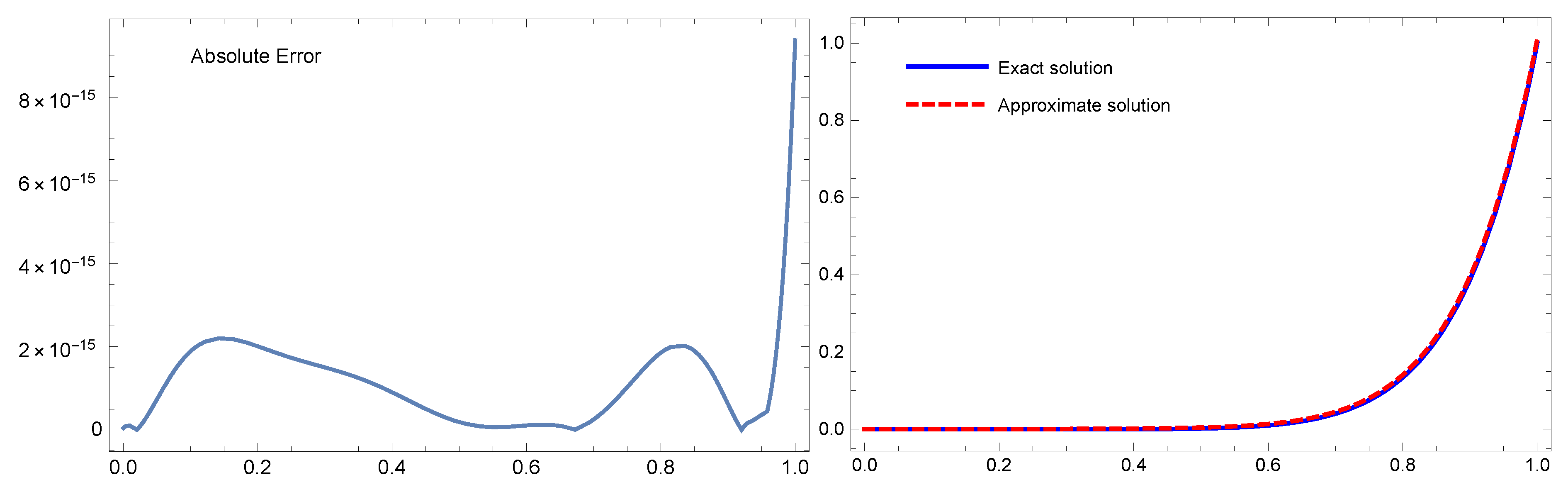
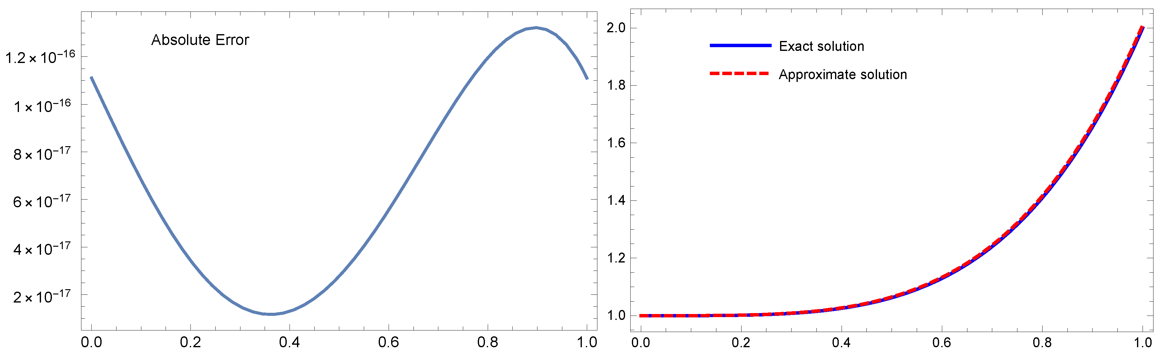
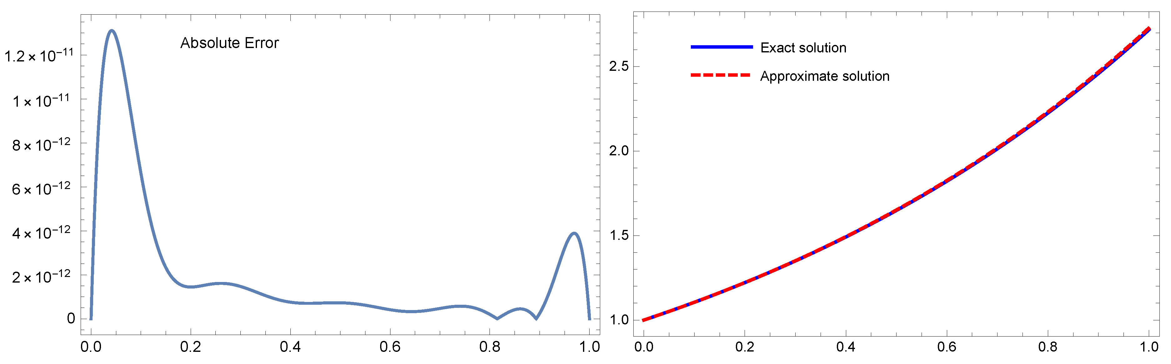
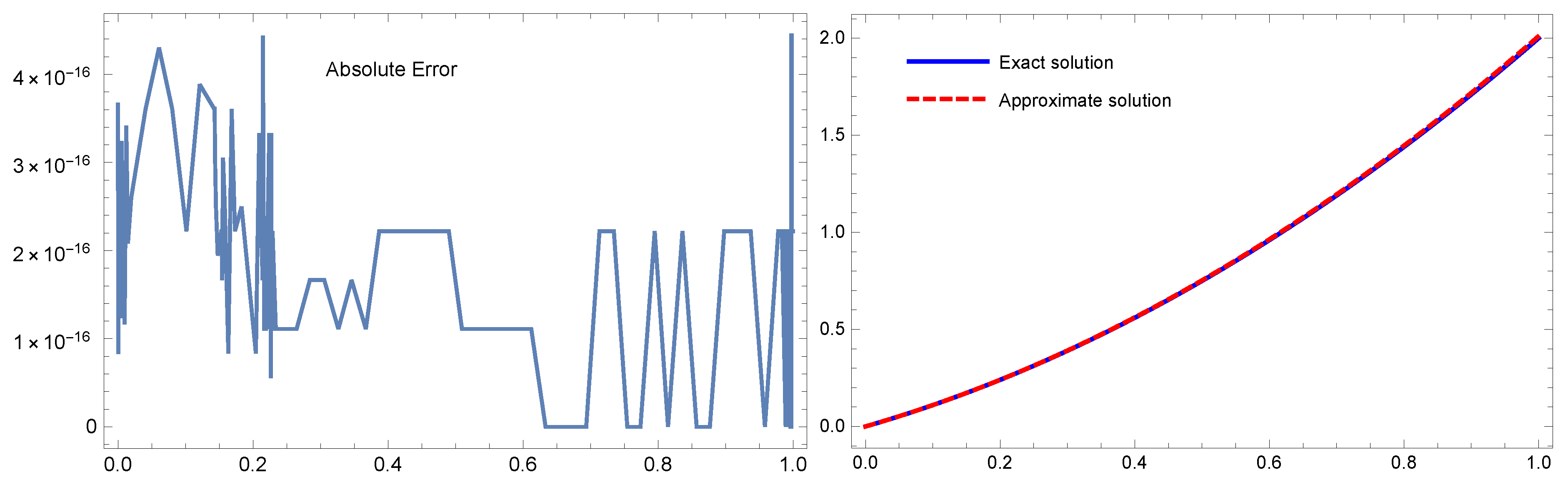
6. Numerical Applications

In this section, several examples are used to demonstrate the correctness and applicability of the methodology proposed in this article. Results acquired using the suggested method are compared to those obtained using other methods, revealing that the method put forward in this paper is appropriate and highly efficient. To demonstrate the accuracy of the proposed method, we calculated the following errors: the absolute error $\left(AE\right)$, $L_2$ error norm, and maximum absolute error $L_{\infty }$, respectively:

$$AE=|v\left(t_s\right)-v_n\left(t_s\right)|,s=0,1,2,\dots ,n,n\in {\mathbb{Z}}^{+},t_s\in ]0,\tau [.$$

(41)

$$L_2={\left({\int }_0^{\tau }{\left(v\left(t\right)-v_n\left(t\right)\right)}^{2}dt\right)}^{\frac{1}{2}},n\in {\mathbb{Z}}^{+},n\ge 2,t\in ]0,\tau [.$$

(42)

$$L_{\infty }=\underset{0\le s\le n}{\mathrm{Max}}\left\{\right|v\left(t_s\right)-v_n\left(t_s\right)\left|\right\},s=0,1,2,\dots ,n,n\in {\mathbb{Z}}^{+},t_s\in ]0,\tau [.$$

(43)

where $t,v\left(t\right)$ and $v_n\left(t\right)$ are the space vector, exact, and numerical solutions, respectively.

Remark 1. 

In all the following figures, the horizontal axis of the left figures refers to the parameter t and the vertical axis refers to the absolute error (AE) values. For the $right$ side of the figure, the horizontal line indicates the values of the parameter t, while the perpendicular refers to the exact $v\left(t\right)$ and approximate values $v_m\left(t\right)$ of the solutions.

Example 1 

([28,38]). Consider BNMFDE in the following formula:

$${\mathcal{D}}^{\frac{3}{2}}v\left(t\right)+{\mathcal{D}}^{\frac{1}{2}}v\left(t\right)+v^2\left(t\right)=t^{18}+\frac{2^{16}}{12155\sqrt{\pi }}{t}^{8.5}+\frac{2^{15}}{715\sqrt{\pi }}{t}^{7.5},t\in ]0,1[,$$

$$v\left(0\right)=0,v\left(1\right)=1.$$

The closed form solution to Example 1 is supplied by $v\left(t\right)=t^9$.

Table 1. $L_2$ and $L_{\infty }$ error comparison for Example 1 at distinct values of m.

m	${\mathit{L}}_2$-Error			${\mathit{L}}_{\mathit{\infty }}$-Error
	In [38]	In [28]	Our Method	In [38]	In [28]	Our Method
5	-	$2.8\times {10}^{-2}$	$7.1\times {10}^{-3}$	-	$1.7\times {10}^{-2}$	$1.1\times {10}^{-2}$
7	$7.3\times {10}^{-3}$	$5.9\times {10}^{-4}$	$3.0\times {10}^{-4}$	$8.2\times {10}^{-3}$	$2.9\times {10}^{-4}$	$5.0\times {10}^{-4}$
8	$5.4\times {10}^{-4}$	$3.5\times {10}^{-5}$	$1.7\times {10}^{-5}$	$1.2\times {10}^{-3}$	$1.8\times {10}^{-5}$	$2.1\times {10}^{-5}$
9	$4.1\times {10}^{-5}$	$3.2\times {10}^{-13}$	$1.5\times {10}^{-15}$	$7.0\times {10}^{-5}$	$2.2\times {10}^{-13}$	$9.4\times {10}^{-15}$

compares the error norms constructed using the proposed technique and the methods in [28,38] for various values of m.

Table 2. Absolute error (AE) when using the suggested methodology for Examples 1–3.

t	Example 1$,(\mathit{m}=9)$	Example 2$,(\mathit{m}=4)$	Example 3$,(\mathit{m}=9)$
0.1	$1.8871\times {10}^{-15}$	$6.8257\times {10}^{-17}$	$6.6140\times {10}^{-12}$
0.2	$2.0108\times {10}^{-15}$	$3.4284\times {10}^{-17}$	$1.4446\times {10}^{-12}$
0.3	$1.5017\times {10}^{-15}$	$1.4966\times {10}^{-17}$	$1.4693\times {10}^{-12}$
0.4	$9.0365\times {10}^{-16}$	$1.2967\times {10}^{-17}$	$7.5473\times {10}^{-13}$
0.5	$1.8475\times {10}^{-16}$	$2.7756\times {10}^{-17}$	$7.2764\times {10}^{-13}$
0.6	$1.0621\times {10}^{-16}$	$5.5600\times {10}^{-17}$	$4.1212\times {10}^{-13}$
0.7	$2.4807\times {10}^{-16}$	$8.9573\times {10}^{-17}$	$4.6985\times {10}^{-13}$
0.8	$1.8550\times {10}^{-15}$	$1.1955\times {10}^{-16}$	$1.9984\times {10}^{-13}$
0.9	$6.1943\times {10}^{-16}$	$1.3221\times {10}^{-16}$	$2.4409\times {10}^{-13}$

(second column) displays the absolute error results for Example 1 at $m=9$. In Figure 1, the absolute error is plotted at $m=9$; the analytical solutions is plotted on the left, and the numerical solutions are plotted on the right. From these results, it is obvious that the method in this paper produces results that are superior to those found in [28,38]. The numerical solution obtained with the proposed method is almost identical to the analytical solution.

Example 2 

([28,38]). Consider the following BNMFDE:

$$t{\mathcal{D}}^{\frac{5}{4}}v\left(t\right)+(1+2t^2)v\left(t\right){\mathcal{D}}^{\frac{1}{3}}v\left(t\right)=\frac{\Gamma \left(5\right)}{\Gamma \left(\frac{15}{4}\right)}{t}^{\frac{15}{4}}+\frac{\Gamma \left(5\right)}{\Gamma \left(\frac{14}{3}\right)}(1+2t^2)(1+t^4)t^{\frac{11}{3}},t\in [0,1],$$

$$v\left(0\right)=1,v\left(1\right)=2.$$

The analytical solution Example 2 is $v\left(t\right)=1+t^4$.

For a range of m values,

Table 3. Comparisons of the $L_2$ and $L_{\infty }$ errors for Example 2 at different values of m.

m	${\mathit{L}}_2$-Error			${\mathit{L}}_{\mathit{\infty }}$-Error
	In [38]	In [28]	Our Method	In [38]	In [28]	Our Method
2	$3.3\times {10}^{-1}$	$6.8\times {10}^{-1}$	$1.2\times {10}^{-1}$	$4.7\times {10}^{-1}$	$2.8\times {10}^{-1}$	$4.2\times {10}^{-1}$
4	$6.3\times {10}^{-2}$	$4.6\times {10}^{-9}$	$7.9\times {10}^{-17}$	$8.7\times {10}^{-2}$	$1.7\times {10}^{-9}$	$1.3\times {10}^{-16}$
8	$1.7\times {10}^{-6}$	$2.9\times {10}^{-9}$	$4.7\times {10}^{-16}$	$3.4\times {10}^{-6}$	$1.3\times {10}^{-9}$	$5.7\times {10}^{-16}$
10	$1.8\times {10}^{-8}$	$2.1\times {10}^{-9}$	$2.5\times {10}^{-15}$	$9.5\times {10}^{-8}$	$1.1\times {10}^{-9}$	$3.3\times {10}^{-15}$

compares the error norms produced by the suggested technique to the methods in [28,38]. The absolute error findings for Example 2 for $m=4$ are shown in Table 2 (column three). When $m=4$, Figure 2 depicts the absolute error on the left, with the analytical and numerical solutions shown on the right. These findings make it clear that the suggested approach yields outcomes that are better than those reported in [28,38]. Moreover, the approximate solution and the exact solution are very similar.

Example 3 

([28]). Consider the following nonlinear boundary fractional differential equation:

$${\mathcal{D}}^{\frac{1}{2}}v\left(t\right)+{\mathcal{D}}^{\frac{1}{3}}v\left(t\right)+v^2\left(t\right)=e^{2t}+E_{3/2}{t}^{0.5}+E_{5/3}{t}^{\frac{2}{3}},u\left(0\right)=1,t\in ]0,1[,$$

It is important to mention that $E_{3/2}$ and $E_{5/3}$ are the Mittag–Leffler functions. The exact solution for Example 3 is supplied by $v\left(t\right)=e^t$.

Table 4. $L_2$ and $L_{\infty }$ error comparisons for Example 3 with various m values.

m	${\mathit{L}}_2$-Error		${\mathit{L}}_{\mathit{\infty }}$-Error
	In [28]	Our Method	In [28]	Our Method
3	$7.0053\times {10}^{-3}$	$6.3008\times {10}^{-4}$	$1.1618\times {10}^{-3}$	$1.2280\times {10}^{-3}$
5	$1.4024\times {10}^{-5}$	$1.6760\times {10}^{-6}$	$2.3000\times {10}^{-6}$	$4.4244\times {10}^{-7}$
7	$1.6280\times {10}^{-8}$	$3.6500\times {10}^{-9}$	$2.6664\times {10}^{-9}$	$9.4535\times {10}^{-10}$
9	$3.6092\times {10}^{-10}$	$3.6500\times {10}^{-10}$	$9.6495\times {10}^{-11}$	$1.3108\times {10}^{-11}$

lists the error norms generated by the proposed methodology in comparison to the technique described by Dickson’s second-kind polynomials in [28] for a variety of m values. Table 2 displays the absolute error estimates for Example 3 for $m=9$ (the fourth column). The analytical and approximation solutions (right) are plotted in Figure 3 along with the absolute error (left) for Example 3 with $m=9$. These results demonstrate that the suggested strategy produces results that are superior to those mentioned in [28]. Furthermore, the actual solution and the approximation appear almost equivalent.

Example 4 

([29]). Consider the INMFDE of the Lane–Emden type problem:

$${\mathcal{D}}^{\mu }v\left(t\right)+\frac{1}{x^{\mu -{\mu }_1}}{\mathcal{D}}^{{\mu }_1}v\left(t\right)+e^{v\left(t\right)}=g\left(t\right),t\in ]0,1],v\left(0\right)=v^{\prime }\left(0\right)=0,$$

(44)

where

$$g\left(t\right)=2t^{2-\mu }\left(\frac{\Gamma (3-{\mu }_1)+\Gamma (3-\mu )}{\Gamma (3-{\mu }_1)\Gamma (3-\mu )}\right)+\frac{t^{1-\mu }}{\Gamma (2-{\mu }_1)}+e^{t^2+t}.$$

(45)

The analytical solution of Equation (44) when $\mu =1.5,{\mu }_1=0.5\mu$ is provided by $v\left(t\right)=t^2+t$.

Table 5. Comparison of AE for Example 4 with $\mu =1.5,{\mu }_1=0.5\mu$.

t	In [29] $(\mathit{N}=6)$	Proposed Method $(\mathit{m}=2)$
0.1	$1.02487\times {10}^{-13}$	$2.63678\times {10}^{-16}$
0.2	$9.95315\times {10}^{-14}$	$1.66533\times {10}^{-16}$
0.3	$9.57012\times {10}^{-14}$	$2.22045\times {10}^{-16}$
0.4	$9.09273\times {10}^{-14}$	$2.22045\times {10}^{-16}$
0.5	$8.48210\times {10}^{-14}$	$1.11022\times {10}^{-16}$
0.6	$7.72715\times {10}^{-14}$	$1.11022\times {10}^{-16}$
0.7	$6.88338\times {10}^{-14}$	0.0
0.8	$5.86198\times {10}^{-14}$	0.0
0.9	$4.66294\times {10}^{-14}$	0.0
1.0	$3.37508\times {10}^{-14}$	0.0

shows a comparison between the absolute error results produced by the suggested approach with $m=2$ and the method provided by the orthonormal Bernoulli’s polynomials in [29] with $m=6$ for Example 4. For Example 4 with $m=2$, Figure 4 plots the exact and numerical solutions on the right and the absolute error on the left. These results show that the recommended approach yields outcomes that are better than those reported in [29]. The analytical solution and the approximation appear to be nearly identical. Furthermore, the CPU time for the proposed method is lower $(m=2)$ and the results are better.

Example 5 

([30,39]). Finally, we turn our attention to another form of INMFDE known as the fractional-order Bratu differential equation type:

$${\mathcal{D}}^{\mu }v\left(t\right)-e^{2v\left(t\right)}=0,t\in ]0,1],\mu \in (1,2],v\left(0\right)=v^{\prime }\left(0\right)=0.$$

(46)

The exact answer that corresponds to Example 5 at $\mu =2$ is $v\left(t\right)=ln(sec(t\left)\right)$.

Table 6. AE reported for Example 5 according to [30,39] and our introduced technique.

t	In [30]	In [39]	Our Method $(\mathit{m}=5)$
$0.1$	$8.33\times {10}^{-6}$	$3.95\times {10}^{-6}$	$2.45\times {10}^{-15}$
$0.2$	$1.51\times {10}^{-7}$	$6.15\times {10}^{-6}$	$7.26\times {10}^{-15}$
$0.3$	$6.40\times {10}^{-7}$	$8.57\times {10}^{-6}$	$1.25\times {10}^{-14}$
$0.4$	$1.02\times {10}^{-6}$	$1.13\times {10}^{-5}$	$1.77\times {10}^{-14}$
$0.5$	$1.35\times {10}^{-6}$	$1.45\times {10}^{-5}$	$2.31\times {10}^{-14}$
$0.6$	$1.90\times {10}^{-6}$	$1.85\times {10}^{-5}$	$2.90\times {10}^{-14}$
$0.7$	$3.20\times {10}^{-6}$	$2.36\times {10}^{-5}$	$3.58\times {10}^{-14}$
$0.8$	$3.50\times {10}^{-6}$	$3.07\times {10}^{-5}$	$4.28\times {10}^{-14}$
$0.9$	$1.65\times {10}^{-6}$	$4.16\times {10}^{-5}$	$5.09\times {10}^{-14}$
$1.0$	$2.14\times {10}^{-5}$	$6.48\times {10}^{-6}$	$6.24\times {10}^{-14}$

reports the absolute error at $\mu =2$ generated by the recommended strategy with $m=5$ in comparison to the techniques published in [30,39] with $m=10$.

Table 7. Comparison of $L_{\infty }$ error for Example 5 using $\xi =2$ with various values of m in [39] and our proposed approach.

$\mathit{N}=\mathit{m}$ in [39]	${\mathit{L}}_{\mathit{\infty }}$-Error in [39]	Ours m	Our Method’s ${\mathit{L}}_{\mathit{\infty }}$-Error
5	$8.34\times {10}^{-4}$	3	$3.25\times {10}^{-9}$
10	$4.16\times {10}^{-5}$	5	$6.25\times {10}^{-14}$
20	$2.22\times {10}^{-6}$	7	$4.50\times {10}^{-16}$
40	$1.92\times {10}^{-7}$	8	$4.36\times {10}^{-16}$
80	$6.80\times {10}^{-9}$	10	$1.36\times {10}^{-16}$

displays the $L_{\infty }$ error results for Example 5 at various values of m for our suggested strategy and the technique in [39]. At $m=7$, Figure 5 plots the absolute error on the left, while the right-hand side of the figure shows the analytical and numerical solutions, respectively. Figure 6 describes the numerical solutions for Example 5 in the case of several values of the fractional-order parameter $\mu =2,1.9,1.8,1.7,1.5,1.3$ with $m=5$.

From the results of Table 6, it can be seen that better results are achieved with smaller terms, e.g., $m=5$. Table 7 provides accurate and sufficient results with small terms ($m=3,5,7,8,10$), while in [39] the authors used $m=5,10,20,40,80$. The figures show more accurate results and applicability for several fractional cases. The proposed method achieves significantly smaller absolute errors compared to those reported in previous works [30,39], and the numerical and analytical solutions are very similar. Overall, this comparison between the absolute errors reported in previous works and our proposed method clearly demonstrates the superiority of our approach in terms of accuracy and efficiency.

7. Conclusions

In this work, accurate numerical solutions for a class of nonlinear multi-term fractional differential equations have been proposed. Chebyshev’s third kind of polynomials are introduced as the basis of the solution. A general formulation for the Chebyshev third-kind operational matrices of integer and fractional-order derivatives is developed. Caputo fractional order derivatives have two main advantages: the first is that the derivative of the constant is zero, and the second is that the integer derivative of the initial and boundary conditions coincides with the derivative of classical forms. Because the Caputo fractional derivative enables the inclusion of conventional beginning and boundary conditions in the formulation of the issue, we have described fractional derivatives in the Caputo sense. In addition, we have discussed the error bound of the proposed approach. The multi-term problem is converted into a system of algebraic equations based on the proposed method, then solved numerically to obtain the unknown coefficients. The findings presented in the examples show how accurate these algorithms are. The comparisons carried out through numerical examples prove that our suggested methodology is more accurate and efficient than those in previously published works. Moreover, only a few shifted Chebyshev polynomials are required to produce an excellent outcome. Finally, it is important to note that the proposed methodology can be expanded to solve additional kinds of FDEs (partial or ordinary) appearing in a variety of applications.

References

1. Kilbas, A.A.; Srivastava, H.M.; Trujillo, J.J. Theory and Applications of Fractional Differential Equations; Elsevier: San Diego, CA, USA, 2006. [Google Scholar]
2. Podlubny, I. Fractional Differential Equations; Academic Press: New York, NY, USA, 1999. [Google Scholar]
3. Baleanu, D.; Balas, V.E.; Agarwal, P. Fractional Order Systems and Applications in Engineering; Elsevier: San Diego, CA, USA; Academic Press: New York, NY, USA, 2023. [Google Scholar]
4. Piotrowska, E.; Rogowski, K. Time-Domain analysis of fractional electrical circuit containing two ladder elements. Electronics 2021, 10, 475. [Google Scholar] [CrossRef]
5. Khazayinejad, M.; Nourazar, S.S. Space-fractional heat transfer analysis of hybrid nanofluid along a permeable plate considering inclined magnetic field. Sci. Rep. 2022, 12, 5220. [Google Scholar] [CrossRef]
6. Rabah, F.; Abukhaled, M.; Khuri, S.A. Solution of a complex nonlinear fractional biochemical reaction model. Math. Comput. Appl. 2022, 27, 45. [Google Scholar] [CrossRef]
7. Ionescu, C.; Lopes, A.; Copot, D.; Machado, J.A.T.; Bates, J.H.T. The role of fractional calculus in modeling biological phenomena: A review. Commun. Nonlinear Sci. Numer. Simul. 2017, 51, 141–159. [Google Scholar] [CrossRef]
8. Agarwal, P.; El-Sayed, A.A. Vieta-Lucas polynomials for solving a fractional-order mathematical physics model. Adv. Differ. Equ. 2020, 2020, 626. [Google Scholar] [CrossRef]
9. Arora, S.; Mathur, T.; Agarwal, S.; Tiwari, K.; Gupta, P. Applications of fractional calculus in computer vision: A survey. Neurocomputing 2022, 489, 407–428. [Google Scholar] [CrossRef]
10. Nagy, A.M.; El-Sayed, A.A. An accurate numerical technique for solving two-dimensional time fractional order diffusion equation. Int. J. Model Simul. 2019, 39, 214–221. [Google Scholar] [CrossRef]
11. El-Sayed, A.A.; Agarwal, P. Spectral treatment for the fractional-order wave equation using shifted Chebyshev orthogonal polynomials. J. Comput. Appl. Math. 2023, 424, 114933. [Google Scholar] [CrossRef]
12. Sweilam, N.H.; El-Sayed, A.A.; Boulaaras, S. Fractional-order advection-dispersion problem solution via the spectral collocation method and the non-standard finite difference technique. Chaos Solitons Fractals 2023, 144, 110736. [Google Scholar] [CrossRef]
13. Mokhtary, P.; Ghoreishi, F.; Srivastavac, H.M. The Müntz-Legendre Tau method for fractional differential equations. Math. Comput. Simul. 2022, 194, 210–235. [Google Scholar] [CrossRef]
14. Nedaiasl, K.; Dehbozorgi, R. Galerkin finite element method for nonlinear fractional differential equations. Numer. Algor. 2021, 88, 113–141. [Google Scholar] [CrossRef]
15. Youssri, Y.H.; Abd-Elhameed, W.M.; Ahmed, H.M. New fractional derivative expression of the shifted third-kind Chebyshev polynomials: Application to a type of nonlinear fractional Pantograph differential equations. J. Funct. Spaces 2022, 2022, 3966135. [Google Scholar] [CrossRef]
16. Arfan, M.; Khan, Z.A.; Zeb, A.; Shah, K. Study of numerical solution to some fractional order differential equation using Hermite polynomials. Int. J. Appl. Comput. Math. 2022, 8, 60. [Google Scholar] [CrossRef]
17. El-Sayed, A.A.; Boulaaras, S.; Sweilam, N.H. Numerical solution of the fractional-order logistic equation via the first-kind Dickson polynomials and spectral tau method. Math. Methods Appl. Sci. 2023, 46, 8004–8017. [Google Scholar] [CrossRef]
18. Agarwal, P.; El-Sayed, A.A.; Tariboong, J. Vieta-Fibonacci operational matrices for spectral solutions of variable-order fractional integro-differential equations. J. Comput. Appl. Math. 2021, 382, 113063. [Google Scholar] [CrossRef]
19. Ghafoori, S.; Motevalli, M.; Nejad, M.G.; Shakeri, F.; Ganji, D.D.; Jalaal, M. Efficiency of differential transformation method for nonlinear oscillation: Comparison with HPM and VIM. Curr. Appl. Phys. 2011, 11, 1567–1739. [Google Scholar] [CrossRef]
20. Baleanu, D.; Golmankhaneh, A.K.; Golmankhaneh, A.K.; Nigmatullin, R.R. Newtonian law with memory. Nonlinear Dyn. 2010, 60, 81–86. [Google Scholar] [CrossRef]
21. Hilfer, R. Application of Fractional Calculus in Physics; World Scientific: Singapore, 2000. [Google Scholar]
22. Hilfer, R. Mathematical and physical interpretations of fractional derivatives and integrals. In Handbook of Fractional Calculus with Applications, Volume1: Basic Theory; Kochubei, A., Luchko, Y., Eds.; De Gruyter: Berlin, Germany, 2019; pp. 47–85. [Google Scholar]
23. Han, W.; Chen, Y.M.; Liu, D.Y.; Li, X.L.; Boutat, D. Numerical solution for a class of multi-order fractional differential equations with error correction and convergence analysis. Adv. Differ. Equ. 2018, 2018, 253. [Google Scholar] [CrossRef]
24. Avci, I.; Mahmudov, N.I. Numerical solutions for multi-term fractional order differential equations with fractional Taylor operational matrix of fractional integration. Mathematics 2020, 8, 96. [Google Scholar] [CrossRef]
25. Doha, E.H.; Bhrawy, A.H.; Ezz-Eldien, S.S. Efficient Chebyshev spectral methods for solving multi-term fractional orders differential equations. Appl. Math. Model. 2011, 35, 5662–5672. [Google Scholar] [CrossRef]
26. Youssri, Y.H.; Abd-Elhameed, W.M. pectral solutions for multi-term fractional initial value problems using a new fibonacci operational matrix of fractional integration. Progr. Fract. Differ. Appl. 2016, 2, 141–151. [Google Scholar] [CrossRef]
27. Abd-Elhameed, W.M.; Alsuyuti, M.M. Numerical treatment of multi-term fractional differential equations via new kind of generalized Chebyshev polynomials. Fractal Fract. 2023, 7, 74. [Google Scholar] [CrossRef]
28. Nagy, A.M. Numerical solutions for nonlinear multi-term fractional differential equations via Dickson operational matrix. Int. J. Comput. Math. 2022, 99, 1505–1515. [Google Scholar] [CrossRef]
29. Sahu, P.K.; Mallicki, B. Approximate solution of fractional order Lane-Emden type differential equation by orthonormal Bernoulli’s polynomials. Int. J. Appl. Comput. Math. 2019, 5, 89. [Google Scholar] [CrossRef]
30. Babolian, E.; Javadi, S.; Moradi, E. RKM for solving Bratu-type differential equations of fractional order. Math. Methods Appl. Sci. 2016, 39, 1548–1557. [Google Scholar] [CrossRef]
31. Ghomanjani, F.; Shateyi, S. Numerical solution for fractional Bratu’s initial value problem. Open Phys. 2017, 15, 1045–1048. [Google Scholar] [CrossRef]
32. Hilfer, R. Threefold introduction to fractional derivatives. In Anomalous Transport: Foundations and Applications; Klages, R., Radons, G., Sokolov, I., Eds.; Wiley-VCH: Weinheim, Germany, 2008; pp. 17–74. [Google Scholar]
33. Teodoro, G.S.; Machado, J.A.T. Capelas de Oliveira, E. A review of definitions of fractional derivatives and other operators. J. Comput. Phys. 2019, 388, 195–208. [Google Scholar] [CrossRef]
34. Wang, Q.; Shi, X.; He, J.H.; Li, Z.B. Fractal calculus and its application to explanation of biomechanism of polar bear hairs. Fractals 2018, 26, 1850086. [Google Scholar] [CrossRef]
35. Wang, K.J.; Xu, P. Generalized variational structure of the fractal modified KdV-Zakharov-Kuznetsov equation. Fractals 2023, 31, 2350084. [Google Scholar] [CrossRef]
36. Wang, K.J.; Xu, P.; Shi, F. Nonlinear dynamic behaviors of the fractional (3+1)- dimensional modified Zakharov-Kuznetsov equation. Fractals 2023, 31, 2350088. [Google Scholar] [CrossRef]
37. Srivastava, H.M.; Adel, W.; Izadi, M.; El-Sayed, A.A. Solving Some Physics Problems Involving Fractional-Order Differential Equations with the Morgan-Voyce Polynomials. Fractal Fract. 2023, 7, 301. [Google Scholar] [CrossRef]
38. Pakchin, S.I.; Lakestani, M.; Kheiri, H. Numerical approach for solving a class of nonlinear fractional differential equation. Bull. Iranian Math. Soc. 2016, 42, 1107–1126. [Google Scholar]
39. Gharechahi, R.; Arabameri, M.; Bisheh-Niasar, M. Numerical solution of fractional Bratu’s initial value problem using compact finite difference scheme. Progr. Fract. Differ. Appl. 2021, 7, 103–115. [Google Scholar]
40. Alsuyuti, M.M.; Doha, E.H.; Ezz-Eldien, S.S. Galerkin operational approach for multi-dimensions fractional differential equations. Commun. Nonlinear Sci. Numer. Simul. 2022, 114, 106608. [Google Scholar] [CrossRef]
41. El-Sayed, A.A.; Agarwal, P. Numerical solution of multiterm variable-order fractional differential equations via shifted Legendre polynomials. Math. Meth. Appl. Sci. 2019, 41, 3978–3991. [Google Scholar] [CrossRef]
42. Duan, J.S.; Zhang, J.Y.; Qiu, X. Exact solutions of fractional order oscillation equation with two fractional derivative terms. J. Nonlinear Math. Phys. 2022, 30, 531–552. [Google Scholar] [CrossRef]
43. Heydari, M.H.; Avazzadeh, Z.; Haromi, M.F. A wavelet approach for solving multi-term variable-order time fractional diffusion wave equation. Appl. Math. Comput. 2019, 341, 215–228. [Google Scholar] [CrossRef]
44. Mustahsan, M.; Younas, H.M.; Iqbal, S.; Rathore, S.; Nisar, K.S.; Singh, J. An efficient analytical technique for time-fractional parabolic partial differential equations. Front. Phys. 2020, 8, 1–8. [Google Scholar] [CrossRef]
45. Kumar, S.; Gupta, V.; Gómez-Aguilar, J.F. An efficient operational matrix technique to solve the fractional order non-local boundary value problems. J. Math. Chem. 2022, 60, 1463–1479. [Google Scholar] [CrossRef]
46. Abd-Elhameed, W.M.; Badah, B.M.; Amin, A.K.; Alsuyuti, M.M. Spectral solutions of even-order BVPs based on new operational matrix of derivatives of generalized Jacobi polynomials. Symmetry 2023, 15, 345. [Google Scholar] [CrossRef]
47. Odibat, Z.M.; Shawagfeh, N.T. Generalized Taylor’s formula. Appl. Math. Comput. 2007, 186, 286–293. [Google Scholar] [CrossRef]
Figure 1. Example 1 with m = 9 ; the exact and an approximate solutions are shown on the right, while the absolute error is shown on the left.
Fractalfract 07 00784 g001
Figure 2. The absolute error (left) and the numerical and the analytical solutions (right) for Example 2 with m = 4 .
Fractalfract 07 00784 g002
Figure 3. For Example 3 with m = 9 , showing the absolute error (left) and the numerical and exact solutions (right).
Fractalfract 07 00784 g003
Figure 4. The the absolute error for Example 3 with m = 2 (left) and the approximate and exact solutions (right).
Fractalfract 07 00784 g004
Figure 5. The absolute error (left) and the close and numerical solutions for Example 5 (right) with m = 7 .
Fractalfract 07 00784 g005
Figure 6. The numerical and exact solutions for Example 5 with m = 5 for different values of the fractional parameter μ = 1.9 , 1.8 , 1.7 , 1.5 , 1.3 .
Fractalfract 07 00784 g006