Difference between Charge–Voltage Relations of Ordinary and Fractional Capacitors

Abstract

In an ordinary time-varying capacitor, there is debate on whether a time-domain multiplication or a time-domain convolution of capacitance and voltage determines charge. The objective of this work is to resolve this question by experiments on a time-varying capacitor in parallel with a resistor. It was implemented by a motor-driven potentiometer and op-amps. The response matched a power-law function over about two decades of time, and not an exponential, for several sets of parameters. This confirms the time-domain multiplication model. This result is the opposite of that obtained for a constant phase element (CPE) in its common time- and frequency-varying capacitor interpretation. This demonstrates that a CPE is fundamentally different from an ordinary time- and frequency-varying capacitor.

1. Introduction

In an ideal capacitor with capacitance C, the charge–voltage relationships in the time and frequency domains are:

$$q\left(t\right)=C·v\left(t\right)\iff Q\left(\omega \right)=C·V\left(\omega \right),$$

(1)

where lower-case letters denote the time domain, and capital letters denote the Fourier domain. The simple relation of (1) is no longer true when the capacitance varies with time as pointed out in [1]. In that case, the convolution operator is required, as a multiplication in one domain is equivalent to a convolution in the other. Convolution is defined by:

$$f\left(x\right)=g\left(x\right)\ast h\left(x\right)={\int }_{-\infty }^{\infty }g\left(\xi \right)h(x-\xi )\mathrm{d}\xi$$

(2)

In the time-varying capacitance case, only one of the following alternatives can be valid. The first one is:

$$q\left(t\right)=c\left(t\right)·v\left(t\right)\iff Q\left(\omega \right)=C\left(\omega \right)\ast V\left(\omega \right),$$

(3)

This time-domain multiplication is assumed in [2] and recommended in [3,4]. The alternative, based on time-domain convolution, is

$$q\left(t\right)=\tilde{c}\left(t\right)\ast v\left(t\right)\iff Q\left(\omega \right)=\tilde{C}\left(\omega \right)·V\left(\omega \right),$$

(4)

which is recommended in [1,5] based on the analysis of and measurements on systems with fractional capacitors, also called constant phase elements (CPEs). In this paper, fractional capacitors and constant phase elements are considered to be equivalent. Note that capacitance here has unit F/s, hence the terminology $\tilde{c}\left(t\right)$ and $\tilde{C}\left(\omega \right)$.

Here, we report the results from measurements on a time-varying non-fractional capacitor which lend support to the expression with time domain multiplication (3). We then show that ordinary and fractional capacitors follow different rules. This explains why different and seemingly conflicting results have been reported in the recent literature.

We first recall theory for time-varying capacitors and find the consequences of the two alternative models. We then analyze CPEs showing the charge–voltage response and the relationship with classical dielectric models, the Curie–von Schweidler current response, and the Kohlrausch charge response. Then, we discuss how an ordinary time-varying capacitor with enough range of variation can be built using op-amps and a motor-driven potentiometer. Finally, we report measurements that distinguish between the two alternatives.

2. Theory

The current–charge relation is by definition:

$$i\left(t\right)=\frac{\mathrm{d}}{\mathrm{d}t}q\left(t\right).$$

(5)

This means that there are also two alternative voltage–current relations corresponding to (3) and (4). The first one is:

$$i\left(t\right)=c\left(t\right)\frac{\mathrm{d}v\left(t\right)}{\mathrm{d}t}+\frac{\mathrm{d}c\left(t\right)}{\mathrm{d}t}v\left(t\right),$$

(6)

This equation is implemented in the Micro-Cap circuit simulator (ver. 12) from Spectrum Software while OrCAD PSpice (ver. 15.7) has implemented just the first term of (6). Simulink^® from The Mathworks, Inc. (Natick, MA, USA) gives the user a choice between the first term alone or both (Introduced in ver. R2008a).

The alternative is

$$i\left(t\right)=\frac{\mathrm{d}}{\mathrm{d}t}\left[\tilde{c}\left(t\right)\ast v\left(t\right)\right].$$

(7)

2.1. Temporal Responses of Linearly Increasing Capacitance

The capacitor is assumed to increase linearly with time

$$C\left(t\right)=C_0+\theta t.$$

(8)

As is the case in time-varying systems, the time variable in (8) denotes when the system starts changing. It is, in general, independent of the time of application of an excitation [6]. However, when the input is an impulse or a step, the two are usually the same, and this is assumed here.

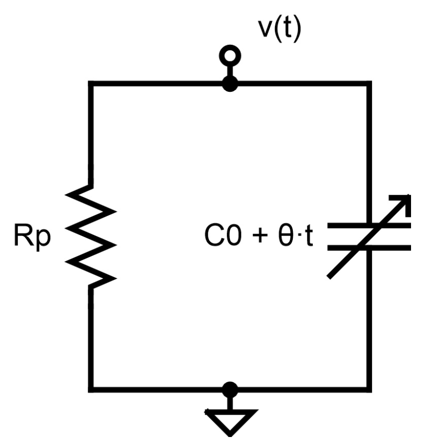
The capacitor is connected in parallel with a resistor $R_p$ as shown in Figure 1. In the following, we find two solutions that in the end are similar. The first is the particular (forced or transient) solution resulting from an input current impulse, which is such that the voltage response starts at $v\left(0\right)=V_0$. The second is the homogeneous (unforced or stationary) solution resulting from an initial voltage condition $v\left(0\right)=V_0$. The latter case is what we will measure later.

It is first assumed that the multiplication relation of (6) is valid. In that case, both the forced and the unforced voltage responses of the circuit of Figure 1 are:

$$v\left(t\right)=V_0{\left(1+\frac{t}{\tau }\right)}^{-\beta -1},\tau =\frac{C_0}{\theta },\beta =\frac{1}{R_p\theta },t>0.$$

(9)

The derivation is quite involved and is given in [2], which builds on the Appendix of [6]. In the limit as $t\gg \tau$, this is a power-law function where the voltage follows

$$v\left(t\right)\approx V_0{(t/\tau )}^{-\beta -1}.$$

(10)

As mentioned, a simplified version of the multiplication relation is assumed in some circuit simulation tools, where only the first term in (6) is included [2]. This model will also give a power-law result, but it will vary as ${(t/\tau )}^{-\beta }$. Thus, it is easy to distinguish from (10).

The second follows an analysis of the response if the convolution relation of (7) is assumed. First, it has to be realized that the time-varying capacitance expression in (8) is in the frequency domain. Therefore, a constant capacitor, $C\left(\omega \right)=C_0$, corresponds to $C_0\delta \left(t\right)$ in the time domain, with unit F/s. Likewise, a linearly increasing capacitor is the integral of a constant capacitor, and the integral of the delta function $\delta \left(t\right)$ is the step function $u\left(t\right)$, giving

$$\tilde{c}\left(t\right)=C_0\delta \left(t\right)+\theta u\left(t\right).$$

(11)

It may be noted that this result is the temporal derivative of (8) when an implicit step function is assumed in (8), i.e., $\tilde{c}\left(t\right)=\mathrm{d}C\left(t\right)/\mathrm{d}t$. This is an alternative explanation for why the additional differentiation appears in Equation (9) of [7]; see the discussion in [3,8].

Inserted in (7), the current is:

$$\begin{array}{cc}\hfill i\left(t\right)& =\frac{\mathrm{d}}{\mathrm{d}t}\left[C_0\delta \left(t\right)\ast v\left(t\right)+\theta u\left(t\right)\ast v\left(t\right)\right]+v\left(t\right)/R_p\hfill \\ \hfill & =\frac{\mathrm{d}}{\mathrm{d}t}\left[C_{0}v\left(t\right)+\theta \int v\left(t\right)\mathrm{d}t\right]+v\left(t\right)/R_p\hfill \\ \hfill & =C_0\frac{\mathrm{d}v\left(t\right)}{\mathrm{d}t}+\left(\theta +1/R_p\right)v\left(t\right).\hfill \end{array}$$

(12)

The voltage response to a current impulse is found by setting the above expression to 0, and this gives a differential equation with solution

$$v\left(t\right)=V_0{\mathrm{e}}^{-t/{\tau }^{\prime }},{\tau }^{\prime }=\frac{C_0}{\theta +1/R_p},$$

(13)

where $V_0$ is an initial value determined by the amplitude and duration of the input current impulse.

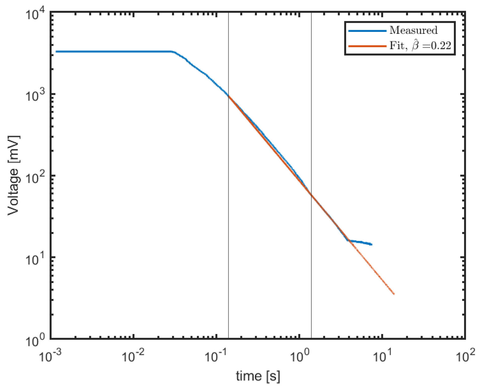
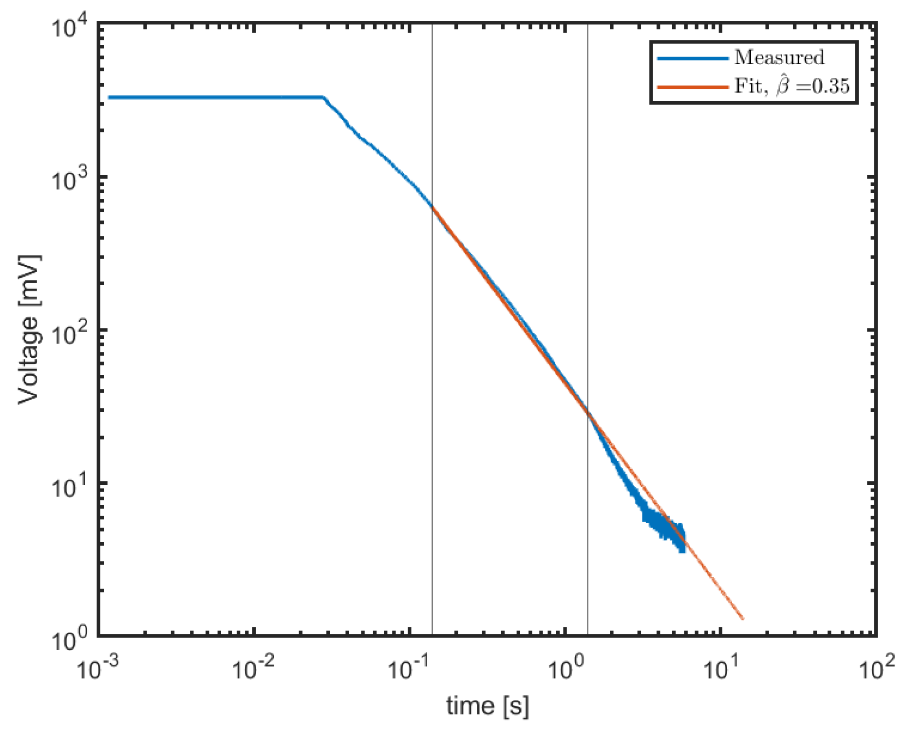
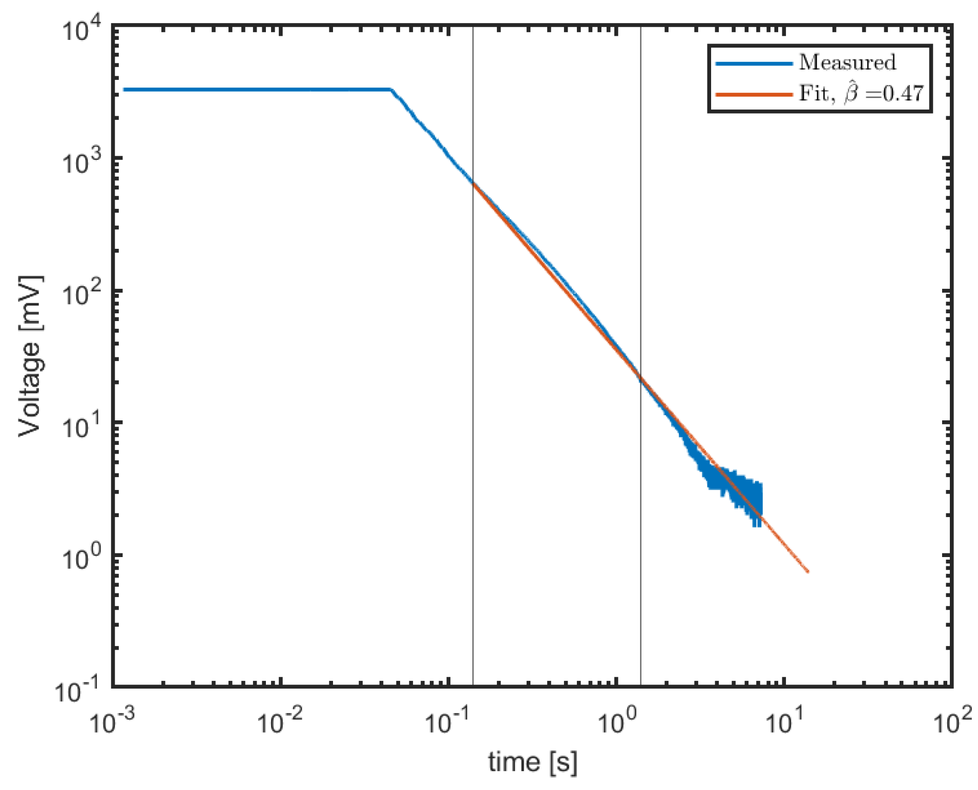
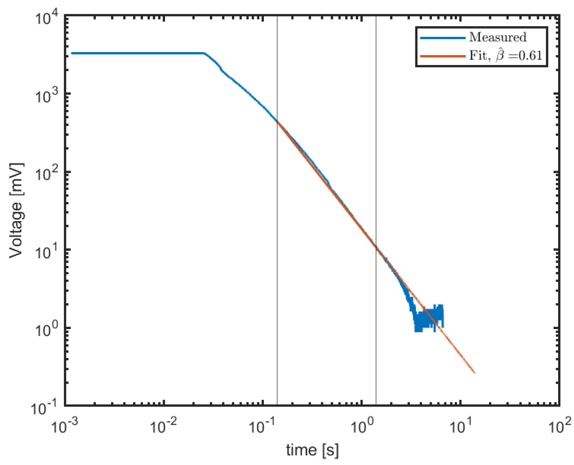
Thus, in order to distinguish whether (6) or (7) is valid for a time-varying capacitor, one needs to find the voltage response to a current impulse or an initial voltage and check whether it follows the power-law response of (10) or the exponential response of (13). If it follows a power law, it should be checked whether the exponent is $-\beta -1$ or just $-\beta$.

2.2. Constant Phase Element

The constant phase element (CPE) is a circuit element with a history going back to Cole [9,10]. It is defined by the impedance in the frequency domain [11]:

$$Z\left(\omega \right)=\frac{V\left(\omega \right)}{I\left(\omega \right)}=\frac{1}{{\left(\mathrm{j}\omega \right)}^{\alpha }{C}_{\alpha }},0<\alpha \le 1.$$

(14)

The equivalent capacitance is:

$$\tilde{C}\left(\omega \right)={\left(\mathrm{j}\omega \right)}^{\alpha -1}{C}_{\alpha }.$$

(15)

As the order $\alpha$ approaches unity, it becomes an ordinary capacitor, and for $\alpha =0$ it simplifies to an ordinary resistor. Inverse Fourier transformation of (15) gives:

$$\tilde{c}\left(t\right)=\frac{C_{\alpha }}{\mathrm{\Gamma }(1-\alpha )}{t}^{-\alpha }$$

(16)

As noted, a tilde is used for $\tilde{C}\left(\omega \right)$ and $\tilde{c}\left(t\right)$, as these are not capacitances in the ordinary sense. The equivalent capacitance of a CPE should therefore be found in some other way, e.g., by finding the capacitance which gives the same time constant as the CPE in an RC-circuit [12].

2.2.1. Charge–Voltage Relation for CPE

In the time domain, the current–voltage relation of the CPE is given by a fractional derivative:

$$i\left(t\right)=C_{\alpha }\frac{{\mathrm{d}}^{\alpha }v\left(t\right)}{\mathrm{d}{t}^{\alpha }}.$$

(17)

When (5) is combined with (17), the result is

$$\frac{{\mathrm{d}}^{1-\alpha }}{\mathrm{d}{t}^{1-\alpha }}q\left(t\right)=C_{\alpha }v\left(t\right).$$

(18)

This is a result from [4], where it is also shown that in the case of a time-varying CPE, the relation is

$$\frac{{\mathrm{d}}^{1-\alpha }}{\mathrm{d}{t}^{1-\alpha }}q\left(t\right)=C_{\alpha }\left(t\right)v\left(t\right).$$

(19)

On the one hand, for the special case $\alpha =1$, where the model becomes an ordinary capacitor, (19) will simplify to (6), and (18) to the time-domain multiplication of (3).

On the other hand, when (18) is solved for the charge, the result is:

$$q\left(t\right)=C_{\alpha }\frac{{\mathrm{d}}^{\alpha -1}}{\mathrm{d}{t}^{\alpha -1}}v\left(t\right)=\tilde{c}\left(t\right)\ast v\left(t\right).$$

(20)

This is the convolution description of (4), and the result is a consequence of the frequency domain definition of the CPE in (14).

With the ordinary time-varying capacitor, there may be uncertainty as to which of the charge–voltage responses are valid as shown in the previous section. Therefore, experimental evidence, as in the remainder of this paper, is needed to decide between the two models. This is different for the CPE, as the charge–voltage response is given by a convolution in time due to the way it has been defined in (14).

2.2.2. Temporal Response of CPE

Due to the singularity as the frequency approaches zero, it is evident that the CPE is an idealized circuit element. As capacitance is $C={\epsilon }_0{\epsilon }_{r}A/d$, where A is the plate area, d is the plate distance, and ${\epsilon }_0$ is the permittivity of vacuum, the CPE also corresponds to a singular model for relative permittivity:

$${\epsilon }_r\left(\omega \right)=\frac{{\epsilon }_s}{{\left(\mathrm{j}\omega {\tau }_c\right)}^{1-\alpha }},$$

(21)

where ${\tau }_c$ is a characteristic relaxation time, and ${\epsilon }_s=C_{\alpha }{\tau }_c^{1-\alpha }$.

It is not uncommon to inverse transform (21) and obtain the Curie–von Schweidler law found below; see [4,7,13]. But as this law also is singular, we find that it gives more insight to view both the CPE and the Curie–von Schweidler law as limiting cases of the response of well-behaved standard dielectric models [14].

The most general of these dielectric models, the Havriliak–Negami model, has a relative permittivity of

$${\epsilon }_r\left(\omega \right)={\epsilon }_{\infty }+\frac{{\epsilon }_s-{\epsilon }_{\infty }}{{\left(1+{\left(\mathrm{j}\omega {\tau }_c\right)}^{{\gamma }_1}\right)}^{{\gamma }_2}},$$

(22)

where $0<{\gamma }_1,{\gamma }_2\le 1$ are parameters that characterize the model. Assuming ${\epsilon }_{\infty }=0$, $\omega {\tau }_c\gg 1$, and ${\gamma }_1·{\gamma }_2=1-\alpha$ will lead to (21). Therefore, the CPE can be found in the limit from either the Havriliak–Negami model, the Cole–Davidson model (${\gamma }_1=1$), or the Cole–Cole model (${\gamma }_2=1$).

Here, the latter case is analyzed. In [14], it is shown that the time-domain current step response is proportional to the response function $\varphi \left(t\right)$ of [15]. The response function is the inverse Fourier transform of the relative permittivity in normalized form, ${\epsilon }^{\prime }\left(\omega \right)=\left({\epsilon }_r\left(\omega \right)-{\epsilon }_{\infty }\right)/\left({\epsilon }_s-{\epsilon }_{\infty }\right)$. Taking into account that $\alpha$ in [14] is $1-\alpha$ here, the Cole–Cole model gives:

$$\begin{array}{cc}\hfill \varphi \left(t\right)& =\frac{1}{{\tau }_c}{\left(\frac{t}{{\tau }_c}\right)}^{-\alpha }{\mathrm{E}}_{1-\alpha ,1-\alpha }\left(-{\left(\frac{t}{{\tau }_c}\right)}^{1-\alpha }\right)\hfill \\ \hfill & \sim \left\{\begin{array}{cc}\frac{1}{{\tau }_c\mathrm{\Gamma }(1-\alpha )}{\left(\frac{t}{{\tau }_c}\right)}^{-\alpha }\hfill & ,t\ll {\tau }_c\hfill \\ \frac{1}{{\tau }_c\mathrm{\Gamma }(\alpha -1)}{\left(\frac{t}{{\tau }_c}\right)}^{\alpha -2}\hfill & ,t\gg {\tau }_c,\hfill \end{array}\right.\hfill \end{array}$$

(23)

where ${\mathrm{E}}_{\alpha ,\beta }$ is the two-parameter Mittag–Leffler function. The small time approximation is the Curie–von Schweidler law from 1889/1907.

Likewise, in [14] it is shown that the charge step response is proportional to the relaxation function, $\mathrm{\Psi }\left(t\right)$, of [15]. The relaxation function is the inverse Fourier transform of $\left(1-{\epsilon }^{\prime }\left(\omega \right)\right)/\mathrm{j}\omega$ and is for the Cole–Cole model:

$$\begin{array}{cc}\hfill \mathrm{\Psi }\left(t\right)& ={\mathrm{E}}_{1-\alpha ,1}\left(-{\left(\frac{t}{{\tau }_c}\right)}^{1-\alpha }\right)\hfill \\ \hfill & \sim \left\{\begin{array}{cc}exp\left[\frac{-{(t/{\tau }_c)}^{1-\alpha }}{\mathrm{\Gamma }(2-\alpha )}\right]\hfill & ,t\ll {\tau }_c\hfill \\ \frac{1}{\mathrm{\Gamma }\left(\alpha \right)}{\left(\frac{t}{{\tau }_c}\right)}^{\alpha -1}\hfill & ,t\gg {\tau }_c.\hfill \end{array}\right.\hfill \end{array}$$

(24)

The small time approximation is a stretched exponential which corresponds to the Kohlrausch law [14] from 1854. This demonstrates the close relationship between the CPE, the standard dielectric models, and the classical current and charge responses.

2.2.3. Inductive CPE

An inductive CPE of order ${\alpha }^{\prime }$ is defined by the extension of the results for the capacitive CPE [2]:

$$Z\left(\omega \right)={\left(\mathrm{j}\omega \right)}^{{\alpha }^{\prime }}{L}_{{\alpha }^{\prime }},0<{\alpha }^{\prime }\le 1.$$

(25)

This can be considered to be a capacitive CPE, where $\alpha =-{\alpha }^{\prime }$ and it will have a similar temporal response as that of (23) with voltage and current-changing roles, i.e., voltage proportional to $t^{-{\alpha }^{\prime }-1}$ for small temporal arguments. The similarity with the temporal response of the linearly varying capacitance in (10) is striking, and indicates one way of making a circuit with the same voltage response as a CPE as noted in [2].

3. Method

The results reported here were found during an attempt to make a circuit with the same voltage response as the inductive CPE, exploiting the just-mentioned similarity in responses. In our first attempt at circuit realization, we used the circuit of Figure 2 of [16] consisting of two op-amps and a voltage-controlled resistor configured to yield a voltage-controlled capacitor. The voltage-controlled resistor was implemented by a JFET operating in the non-saturated or triode region. The circuit was not very successful due to the restricted range of variation of the JFET resistance that was possible to achieve.

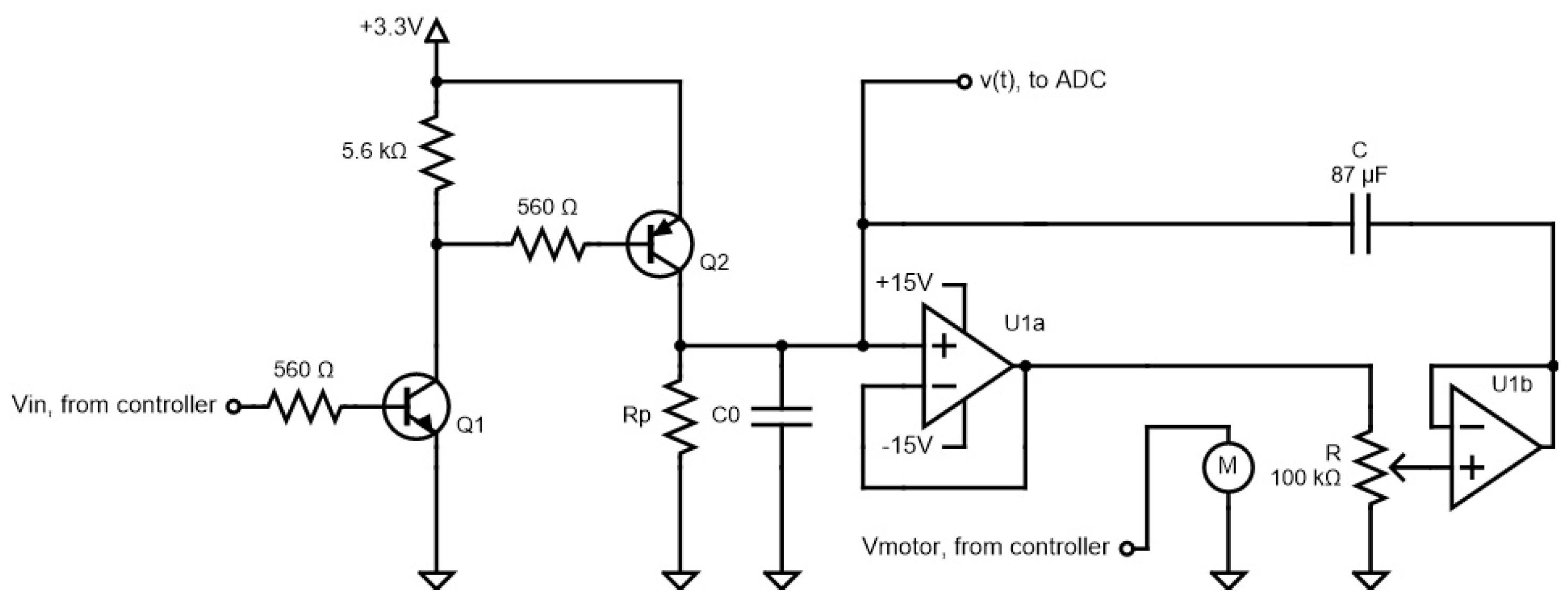
To improve performance, the JFET was substituted with a potentiometer mechanically coupled to a stepper motor using a 3D-printed adapter. The stepper motor was controlled by a microcontroller programmed in the Arduino programming environment. In this way, a precise time-varying resistor can be realized, but as it is a circuit with physically moving parts, it will be much slower than the JFET circuit. The circuit diagram is shown in Figure 2.

The components used were:

• Potentiometer: Bourns 91A1A-B28-B20, 240${}^{\circ }\pm 5^{\circ }$, 100 k$\mathrm{\Omega }$ $\pm 20\%$, 1 Watt, linear taper, measured to be $R=109 \mathrm{k}\mathrm{\Omega }$.
• Motor: 28BYJ-48, nominally 2048 steps per revolution.
• Microcontroller: Adafruit Metro M0 Express.

The capacitor was made by connecting eight ceramic capacitors with nominal value $10 \mathrm{\mu }\mathrm{F}$ in parallel. The total capacitance was measured with a component tester [17] to have a value of $C=87 \mathrm{\mu }\mathrm{F}$. Off-the-shelf capacitors may have a capacitance which varies with frequency, but this particular component tester measures the capacitance by means of the time constant for a discharge. As this is similar to how the capacitor is used in our circuit, the measured value is relevant for our circuit.

The purpose of $Q_1$ and $Q_2$ was to set the initial voltage $v\left(t\right)=V_0$ over $R_p$ and the time-varying capacitor. As the motor starts rotating the potentiometer, transistor $Q_2$ is opened so that the monitored voltage $v\left(t\right)$ is no longer fixed but is free to vary. The op-amps used are not very critical since the frequency is very low. The most important parameters are a high open-loop gain, a high input impedance, and a low output impedance. The LM358 dual op-amp was used, with satisfactory results.

The measurement of $v\left(t\right)$ was performed by using a 16-bit analog-to-digital converter (Adafruit ADS1115) connected to a separate microcontroller and sampling at 860 Hz.

First, the motor-driven potentiometer was connected to a DC source, and it was verified that it actually worked as a linearly varying resistor. The time $\Delta t$ from zero to max resistance was $\Delta t\approx 2.64 \mathrm{s}$. This gives the value for the rate of change of the resistance $\varphi$:

$$\varphi =\frac{\mathrm{d}R}{\mathrm{d}t}=\frac{109 \mathrm{k}\mathrm{\Omega }}{2.64 \mathrm{s}}\approx 41.3 \mathrm{k}\mathrm{\Omega }/\mathrm{s}.$$

(26)

The number of steps of the stepper motor used in practice is due to the limited rotation angle of the potentiometer $2048·{240}^{\circ }/{360}^{\circ }=1365$.

The time-varying capacitor as seen between the ground and the input of op-amp $U_1$, marked $v\left(t\right)$, is given by the value of the feedback capacitor C and the Miller effect. The negative voltage gain of the two unity gain amplifiers $U_1$ and $U_2$ and the potentiometer combined is:

$$A_v=-\frac{R-r\left(t\right)}{R},$$

(27)

where $r\left(t\right)$ is the resistor of the upper part of the potentiometer R. The input impedance as a function of the impedance of the feedback capacitor $Z_C$ is:

$$Z_{in}=\frac{Z_C}{1+A_v}=\frac{1}{\mathrm{j}\omega C}\frac{R}{r\left(t\right)}.$$

(28)

When the capacitor $C_0$ also is taken into account, the equivalent capacitance is:

$$C\left(t\right)=C_0+C\frac{r\left(t\right)}{R}=C_0+C\frac{\varphi t}{R}.$$

(29)

The coefficient of variation of the capacitor, $\theta$ of (8), therefore takes the value

$$\theta =\frac{\mathrm{d}C\left(t\right)}{\mathrm{d}t}=C\frac{\varphi }{R}=\frac{C}{\Delta t}\approx \frac{87 \mathrm{\mu }\mathrm{F}}{2.64 s}\approx 33 \mathrm{\mu }\mathrm{F}/\mathrm{s}.$$

(30)

The capacitor $C_0$ was not implemented by any physical capacitor. It represents mechanical effects in the motor–potentiometer system, and its value is estimated from the measurements.

4. Results and Discussion

Variable Capacitor Circuit

The results were obtained by measuring the voltage response to an initial input voltage for different values of the parallel resistor. The measurements are reported in Figure 3, Figure 4, Figure 5 and Figure 6. The time before the curves start falling represents the time constant, $\tau$, of (9). It is caused by the mechanical slack in the motor–potentiometer system and is in the range 25–$50 \mathrm{m}\mathrm{s}$. It can therefore safely be neglected compared to the measurement time of $2.64$ s, verifying that we can expect the simple power-law expression of (10) to be accurate (provided that (6) is correct). This range of values for $\tau$ corresponds to $C_0$ in the order of $1 \mathrm{\mu }\mathrm{F}$.

The expected $\beta$-values were calculated from (9) as

$$\beta =\frac{\Delta t}{R_{p}C}=\frac{2.64 \mathrm{s}}{R_p·87 \mathrm{\mu }\mathrm{F}},$$

(31)

and $R_p$ and the expected value for $\beta$ are shown in the first columns of

Table 1. Table of resistor values, $R_p$, expected value of $\beta$, and value of $\widehat{\beta }$ estimated from (32).

${\mathit{R}}_{\mathit{p}}$	$\mathsf{\beta }$	$\widehat{\mathsf{\beta }}$	Figure
150k	0.20	0.22	Figure 3
82k	0.37	0.35	Figure 4
68k	0.45	0.47	Figure 5
47k	0.65	0.61	Figure 6

.

Beyond a time of $\Delta t\approx 2.64$ s, the curves deviate from a power law, as the potentiometer stops moving, and the circuit behaves like a simple RC-circuit with an exponential fall-off.

The estimate of order is shown in these figures and in the third column of Table 1. The estimate was found by picking measured values over one decade in the range $\tau <t<\Delta t$. The vertical lines at $t_1=139.5$ ms and $t_2=10t_1$ show the values used. The estimate is:

$$\widehat{\beta }=-\frac{lnv\left(t_2\right)-lnv\left(t_1\right)}{ln{t}_2-ln{t}_1}-1.$$

(32)

As can be seen from the figures, the relaxation follows a power law for about two decades of time. This is adequate for concluding that the response is the power law of (10) and not the exponential decay of (13). Comparing columns 2 and 3 in Table 1, there is a difference in the order of 0.01–0.04, which indicates that there is also a good correlation between the theoretic $\beta$-value expected from the component values and the estimated value from the measured data.

5. Conclusions

The voltage response of the parallel combination of a resistor and a linearly increasing capacitor was measured to follow a power law over about two decades of time, and the exponent matched the expected value from the theoretical model. This is confirmation that the two-term time-domain multiplication definition of current in a capacitor of (6) is correct for this circuit. This is in contrast to the constant phase element, which when interpreted as a time- and frequency-varying capacitance, as is usually done, follows the time domain convolution of (7). This demonstrates that a CPE is a fundamentally different component from the time- and frequency-varying capacitance.