Article

A Fractional-Order Fidelity-Based Total Generalized Variation Model for Image Deblurring

School of Mathematics, Harbin Institute of Technology, Harbin 150001, China
*
Author to whom correspondence should be addressed.
Fractal Fract. 2023, 7(10), 756; https://doi.org/10.3390/fractalfract7100756
Submission received: 8 September 2023 / Revised: 4 October 2023 / Accepted: 12 October 2023 / Published: 13 October 2023

Abstract

:
Image deblurring is a fundamental image processing task, and research for efficient image deblurring methods is still a great challenge. Most of the currently existing methods are focused on TV-based models and regularization term construction; little efforts are paid to model proposal and correlated algorithms for the fidelity term in fractional-order derivative space. In this paper, we propose a novel fractional-order variational model for image deblurring, which can efficiently address three different blur kernels. The objective functional contains a fractional-order gradient fidelity term and a total generalized variation (TGV) regularization term, and it highlights the ability to preserve details and eliminate the staircase effect. To solve the problem efficiently, we provide two numerical algorithms based on the Chambolle-Pock primal-dual method (PD) and the alternating direction method of multipliers (ADMM). A series of experiments show that the proposed method achieves a good balance between detail preservation and deblurring compared with several existing advanced models.

1. Introduction

Image deblurring aims to get a clean, sharp image from a noisy, blurred image. Blurs can be observed in many fields such as out-of-focus blur in X-ray imaging because of the poor localization of the point spread function and motion blur caused by the movement of the person. Generally, the image blurring process can be modeled as the convolution of an original clear image with a shift-invariant blur kernel plus additive Gaussian white noise, i.e.,
f = K u + n ,
where u : Ω R 2 R is the original clean image, K is the convolution operator, and n is Gaussian noise with zero mean and variance σ 2 . According to whether the blur kernel K is prior knowledge, the problem of image deblurring can be divided into non-blind deblurring and blind deblurring. When K is known exactly, the problem is obtaining a clean image u from the observed image f and prior knowledge K; when K is unknown, the problem is estimating the blur kernel K first and then obtaining the clear image u from image f.
For the restoration of a blurred image, scientists take advantage of some prior knowledge of the unknown image u by adding a regularization term, which can be modeled as follows:
min u { Φ ( u ) + μ 2 K u f 2 2 } ,
where K u f 2 is called the fidelity term and Φ ( u ) is called the regularization term, and μ is a tuning parameter to balance the weight between the fidelity term and the regularization term. There are many methods that have been proposed for image restoration. Blind deconvolution image restoration [1,2] performs image restoration based on degradation models and prior knowledge, so it can adapt to different types and degrees of image degradation. However, blind deconvolution image restoration usually requires complex models and algorithms to model and process the degradation process of images, which makes it difficult to apply in practice. In addition, the unsuitability of inverse problems makes blind deconvolution image restoration unable to guarantee the uniqueness of solutions. The PSF restoration method [3,4] aims to reduce blur and noise in the image by calculating and estimating PSF, thus restoring the sharpness and detail of the image. However, it is sensitive to noise in the image, which may be amplified and affect the quality of the restored image. An image recursive filter [5,6] is an effective image smoothing and denoising filter, which calculates the value of the output pixel by the weighted average of the current pixel and its neighbors. However, the design and optimization of the image recursive filter is relatively complex, and there is a poor effect of noise suppression, which is easily introduces artifacts or distortion. In the field of variation image restoration, the most famous model in image restoration is the TV model, which is as follows:
min u B V ( Ω ) Ω | D u | + μ 2 K u f 2 2 .
Actually, TV was originally proposed in [7] for image denoising, and then it was extended to image deblurring in [8]. The TV model is a popular method that can effectively reduce the noise and blur in the image, and also preserve the sharp edge and texture detail of the image. However, TV regularization tends to get a piecewise constant solution, and, therefore, it easily causes a staircase effect. In order to efficiently suppress the staircase artifacts, numerous models with improved regularization terms have been proposed. This includes high-order partial differential equations [9] and higher-order TV methods (HOTV) [10], total variation regularization methods [11,12], sparsity regularization models [13,14], and fractional-order TV (FOTV) models [15,16]. In addition, nonlocal total variation (NLTV) [17,18] and block-matching 3-D (BM3D) [19,20] have been the most promising deblurring methods for recovering texture. Although NLTV and BM3D have shown good performance in image restoration, the NLTV functional minimization problem has always been a difficult optimization problem because of its high computation complexity and the non-differentiability, and the BM3D method has limited effectiveness in processing high-noise images and motion-blurred images.
Another method to overcome the staircase effect is the total generalized variation (TGV) regularization, which was firstly proposed by Bredies et al. as a penalty function in [21]. As an extension of TV regularization, TGV has good properties such as rotational invariance, lower semi-continuity, and convexity. The results show that the TGV regularization method can preserve the details of image edges and textures and suppress the staircase effect. In addition, the scalar weight α = ( α 1 , α 0 ) of the second-order TGV regularization model has multiple parameters, and better image restoration results can be achieved by adjusting the parameters, so the TGV model has been extensively studied in image restoration [22,23,24,25] and medical imaging [26]. It can be formulated as:
min u { TGV α 2 ( u ) + 1 2 λ K u f 2 2 } .
Although the TGV regularization model has many advantages, it tends to amplify the noise while restoring the image detail, creating artifacts or distortions, and due to the sensitivity of parameters, it may lead to poor deblurring results or excessive smoothing results (see [27,28]).
In this paper, aiming at achieving a good performance for image restoration, we propose a fractional-order fidelity-based total generalized variation model (FTGV) for image deblurring. The objective function takes the TGV as the regularization term that can suppress staircase effect, preserve edges and a fractional-order gradient fidelity term to preserve more details, and get a trade-off between edge preservation and blur removal by adjusting the regularization parameters. Then, based on the non-smoothing of the regularization term of the variation model and the non-convexity of the fractional fidelity term, we propose two optimization algorithms based on the primal-dual (PD) and alternating direction multiplier (ADMM), which transform the fractional problem into subproblems with less computation by introducing auxiliary variables, and finally solve the minimization problem by alternate iteration strategy. By precisely adjusting step size parameters and penalty parameters, the two algorithms are insensitive to the weights α = ( α 1 , α 0 ) , non-integer order γ , and balance parameters β in the variational model, and run faster, thus making the model more robust and efficient.
The rest of this paper is organized as follows. In Section 2, we present a brief introduction of TGV model, and then give the new deblurring model and the discrete form for objection functional. We provide the numerical scheme based on the PD algorithm and ADMM algorithm to solve the proposed model and analyze the convergence in Section 3. Numerical experiments are shown to illustrate the performance of the proposed model in Section 4.

2. Proposed Model

In this section, we first review the classic total generalized variation method (TGV) and some notations. Afterwards, we give the new model for image deblurring and its discrete form.

2.1. Review of TGV

The concept of total generalized variation (TGV) was proposed by Bredies et al. in [21]. The TGV of order k with positive weights α = ( α 0 , α 1 , , α k 1 ) is defined as:
TGV α k ( u ) = sup { Ω u div k v d x | v C c k ( Ω , Sym k ( R d ) ) , div j v α j , j = 0 , , k 1 } ,
where C c k ( Ω , Sym k ( R d ) ) denotes the space of the compactly supported symmetric tensor field and Sym k ( R d ) is the space of symmetric tensors on R d , which has the form:
Sym k ( R d ) = { ξ : R d × × R d R | ξ is multilinear and symmetric } .
When k = 1 , Sym 1 ( R d ) = R d , TGV 1 1 ( u ) = TV ( u ) , thus it is clear that TGV is a generalization of TV, when k = 2 , Sym 2 ( R d ) ) denotes the space of all symmetric S d × d matrices. Particularly, we take the second-order TGV [29] in the proposed model, it has form:
TGV α 2 ( u ) = sup { Ω u div 2 w d x | w C c 2 ( Ω , Sym 2 ( R d ) , w α 0 , div w α 1 } ,
where ( div w ) i = j = 1 d w i j x j , div 2 w = i , j = 1 d 2 w i j x i x j , 1 i d and the infinite norm are defined as:
w = sup x Ω i , j = 1 d | w i , j ( x ) | 2 1 / 2 , div w = sup x Ω i , j = 1 d | div w ( x ) | 2 1 / 2 .
In order to effectively use the PD algorithm and ADMM algorithm to solve the TGV model, we need to establish topological equivalence form of the second-order TGV in terms of l 1 minimization by utilizing the Legendre–Fenchel transform [27]:
TGV ( α 1 , α 0 ) 2 ( u ) = min u , w α 1 u w 1 + α 0 ϵ ( w ) 1 ,
where ϵ ( w ) is a weak symmetric derivative and has the computational expression ϵ ( w ) = 1 2 ( w + w T ) . Specifically, the discrete gradient ∇, the symmetrized gradient ϵ , and the corresponding divergence operators are defined as:
: U V , u = x + u y + u , ϵ : V W , ϵ ( v ) = x + v 1 1 2 ( y + v 1 + x + v 2 ) 1 2 ( y + v 1 + x + v 2 ) y + v 2 , div : V U , div v = x v 1 + y v 2 , div h : W V , div h w = x w 11 + y w 12 x w 12 + y w 22 ,
where x + , y + , x , and y are classic first-order forward backward discrete derivation operators in the x-direction and y-direction. U , V , W are defined as:
U = C c 2 ( Ω , R ) , V = C c 2 ( Ω , R 2 ) , W = C c 2 ( Ω , S 2 × 2 ) .
When using the periodic boundary condition in the discrete derivation forms, it is easy to see that T = div and ϵ T = div h .

2.2. The Proposed Model

As we all know, the fidelity term is the error between the restoration image and the original image, but it always assumes that the signal or image is smooth and continuous, which is impossible in the real world, and the integer-order fidelity term is only suitable for modeling simple problems and can not effectively model complex phenomena, so the restoration result is unsatisfactory. In order to improve these problems, domestic and foreign researchers have proposed some models to improve the fidelity term, such as iterative denoising and the back projection (IDBP) [30] algorithm. Ren et al. [31] proposed an efficient derivative alternate direction multiplier (D-ADMM) algorithm based on derivative space [32,33]. This algorithm can reduce the computation time and protect the image details appropriately; however, the regularization term is based on TV regularization; thus, the staircase effect is unavoidable. However, most of the existing models have poor performance for textured image restoration.
Unlike the integral-order derivative operator, the fractional-order derivative at a point depends on the characteristics of the whole function [34]; thus, the fractional derivative operator has a non-local property. This good property is beneficial to improve texture preservation performance [35,36]. Therefore, we choose the fractional gradient ( 0 < γ < 1 ) as the fidelity term instead of the integer gradient. For comparison, we take the integer gradient, namely, the classic TGV model ( γ = 0 ) and the fractional gradient ( 0 < γ < 1 ), in the experiment. We can observe from Figure 1 that the integer gradient model cannot remove blur completely, but the fractional gradient model achieved good results in image deblurring and texture preservation.
Based on the TGV model (1) and to further improve the quality of the image restoration, we propose a fractional-order fidelity-based total generalized variation (FTGV) model for image deblurring as follows:
min u , w { TGV α 2 ( u ) + β 2 γ ( K u f ) 2 2 } ,
where f is the noisy blurred image, K corresponds to the blurring matrix, (2) becomes the denoise model when K is the identity operator, u is the result image after deblurring, and β is the balance parameter. The effect of the first term can effectively protect the medium- and low-frequency components of the image, and the second term gets the deblurred image close enough to the blurred image to achieve more details during image denoising and deblurring.
There has been a growing interest in the study of the fractional-order Sobolev–Poincaré inequalities (see, for instance, [37,38] and the references therein). Let 1 p < , γ ( 0 , 1 ) and Ω R n ( n 2 ) be a bounded domain; Jonsson et al. [39] combined the classical embedding theorems with fractional-order Sobolev spaces [40] and achieved the fractional Sobolev–Poincaré inequality:
Ω | u ( x ) u Ω | p d x C Ω Ω | u ( x ) u ( y ) | p | x y | n + p γ d y d x ,
where the constant C > 0 , u Ω = 1 | Ω | Ω u ( x ) d x is the average of u over Ω and the right hand side is W γ , p ( Ω ) seminorm.
Let u ( x ) = K u f in (3); then:
u Ω = 1 | Ω | Ω ( K u f ) d x = 0 .
Thus, according to the computation of u Ω and the fractional poincaré inequality (3), we know that the integer fidelity term K u f 2 can be stronger controlled by its fractional gradient. This inequality provides support for our model in theory.
Remark 1.
We notice that the fractional Poincaré inequality becomes the classical Poincaré inequality when γ = 1 [41]:
Ω | u ( x ) u Ω | p d x C Ω | u ( x ) | p d x
holds for all u W 1 , p ( Ω ) .

2.3. Discrete Implementations of Gradient and Divergence

In this paper, there exists a gradient and divergence operator of fractional-order and integer-order and their adjoint operators; thus, we give the discretization in the following.
For a real function u : Ω R 2 , where Ω R 2 is a bounded open set, a spatial rectangular partition ( x m , y n ) (for all m , n = 0 , 1 , . . . , N 1 ) of image domain Ω is defined. In this paper, we adopt the G-L definition of the fractional-order derivatives D x α u and D y α u ; they can naturally be seen as the generalization of the finite difference scheme for the partial derivatives, which can be defined as:
α u = ( D x α u , D y α u ) , α R + .
Thus, we consider the discretization form of the α -order fractional derivative at all points of Ω along the x-direction and the y-direction by using equations:
D x α u ( x m , y n ) = i = 0 m w i α u ( x m i , y n ) ,
D y α u ( x m , y n ) = j = 0 n w j α u ( x m y n j ) .
Using the relation ( α ) T = ( 1 ) α ¯ div α , the discrete form the fractional-order divergence operator for a vector function p ( x , y ) = ( p 1 ( x , y ) , p 2 ( x , y ) ) is given as:
div α p = ( 1 ) α ( α ) T p = ( 1 ) α ( ( D x α ) T p 1 + ( D y α ) T p 2 ) ,
where
( D x α ) T p 1 ( x m , y n ) = ( 1 ) m i = 0 N m 1 w i α p 1 ( x m + i , y n ) ,
( D y α ) T p 2 ( x m , y n ) = ( 1 ) m j = 0 N n 1 w i α p 2 ( x i , y n + j ) ,
Here, w i α = ( 1 ) i C i α , i = 0 , 1 , . . . , N 1 , w j α = ( 1 ) j C j α , j = 0 , 1 , . . . , N 1 and the coefficients C k α are given by C k α = Γ ( α + 1 ) Γ ( k + 1 ) Γ ( α + 1 k ) , where Γ ( · ) is the gamma function.
Proposition 1
([42]). For any 0 < α < 1 , the coefficients { w k α } k = 0 have the following properties:
(1)
w 0 α = 1 , w 1 α = α < 0 ;
(2)
1 w 2 α w 3 α 0 ;
(3)
k = 0 w k α = 0 ;
(4)
k = 0 p w k α 0 ( p 1 ) .
In practice, all equations of fractional-order derivatives and their adjoint operators along the x-direction in (5) and (7) can be written as the matrix form:
D x α u ( x 0 , y n ) D x α u ( x 1 , y n ) D x α u ( x N 1 , y n ) = w 0 α 0 0 w 0 α w 1 α 0 w N 1 α w 0 α B N α u ( x 0 , y n ) u ( x 1 , y n ) u ( x N 1 , y n ) g .
Let U R N × N denote the solution matrix at all nodes ( m h ; n h ) , m , n = 0 , 1 , . . . , N 1 , corresponding to x-direction and y-direction spatial discretization nodes. Therefore, it is clear that D x α U = B N α U . Similarly, the α -th order along the y-direction derivative of u ( x ; y ) , ( x , y [ h , ( N 1 ) h ] ) is written as D y α U = U ( B N α ) T . In addition, the adjoint operators can be written as: D x α U = ( 1 ) m ( B N α ) T U and D y α U = ( 1 ) m U B N α .
Remark 2.
When α = 1 , C 1 k = 0 for k > 1 , the discrete fractional-order gradient and divergence become:
D x u ( x m , y n ) = u ( x m , y n ) u ( x m 1 , y n ) , D y u ( x m , y n ) = u ( x m , y n ) u ( x m , y n 1 ) , ( D x ) T p 1 ( x m , y n ) = ( p 1 ( x m , y n ) p 1 ( x m + 1 , y n ) ) , ( D y ) T p 2 ( x m , y n ) = ( p 2 ( x m , y n ) p 2 ( x m , y n + 1 ) ) ,
which are classical backward and forward differences.

3. Algorithms

For the implementation of (2), we consider the discrete form:
min u , w { α 1 u w 1 + α 0 ϵ ( w ) 1 + β 2 γ ( K u ) γ f 2 2 } ,
where β > 0 is a weighting parameter.
Because of the non-linearity and non-convexity of the proposed model (10), some conventional methods, such as gradient descent method, conjugate gradient method, and Newton method, are not applicable for solving our problem. Thus, we propose two efficient numerical algorithms based on two popular optimization methods, i.e., PD and ADMM; they have many good properties: fast and easy to compute, and not sensitive with parameters.
Remark 3.
Obviously, γ ( K u f ) in (2) could be rewritten as ( B N α ( K u f ) , ( K u f ) ( B N α ) T ) in the condition of 2D space discrete for u R N × N and f R N × N , which is equivalent to γ ( K u ) γ f , since the matrix B N α is linear. Then, the discrete form (10) is reasonable.

3.1. Augmented Lagrangian Algorithm

We utilize the alternating direction method of multipliers (ADMM) [43] to solve the proposed model (10). For implementation, we need to introduce three auxiliary variables, z = ( z 1 , z 2 ) R 2 m n , h = h 1 h 3 h 3 h 2 R 2 m n × 2 , g R m n ; then, the problem (10) is transformed into the following constrained problem:
min u , w { α 1 z 1 + α 0 h 1 + β 2 γ g γ f ) 2 2 } , s . t . z = u w , h = ϵ ( w ) , g = K u .
Then, the augmented Lagrangian functional corresponding to (11) is:
L ( u , w ; z , h , g ; η , ξ , μ ) = α 1 z 1 + α 0 h 1 + β 2 γ g γ f 2 2 < η , z ( u w ) > + δ 3 2 z ( u w ) 2 2 < ξ , h ϵ ( w ) > + δ 2 2 h ϵ ( w ) 2 2 < μ , g K u > + δ 1 2 g K u 2 2 ,
where η = ( η 1 , η 2 ) R 2 m n , ξ = ξ 1 ξ 3 ξ 3 ξ 2 R 2 m n × 2 , μ R m n are Lagrange multipliers, and δ 1 , δ 2 , δ 3 > 0 are penalty parameters.
In fact, the primal variables ( u , w ; z , h , g ) cannot be easily computed, so we use alternative iterative strategy to compute them separately; then, for each variable:
u k + 1 = argmin u L ( u , w k ; z k , h k , g k ; η k , ξ k , μ k ) ; w k + 1 = argmin w L ( u k , w ; z k , h k , g k ; η k , ξ k , μ k ) ; z k + 1 = argmin z L ( u k , w k ; z , h k , g k ; η k , ξ k , μ k ) ; h k + 1 = argmin h L ( u k , w k ; z k , h , g k ; η k , ξ k , μ k ) ; g k + 1 = argmin g L ( u k , w k ; z k , h k , g ; η k , ξ k , μ k ) ; η k + 1 = η k δ 3 ( z k + 1 ( u k + 1 w k + 1 ) ) ; ξ k + 1 = ξ k δ 2 ( h k + 1 ϵ ( w k + 1 ) ) ; μ k + 1 = μ k δ 1 ( g k + 1 K u k + 1 ) .
Next, we will solve each subproblem one by one.
Step 1: Computation of u. For the u-subproblem in (13), it can be given by:
u k + 1 = argmin u δ 3 2 z k ( u w k ) η k δ 3 2 2 + δ 1 2 g k K u μ k δ 1 2 2 .
Then minimization problem (14) can be solved by:
u k + 1 = ( T + δ 1 δ 3 K T K ) 1 T z k + w k η k δ 3 + δ 1 δ 3 K T g k μ k δ 1
with the periodic boundary condition of u, where T = x T x + y T y , and K T K are block circulant matrices and can be diagonalized by 2D discrete Fourier transform F , where T is the adjoint of ∇, and K T is the adjoint kernel of K by rotating 90 clockwise. Thus, we compute (14) by FFTs and IFFTs:
u k + 1 = F 1 ( F ( T ( z k + w k η k δ 3 ) ) + δ 1 δ 3 F ( K T ( g k μ k δ 1 ) ) F ( T ) + δ 1 δ 3 F ( K T K ) ) ,
where
F T ( z k + w k η k δ 3 ) = F ( x T ) F z 1 k + w 1 k η 1 k δ 3 + F ( y T ) F z 2 k + w 2 k η 2 k δ 3 ,
and ∘ denotes componentwise multiplication.
Step 2: Computation of w. For the w-subproblem in (13), the functional can be writen by:
w k + 1 = argmin w δ 3 2 z k ( u k + 1 w ) η k δ 3 2 2 + δ 2 2 h k ϵ ( w ) ξ k δ 2 2 2 .
Then, for w 1 , w 2 , we have:
δ 3 I + δ 2 x T x + δ 2 2 y T y δ 2 2 y T x δ 2 2 x T y δ 3 I + δ 2 y T y + δ 2 2 x T x w 1 k + 1 w 2 k + 1 = g 1 k g 2 k ,
where
g 1 k g 2 k = δ 3 ( z 1 k x u k η 1 k δ 3 ) + δ 2 [ x T ( h 1 k ξ 1 k δ 2 ) + y T ( h 3 k ξ 3 k δ 2 ) ] δ 3 ( z 2 k x u k η 2 k δ 3 ) + δ 2 [ x T ( h 3 k ξ 3 k δ 2 ) + y T ( h 2 k ξ 2 k δ 2 ) ] .
Similar to the u-subproblem, we also use FFTs to solve subproblem (17). Applying FFTs to both sides of (17) yields:
Θ 11 Θ 12 Θ 21 Θ 22 F ( w 1 k + 1 ) F ( w 2 k + 1 ) = F ( g 1 k ) F ( g 2 k ) ,
where Θ i , j , i , j = 1 , 2 are diagonal matrices. Then, we use IFFTs to get w 1 , w 2 from F ( w 1 ) and F ( w 2 ) .
Step 3: Computation of z. The subproblem with respect to z can be written as:
z k + 1 = argmin z α 1 z 1 + δ 3 2 z ( u k + 1 w k + 1 ) η k δ 3 2 2 .
This is a typical l 2 l 1 problem, which can be solved directly by a two-dimensional shrinkage operation:
z k + 1 = max u k + 1 w k + 1 + η k δ 3 2 α 1 δ 3 , 0 u k + 1 w k + 1 + η k δ 3 u k + 1 w k + 1 + η k δ 3 2 .
Step 4: Computation of h. For the h-subproblem, the minimization problem can be given by:
h k + 1 = argmin h α 0 h 1 + δ 2 2 h ϵ ( w k + 1 ) ξ k δ 2 2 2 ,
which can be solved directly by the following four-dimensional shrinkage operation:
h k + 1 = max ϵ ( w k + 1 ) + ξ k δ 2 2 α 0 δ 2 , 0 ϵ ( w k + 1 ) + ξ k δ 2 ϵ ( w k + 1 ) + ξ k δ 2 2 .
Step 5: Computation of g. The subproblem with respect to g can be written as:
g k + 1 = argmin g β 2 γ g γ f 2 2 + δ 1 2 g K u k + 1 μ k δ 1 2 2 .
To solve the g-subproblem in (13), we consider the Euler–Lagrange equation of (12) with respect to g, which has the form:
β ( γ ) T ( γ g γ f ) + δ 1 ( g K u k + 1 μ k δ 1 ) = 0 ,
where the operator ( γ ) T γ can be diagonalized by the fast Fourier fractional transform (FFTs) with the periodic boundary condition; then, we can get:
g k + 1 = F 1 β F ( γ ) T γ f + δ 1 F K u k + 1 + μ k δ 1 β F ( ( γ ) T γ ) + δ 1 F ( I ) .
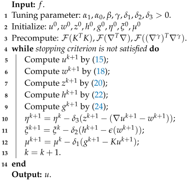
We summarize the FTGV-ADMM in Algorithm 1.
Algorithm 1:FTGV-ADMM algorithm to solve the proposed model.
Fractalfract 07 00756 i001
It is straightforward to see that FTGV-ADMM does not satisfy the convergence of ADMM (proven by Eckstein and Bertsekas [44]), since the fidelity term of problem (10) is non-convex. However, we can demonstrate the convergence of FTGV-ADMM by plotting the Energy and MSE values with respect to the iteration in Section 4.

3.2. Primal-Dual Algorithm

For the purpose of applying the Chambolle-Pock primal-dual (PD) algorithm [45,46], we need to rewrite the proposed model (10) as a minimax problem. Define:
A = I 0 ϵ , x = u w , x ¯ = u ¯ w ¯ , y = p q ,
and
F ( A x ) = α 1 u w 1 + α 0 ϵ ( w ) 1 , G ( x ) = β 2 γ ( K u ) γ f 2 2 ,
then the the proposed model (10) can be expressed as:
min x { F ( A x ) + G ( x ) } ;
it follows from the property of convex conjugate F , and can be defined as:
F ( y ) = 0 , if y 1 , + , otherwise .
Then the minimax problem of (10) is given as:
min u , w max p P , q Q { < u w , p > F ( p ) + < ϵ ( w ) , q > F ( q ) + β 2 γ ( K u ) γ f 2 2 } ,
where P and Q are, respectively, expressed as follows:
P = { p = ( p 1 , p 2 ) T | | p ( x ) | α 1 } , Q = q = q 11 q 12 q 21 q 22 | q α 0 ,
where the infinite norm is defined as | p ( x ) | = max i , j | p i , j | with | p i , j | = ( p 1 ) i , j 2 + ( p 2 ) i , j 2 . Similarly, it yields that q ( x ) = max i , j | q i , j | with
| q i , j | = ( q 11 ) i , j 2 + ( q 12 ) i , j 2 + ( q 21 ) i , j 2 + ( q 22 ) i , j 2 .
Applying the Chambolle-Pock algorithm for the minimax problem (26) yields the following iterative scheme:
p k + 1 = argmax p P { < u ¯ k w ¯ k , p > F ( p ) 1 2 σ p p k 2 2 } ; q k + 1 = argmax q Q { < ϵ ( w ¯ k ) , q > F ( q ) 1 2 σ q q k 2 2 } ; u k + 1 = argmin u { < u w ¯ k , p k + 1 > + β 2 γ ( K u ) γ f 2 + 1 2 τ u u k 2 2 } ; w k + 1 = argmin w { < u ¯ k + 1 w , p k + 1 > + < ϵ ( w ) , q k + 1 > + 1 2 τ w w k 2 2 } ; u ¯ k + 1 = 2 u k + 1 u k ; w ¯ k + 1 = 2 w k + 1 w k ;
where σ , τ are positive tuning parameters. Then, we obtain the respective closed-form solutions for subproblems in (27) one by one.
Specifically, for the p -subproblem and the q -subproblem, they have a closed-form solution, given by:
p k + 1 = Proj P [ p k + σ ( u ¯ k w ¯ k ) ] ,
q k + 1 = Proj Q [ q k + σ ϵ ( w ¯ k ) ] ,
where Proj P and Proj Q denote the Euclidean projection on the convex sets P and Q, respectively. They can be easily calculated by:
Proj P ( p ˜ ) = p ˜ max ( | p ˜ | / α 1 , 1 ) , Proj Q ( q ˜ ) = q ˜ max ( | q ˜ | / α 0 , 1 ) .
Solutions for the u-subproblem and the w-subproblem can be obtained by solving the corresponding Euler–Lagrange equation of the form:
u k + 1 = u k + τ [ div p k + 1 + β ( γ ) T γ K T ( K u k f ) ] ,
w k + 1 = w k + τ ( p k + 1 + div h q k + 1 ) ,
where K T is the adjoint operator of K and ( γ ) T is the adjoint operator of γ as above.
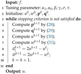
We summarize the FTGV-PD in Algorithm 2. The convergence of FTGV-PD is guaranteed by the following proposition and by plotting the energy and MSE values with respect to the iteration in Section 4.
Algorithm 2:FTGV-PD algorithm to solve the proposed model.
Fractalfract 07 00756 i002
The convergence result for the PD algorithm was proven by Chambolle and Pock in [47,48] when G ( x ) is convex. However, in our problem of the loss the convexity of the fidelity term G ( x ) , we cannot get the convergence of the PD algorithm to the problem (10) under normal circumstances unless G ( x ) is linearized, so we can solve the primal-dual problem:
min x max y { < A x , y > F ( y ) + < G ( x ¯ ) , x x ¯ > } ;
instead,
min x max y { < A x , y > F ( y ) + G ( x ) } .
We get the following convergence result for problem (32):
Proposition 2.
Let the sequence ( x k , y k ) be generated by (32). If we choose parameters τ and σ satisfying
τ σ L A 2 + τ L G 1 ,
where L A 2 = A 2 2 , L G is the Lipschitz constant of G, then ( x k , y k ) converges to the saddle point saddle-point of (10).
Proof of Proposition 2.
Based on the analysis, we only need to estimate the parameters L A and L G to enable the convergence of the proposed FTGV-PD algorithm, as well as to provide guidance on choosing the appropriate values of the parameters τ and σ .
The norm of A can be estimated as follows:
A x 2 2 = u w ϵ ( w ) 2 2 = I 0 ϵ u w 2 2 = I 0 ϵ 2 2 u w 2 2 .
Let x 2 2 = u w 2 2 = 1 ; then, we have A 2 = I 0 ϵ 2 < 12 (see details in [27]).
For the Lipschitz constant L G , it can be estimated by:
G ( u 1 ) G ( u 2 ) = β ( γ ) T γ K T K ( u 1 u 2 )
β ( γ ) T γ K T K u 1 u 2
β K 2 γ 2 u 1 u 2 ;
then, we get
L G β K 2 γ 2 .
Since k u 2 k 1 u 2 ([49]) and the GL definition of the fractional-order derivatives x γ u and y γ u can be described as the convolution of the weight coefficient ( 1 ) l C l γ (represented as k l ) and u, we, thus, have:
γ u 2 2 = x γ u 2 2 + y γ u 2 2 2 k 1 2 u 2 2 ,
where k = ( k 0 , w 1 , , k L 1 ) and k l = ( 1 ) l C l γ . For the special case of TV, i.e., γ = 1 , L = 2 , we have L 2 = 2 8 , which is consistent in [50]; hence, the upper bound of fractional order γ 2 is 8. □
Remark 4.
Proposition 2 is a special case of theorem 1 in Chambolle and Pock [48]. Thus, we can simply choose τ = 1 / ( L A + L G ) and σ = 1 / L A in our model.

4. Numerical Experiments

In this section, we will test the performance of the proposed model (2) with the PD algorithm and ADMM algorithm, and also compare with some efficient visual and analytical methods for image deblurring such as TGV [21], APE-TGV [28], D-TGV [33], BM3D [19], and NLTV [18]. To evaluate the restoration results, we use these quantitative measures, including the peak signal to noise ratio (PSNR), the mean square error (MSE), and the structural similarity (SSIM) metric, which are commonly used in image processing. The better quality image will have higher PSNR and SSIM, but lower MSE.
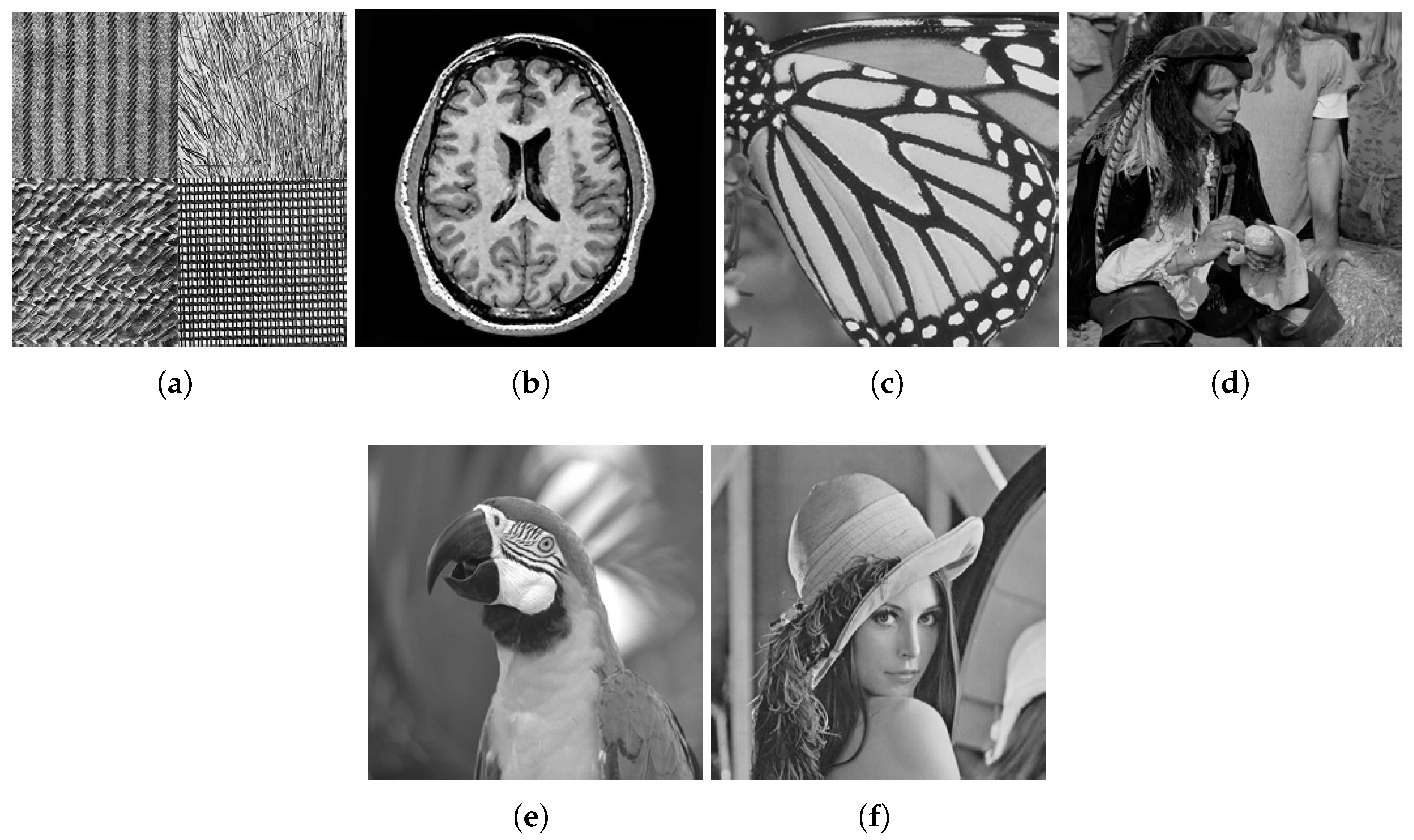
In experiments, we consider three common blur scenarios: motion blur, disk blur, and average blur. The motion blur, disk blur, and average blur are generated by the MATLAB built-in functions fspecial(‘motion’, 20, 50), fspecial(‘disk’, 5) and ones ( 9 ) / 81 , respectively. Except for the blur, we also add the Gaussian noise with standard deviation 0.1 to the blurry image. For illustration, six test images are presented in Figure 2 with different sizes. In all experiments, we terminate two algorithms when u k + 1 u k u k < 1 e 4 or Maxiter = 2000.

4.1. Comparison of Proposed Algorithms

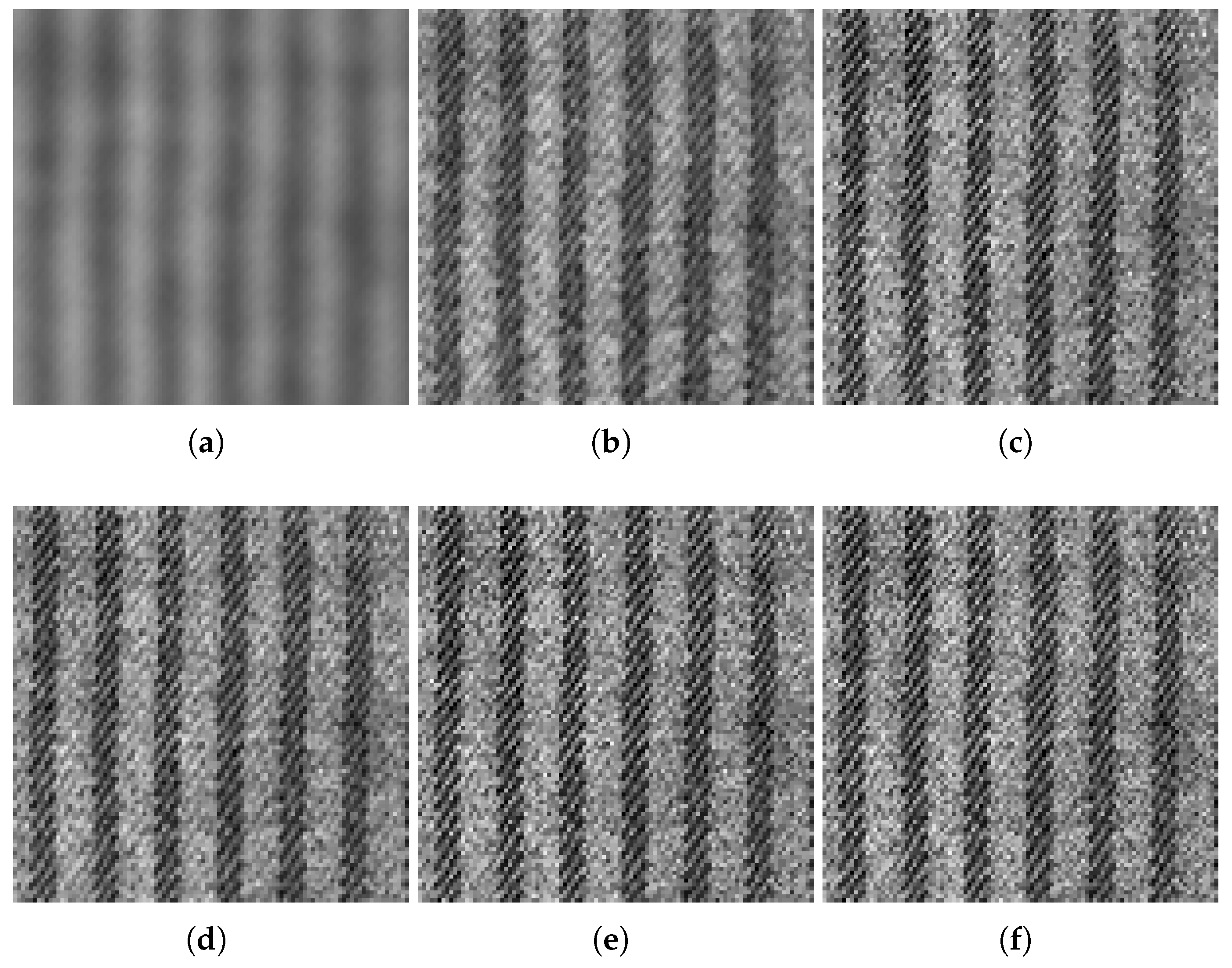
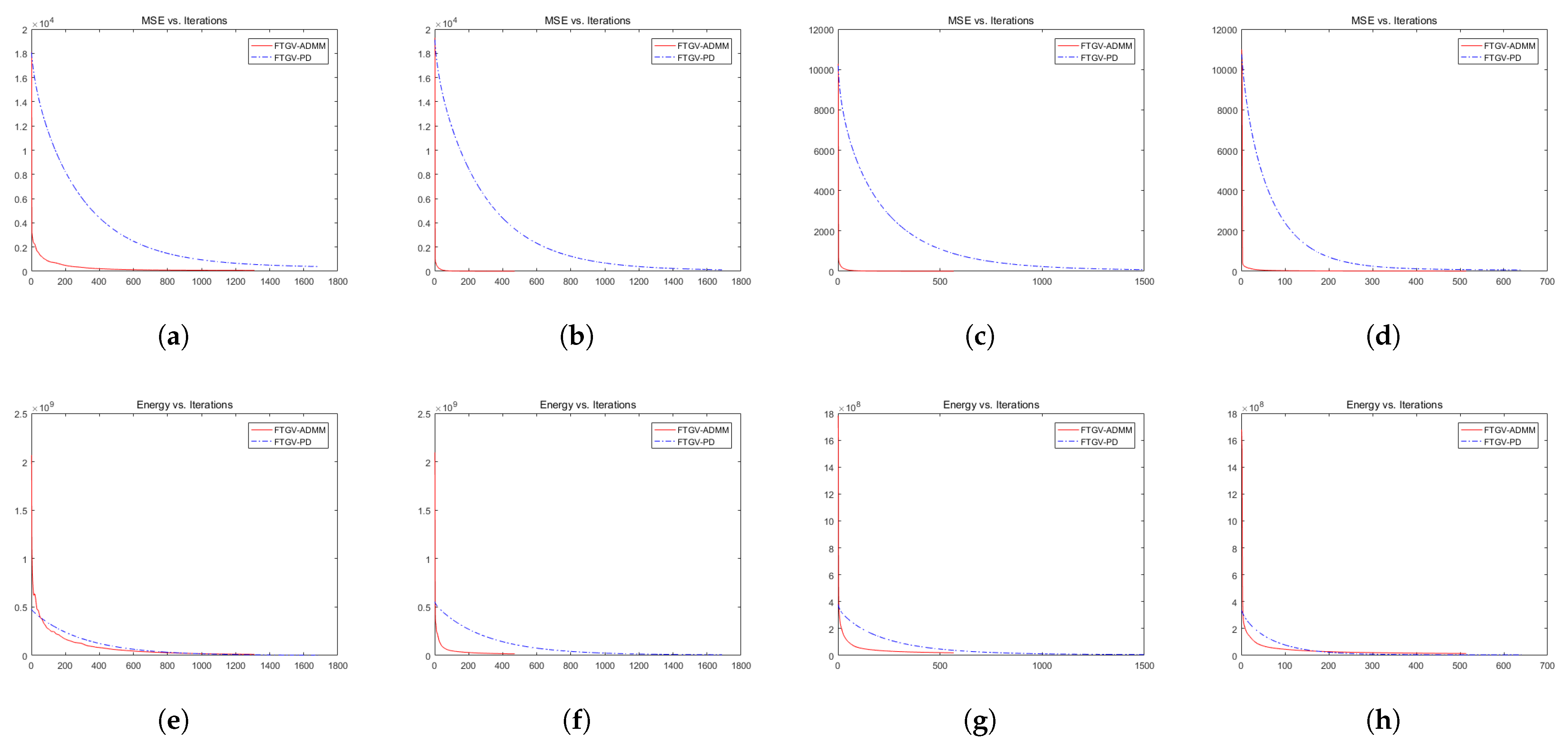
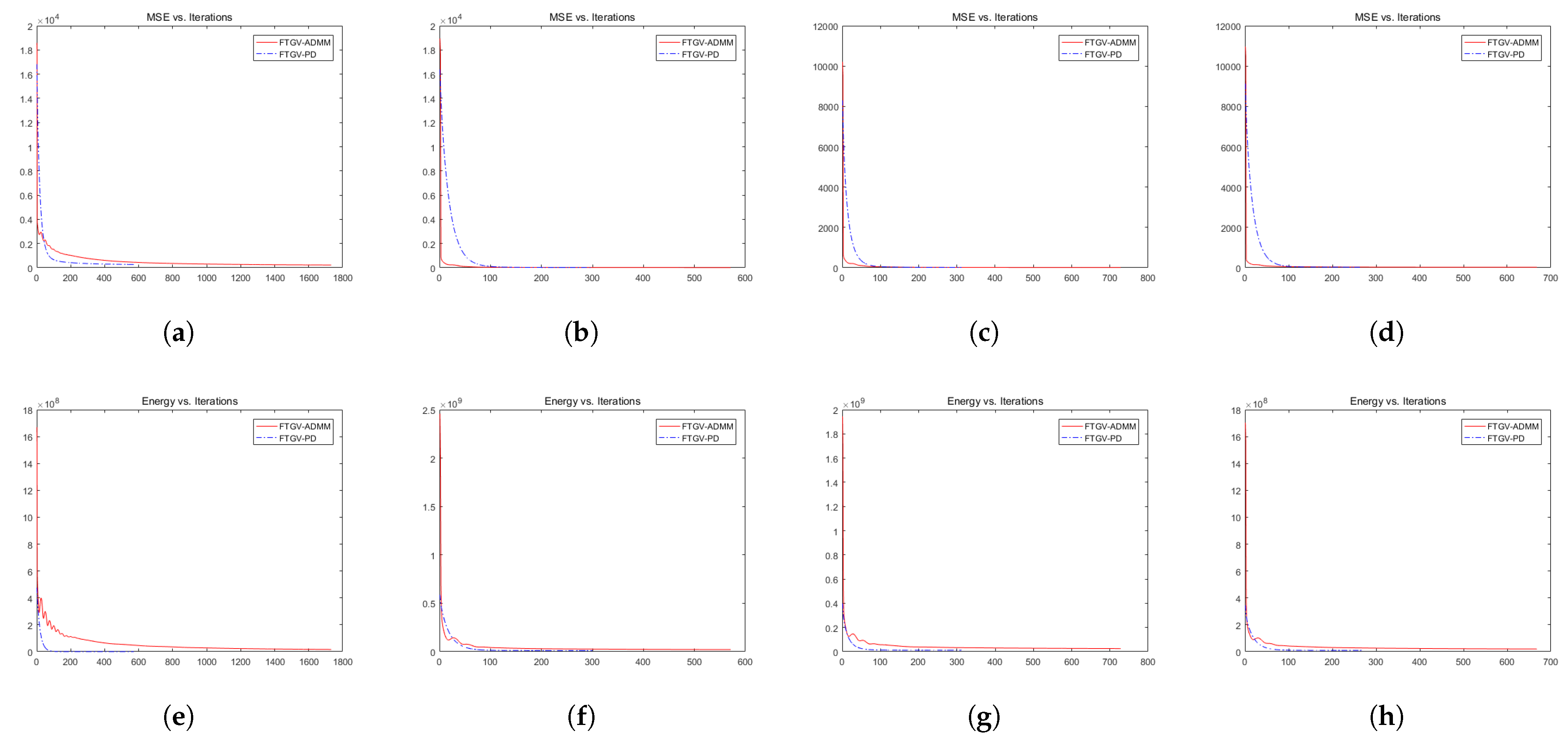
In this subsection, we compare the efficiency of the two proposed algorithms, FTGV-ADMM and FTGV-PD, by minimizing the same objective function (10). We optimize the algorithmic parameters for each algorithm to achieve higher PSNR improvement, which are listed in Table 1. The visual results are provided in Figure 3, Figure 4 and Figure 5, and Table 2 and Table 3 report the restoration results in terms of PSNR and SSIM values, along with other contrastive models. In addition, we plot the energy and MSE values with respect to the iteration in Figure 6 and Figure 7, and numerically demonstrate the convergence of each algorithm.
FTGV-ADMM does not satisfy the convergence of ADMM and, hence, for any penalty parameter, δ > 0 is not available. Actually, different choices about δ could influence the convergent speed of the algorithms. In our experiments, we set a satisfying rule of thumb for deblurring based on experience δ 1 = δ 2 = δ 3 = 0.01 .
In Table 2 and Table 3, we find that FTGV-ADMM has the highest PNSR value and competitive SSIM value for the texture image, butterfly image, brain image, and man image. FTGV-PD achieved slightly lower results than FTGV-ADMM in the PSNR value for disk blur and average blur. Unfortunately, we notice that FTGV-PD achieves bad results on motion blur for all test images, whether it is the texture image or natural images. In the visualization aspect, FTGV-ADMM achieves better recovery results than FTGV-PD overall.
The results provided in Figure 6 show that FTGV-ADMM has the lowest MSE value and the fewest iterations for all test images. On the contrary, FTGV-ADMM requires more iterations to obtain a smaller MSE. We observe that FTGV-ADMM is the fastest algorithm to minimize the energy because it costs less iterations. In terms of the disk blur presented in Figure 7, FTGV-PD owns the lowest MSE and less iterations for the texture image than FTGV-ADMM, but FTGV-ADMM has the fastest rate to obtain the lowest MSE for other three images. In addition, FTGV-PD is the fastest and best algorithm to minimize the energy. Although FTGV-ADMM has brief oscillations occurring during the descent process of energy, it did not affect the convergence result. For average blur, we get the same results as disk blur, so we omit it.
Next, we illustrate how the fractional order γ affects the image restoration referred to in Figure 8, which plots the largest PSNR value as a function of fractional order γ . The experimental results show that the fractional order γ in the fidelity term can avoid the staircase effect and get more detailed structures by choosing suitable orders.
From Figure 8, we can notice that for motion blur, the optimal order occurs at γ {0.1–0.8}; it is obvious that we get the lowest PSNR value when γ = 0.9 for all test images. For the disk blur, the optimal order occurs at γ = 0.8 , where test images have the highest PSNR value. The trend of curve of the average blur is roughly the same as with the disk blur, so it is omitted. Thus, we use the fractional orders γ = 0.7 or γ = 0.8 in our experiments to obtain a higher PSNR through simple adjustments.
Overall, as FTGV-ADMM involves the least number of parameters, and is suitable for all blur types and images compared to the FTGV-PD, we will use it for the rest of the experiments.

4.2. Comparison of Other TGV-Based Methods

To demonstrate that the model based on the fractional-order fidelity term has better capability in texture restoration than other fidelity-based models for images with rich texture and nature images, we compare the proposed model (2) with TGV [21], APE-TGV [28], and D-TGV [33] for three different blur kernels and the standard deviation 0.1 Gaussian noise. To fairly compare, the parameters of the comparison models are selected according to the recommendations of the corresponding paper through adjusting them appropriately to get better results and the best PSNR; the choice of parameters is listed in Table 1. We provide results in Figure 3, Figure 4 and Figure 5 and Table 2 and Table 3.
As we can see in Figure 3b, Figure 4b, and Figure 5b, TGV could not eliminate blur completely. The images restored by APE-TGV in Figure 3c, Figure 4c and Figure 5c were over-smoothed, in which the texture structure was lost. The D-TGV model has advantages in maintaining structures, but it tends to lose some texture details and create some artifacts. From Figure 3, Figure 4 and Figure 5, it is easy to find that the restoration result of D-TGV is visually inferior to APE-TGV for the texture image. This means that D-TGV and APE-TGV are imperfect under certain circumstances. However, the proposed model with the ADMM algorithm (FTGV-ADMM) overcome these drawbacks and gets a better balance between deblurring completely and restoring more image details; see Figure 3e, Figure 4e and Figure 5e.
Table 2 and Table 3 report that FTGV-ADMM is comprehensively superior to other models in terms of PSNR. For example, it is 8.4 db, 2.65 db, and 1.69 db higher than the TGV, APE-TGV, and D-TGV for the texture image damaged by motion blur. This demonstrates the superiority of FTGV-ADMM.

4.3. Comparison with BM3D and NLTV

In this subsection, we demonstrate the performance of FTGV-ADMM with the famous blockmatching and 3D filtering (BM3D) method and the nonlocal TV (NLTV) for solving the image deblurring problem. In this paper, we use the preconditioned Bregmanized operator splitting (PBOS) method proposed by Zhang and Burger et al. [18]. Other parameters of the method are selected as suggested by the authors, but the regularization parameter μ is adjusted to obtain the highest PSNR value.
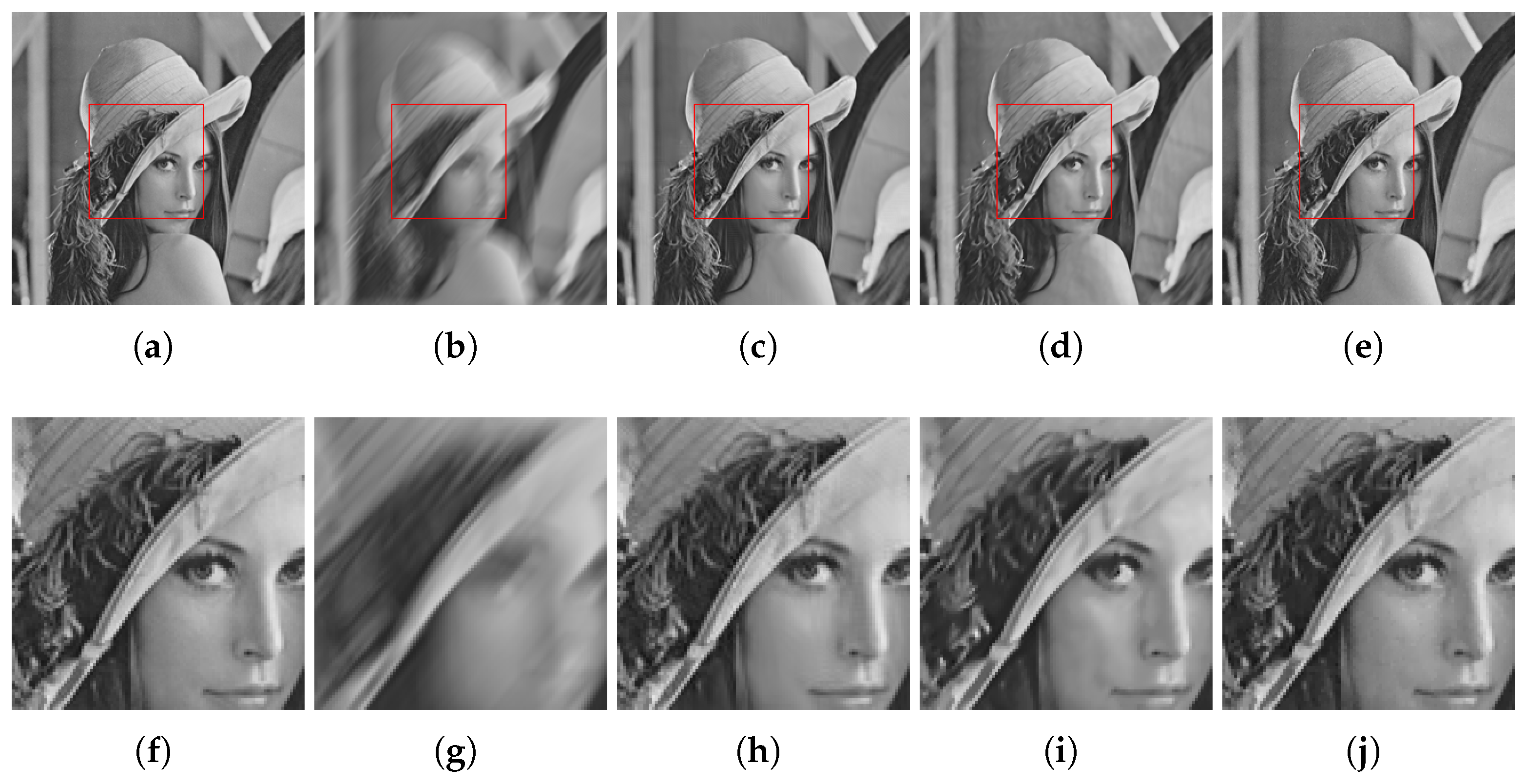
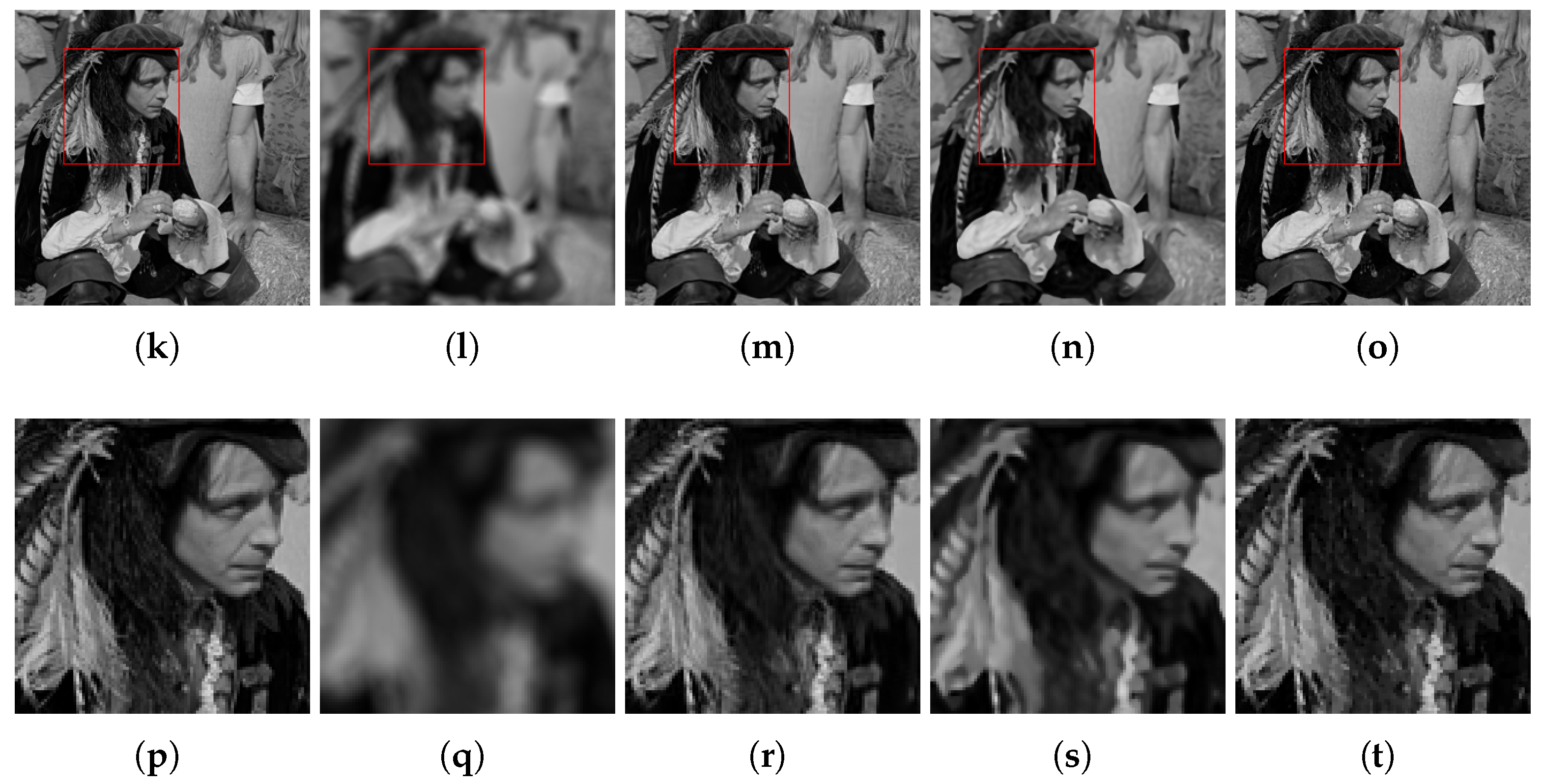
Four images are used in this example. They are corrupted by motion blur and disk blur and Gaussian noise. The experimental results are displayed in Figure 9, Figure 10, Figure 11 and Figure 12 and Table 4.
From Table 4, we can see that FTGV-ADMM achieves the best PSNR and SSIM values, which are far higher than the BM3D and NLTV methods. The visual quality of the deblurred results by the NLTV method is too over-smooth, and it produces obvious artifacts; see enlarged zoom Figure 9i, Figure 10i, Figure 11i and Figure 12i. The BM3D method is one of the best existing deblurring methods for Gaussian blurs and out-of-focus blurs, but the restoration image is still a little smooth and many details have been lost, which can be seen in the enlarged, zoomed Figure 9h, Figure 10h, Figure 11h and Figure 12h. Most importantly, FTGV-ADMM overcomes these difficulties and achieves higher visual quality.

5. Conclusions

The paper studies a novel image deblurring model that is applicable to three different blur kernels. The new model contains a fidelity term in fractional-order derivative space, which has the ability to preserve details, eliminate the staircase effect, and has a total generalized variation (TGV) regularization term. We propose two optimal numerical algorithms based on the PD method and the ADMM method to overcome the non-convex and non-differentiability of the new variational model. The experiment results show that our model is both quantitatively and qualitatively better than other advanced models.

Author Contributions

Conceptualization, J.G. and Z.G.; methodology, all authors; software, J.G., W.Y.; validation, J.G., W.Y. and Z.G.; formal analysis, J.G. and W.Y.; investigation, J.S., J.G. and W.Y.; resources, J.G. and Z.G.; data curation, J.G. and W.Y.; writing—original draft preparation, J.G. and W.Y.; writing—review and editing, J.G., Z.G., J.S. and W.Y.; visualization, J.G. and Z.G.; supervision, J.G., J.S. and Z.G.; project administration, Z.G., J.S. and W.Y.; funding acquisition, Z.G. and W.Y. All authors have read and agreed to the published version of the manuscript.

Funding

This work is supported by the National Natural Science Foundation of China (12301536, 12171123, 11971131, 12271130, U21B2075, 11871133, 61873071, 51476047), the Natural Science Foundation of Heilongjiang Province of China (LH2021A011), China Postdoctoral Science Foundation (2020M670893), the Fundamental Research Fund for the Central Universities (HIT. NSRIF202302, 2022FRFK060020, HIT. NSRIF202202), and the China Society of Industrial and Applied Mathematics Young Women Applied Mathematics Support Research Project.

Data Availability Statement

The data used to support the findings of this study are available from the corresponding author upon request.

Conflicts of Interest

The authors declare that they have no conflict of interest.

References

  1. Kundur, D.; Hatzinakos, D. Blind image deconvolution. IEEE Signal Process. Mag. 1996, 13, 43–64. [Google Scholar] [CrossRef]
  2. Kundur, D.; Hatzinakos, D. A novel blind deconvolution scheme for image restoration using recursive filtering. IEEE Trans. Signal Process. 1998, 46, 375–390. [Google Scholar] [CrossRef]
  3. Lehr, J.; Sibarita, J.-B.; Chassery, J.-M. Image restoration in X-ray microscopy: PSF determination and biological applications. IEEE Trans. Image Process. 1998, 7, 258–263. [Google Scholar] [CrossRef] [PubMed]
  4. Qin, F.; Min, J.; Guo, H. A blind image restoration method based on PSF estimation. In Proceedings of the IEEE 2009 WRI World Congress on Software Engineering, Xiamen, China, 19–21 May 2009; Volume 2, pp. 173–176. [Google Scholar]
  5. Erler, K.; Jernigan, E. Adaptive image restoration using recursive image filters. IEEE Trans. Signal Process. 1994, 42, 1877–1881. [Google Scholar] [CrossRef]
  6. Liu, Z.; Caelli, T. A sequential adaptive recursive filter for image restoration. Comput. Vis. Graph. Image Process. 1988, 44, 332–349. [Google Scholar] [CrossRef]
  7. Rudin, L.; Osher, S.; Fatemi, E. Nonlinear total variation based noise removal algorithms. Phys. D Nonlinear Phenom. 1992, 60, 259–268. [Google Scholar] [CrossRef]
  8. Rudin, L.; Osher, S. Total variation based image restoration with free local constraints. In Proceedings of the 1st International Conference on Image Processing, Austin, TX, USA, 13–16 November 1994; pp. 31–35. [Google Scholar]
  9. Lysaker, M.; Lundervold, A.; Tai, X.C. Noise removal using fourth-order partial differential equation with applications to medical magnetic resonance images in space and time. IEEE Trans. Image Process. 2003, 12, 1579–1590. [Google Scholar] [CrossRef]
  10. Deng, L.; Fang, Q.; Zhu, H. Image denoising based on spatially adaptive high order total variation model. In Proceedings of the International Congress on Image and Signal Processing, BioMedical Engineering and Informatics, Datong, China, 15–17 October 2016; pp. 212–216. [Google Scholar]
  11. Adam, T.; Paramesran, R. Hybrid non-convex second-order total variation with applications to non-blind image deblurring. Signal Image Video Process. 2020, 14, 115–123. [Google Scholar] [CrossRef]
  12. He, C.; Hu, C.; Zhang, W.; Shi, B. A fast adaptive parameter estimation for total variation image restoration. IEEE Trans. Image Process. 2014, 23, 4954–4967. [Google Scholar] [CrossRef]
  13. Liu, J.; Huang, T.Z.; Selesnick, I.W.; Lv, X.G.; Chen, P.Y. Image restoration using total variation with overlapping group sparsity. Inf. Sci. 2015, 295, 232–246. [Google Scholar] [CrossRef]
  14. Carlavan, M.; Blanc-Féraud, L. Sparse Poisson noisy image deblurring. IEEE Trans. Image Process. 2012, 21, 1834–1846. [Google Scholar] [CrossRef] [PubMed]
  15. Bai, J.; Feng, X.C. Fractional-order anisotropic diffusion for image denoising. IEEE Trans. Image Process. 2007, 16, 2492–2502. [Google Scholar] [CrossRef]
  16. Chowdhury, M.R.; Qin, J.; Lou, Y. Non-blind and blind deconvolution under Poisson noise using fractional-order total variation. J. Math. Imaging Vision 2020, 62, 1238–1255. [Google Scholar] [CrossRef]
  17. Gilboa, G.; Osher, S. Nonlocal operators with applications to image processing. Multiscale Model. Simul. 2009, 7, 1005–1028. [Google Scholar] [CrossRef]
  18. Zhang, X.; Burger, M.; Bresson, X.; Osher, S. Bregmanized nonlocal regularization for deconvolution and sparse reconstruction. SIAM J. Imaging Sci. 2010, 3, 253–276. [Google Scholar] [CrossRef]
  19. Dabov, K.; Foi, A.; Katkovnik, V.; Egiazarian, K. Image restoration by sparse 3-D transformdomain collaborative filtering. SPIE Electron. Imaging 2008, 6812, 62–73. [Google Scholar]
  20. Danielyan, A.; Katkovnik, V.; Egiazarian, K. BM3D frames and variational image deblurring. IEEE Trans. Image Process. 2012, 21, 1715–1728. [Google Scholar] [CrossRef]
  21. Bredies, K.; Kunisch, K.; Pock, T. Total Generalized Variation. SIAM J. Imaging Sci. 2010, 3, 492–526. [Google Scholar] [CrossRef]
  22. Liu, X. Augmented Lagrangian method for total generalized variation based Poissonian image restoration. Comput. Math. Appl. 2016, 71, 1694–1705. [Google Scholar] [CrossRef]
  23. Liu, X. Total generalized variation and wavelet frame-based adaptive image restoration algorithm. Vis. Comput. 2019, 35, 1883–1894. [Google Scholar] [CrossRef]
  24. Shao, W.Z.; Wang, F.; Huang, L.L. Adapting total generalized variation for blind image restoration. Multidimens. Syst. Signal Process. 2019, 30, 857–883. [Google Scholar] [CrossRef]
  25. Gao, Y.; Liu, F.; Yang, X. Total generalized variation restoration with non-quadratic fidelity. Multidimens. Syst. Signal Process. 2018, 29, 1459–1484. [Google Scholar] [CrossRef]
  26. Knoll, F.; Bredies, K.; Pock, T.; Stollberger, R. Second order total generalized variation (TGV) for MRI. Magn. Reson. Med. 2011, 65, 480–491. [Google Scholar] [CrossRef]
  27. Bredies, K.; Valkonen, T. Inverse problems with second-order total generalized variation constraints. arXiv 2020, arXiv:2005.09725. [Google Scholar]
  28. He, C.; Hu, C.; Yang, X. An adaptive total generalized variation model with augmented lagrangian method for image denoising. Math. Probl. Eng. 2014, 2014, 157893. [Google Scholar] [CrossRef]
  29. Bredies, K. Recovering Piecewise Smooth Multichannel Images by Minimization of Convex Functionals with Total Generalized Variation Penalty; Springer: Berlin/Heidelberg, Germany, 2014; pp. 44–77. [Google Scholar]
  30. Tirer, T.; Giryes, R. Image restoration by iterative denoising and backward projections. IEEE Trans. Image Process. 2019, 28, 1220–1234. [Google Scholar] [CrossRef] [PubMed]
  31. Ren, D.; Zhang, H.; Zhang, D. Fast total-variation based image restoration based on derivative alternated direction optimization methods. Neurocomputing 2015, 170, 201–212. [Google Scholar] [CrossRef]
  32. Patel, V.M.; Maleh, R.; Gilbert, A.C.; Chellappa, R. Gradient-based image recovery methods from incomplete Fourier measurements. IEEE Trans. Image Process. 2011, 21, 94–105. [Google Scholar] [CrossRef]
  33. Zou, T.; Li, G.; Ma, G.; Zhao, Z.; Li, Z. A derivative fidelity-based total generalized variation method for image restoration. Mathematics 2022, 10, 3942. [Google Scholar] [CrossRef]
  34. Podlubny, I. Fractional Differential Equations, An introduction to fractional derivatives, frac-tional differential equations, to methods of their solution and some of their applications. In Mathematics in Science and Engineering; Academic Press, Inc.: San Diego, CA, USA, 1999. [Google Scholar]
  35. Guo, Z.; Yao, W.; Sun, J.; Wu, B. Nonlinear fractional diffusion model for deblurring images with textures. Inverse Probl. Imaging 2019, 13, 1161–1188. [Google Scholar] [CrossRef]
  36. Yao, W.; Guo, Z.; Sun, J.; Wu, B.; Gao, H. Multiplicative Noise Removal for Texture Images Based on Adaptive Anisotropic Fractional Diffusion Equations. SIAM J. Imaging Sci. 2019, 12, 839–873. [Google Scholar] [CrossRef]
  37. Dyda, B.; Ihnatsyeva, L.; Vähäkangas, A.V. On improved fractional Sobolev-Poincaré inequalities. Ark. Mat. 2016, 54, 437–454. [Google Scholar] [CrossRef]
  38. Hurri-Syrjnen, R.; Vhkangas, A.V. On fractional Poincaré inequalities. J. Anal. Mathématique 2011, 120, 85–104. [Google Scholar] [CrossRef]
  39. Jonsson, A.; Wallin, H. A Whitney extension theorem in Lp and Besov spaces. Ann. Inst. Fourier. 1978, 28, 139–192. [Google Scholar] [CrossRef]
  40. Adams, R.A. Sobolev Spaces; Pure and Applied Mathematics; Academic Press: San Diego, CA, USA, 1975; p. 65. [Google Scholar]
  41. Bourgain, J.; Brezis, H.; Mironescu, P. Another look at Sobolev spaces. Optimal. In Control and Partial Differential Equations; IOS Press: Amsterdam, The Netherlands, 2001; pp. 439–455. [Google Scholar]
  42. Meerschaert, C.; Tadjeran, M.M. Finite difference approximations for fractional advectiondispersion equations. J. Comput. Appl. Math. 2004, 172, 65–77. [Google Scholar] [CrossRef]
  43. Boyd, S.; Parikh, N.; Chu, E.; Peleato, B.; Eckstein, J. Distributed optimization and statistical learning via the alternating direction method of multipliers. Found. Trends Mach. Learn. 2011, 3, 1–122. [Google Scholar] [CrossRef]
  44. Eckstein, J.; Bertsekas, D. On the Douglas-Rachford splitting method and the proximal point algorithm for maximal monotone operators. Math. Program. 1992, 55, 293–318. [Google Scholar] [CrossRef]
  45. Zhu, M.; Chan, T.F. An efficient primal-dual hybrid gradient algorithm for total variation image restoration. UCLA CAM Rep. 2008, 34, 8–34. [Google Scholar]
  46. Esser, E.; Zhang, X.; Chan, T. A general framework for a class of first order primal-dual algorithms for TV minimization. UCLA CAM Rep. 2009, 9, 67. [Google Scholar]
  47. Chen, Y.; Lan, G.; Ouyang, Y. Optimal primalšCdual methods for a class of saddle pont problems. SIAM J. Optim. 2014, 24, 1779–1814. [Google Scholar]
  48. Chambolle, A.; Pock, T. On the ergodic convergence rates of a first-order primalšCdual algorithm. Math. Program. 2016, 159, 253–287. [Google Scholar] [CrossRef]
  49. Bahouri, H.; Chemin, J.Y.; Danchin, R. Fourier Analysis Nonlinear Partial Differential Equations; Springer: Berlin, Germany, 2011. [Google Scholar]
  50. Chambolle, A. An algorithm for total variation minimization and applications. J. Math. Imaging Vision 2004, 20, 89–97. [Google Scholar]
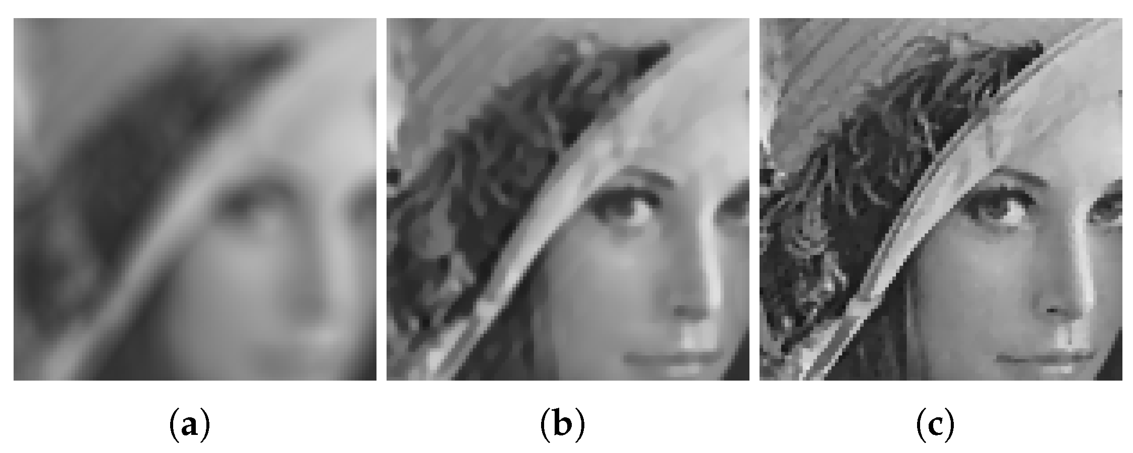
Figure 1. Visualization in zoom for Lena image. (a) Noisy blurred image (disk blur with radius 5 and a Gaussian noise with σ = 0.1 ), (b) deblurred image of integer model, (c) deblurred image of fractional model.
Fractalfract 07 00756 g001
Figure 2. Test images: (a) synthetic texture ( 256 × 256 ), (b) brain ( 300 × 281 ), (c) butterfly ( 256 × 256 ), (d) man ( 256 × 256 ), (e) parrot ( 256 × 256 ), and (f) Lena ( 256 × 256 ).
Fractalfract 07 00756 g002
Figure 3. (a) Motion blurred image; (bf) deblurred images by TGV, APE-TGV, D-TGV, FTGV-ADMM, and FTGV-PD.
Fractalfract 07 00756 g003
Figure 4. (a) Disk blurred image; (bf) deblurred images by TGV, APE-TGV, D-TGV, FTGV-ADMM, and FTGV-PD.
Fractalfract 07 00756 g004
Figure 5. (a) Average blurred image; (bf) deblurred images by TGV, APE-TGV, D-TGV, FTGV-ADMM, and FTGV-PD.
Fractalfract 07 00756 g005
Figure 6. First row: iteration-varying of MSE for motion blur. (a) texture, (b) butterfly, (c) brain, (d) man. Second row: iteration-varying of energy for motion blur. (e) texture, (f) butterfly, (g) brain, (h) man.
Fractalfract 07 00756 g006
Figure 7. First row: iteration-varying of MSE for disk blur. (a) texture, (b) butterfly, (c) brain, (d) man. Second row: iteration-varying of Energy for disk blur. (e) texture, (f) butterfly, (g) brain, (h) man.
Fractalfract 07 00756 g007
Figure 8. The influence of the fractional-orders γ on restored results. (a) PSNR values for different γ on motion blur. (b) PSNR values for different γ on disk blur.
Fractalfract 07 00756 g008
Figure 9. Performance comparison of the proposed method with BM3D and NLTV for the Lena image. The red squares are marked for zooming. First row: (a) original image; (b) motion blurred image; (ce) deblurred image by BM3D, NLTV, and FTGV-ADMM. Second row: (fj) corresponding enlarged version of (ae).
Fractalfract 07 00756 g009
Figure 10. Performance comparison of the proposed method with BM3D and NLTV for the parrot image. The red squares are marked for zooming. First row: (a) original image; (b) disk blurred noisy image; (ce) deblurred image by BM3D, NLTV, and FTGV-ADMM. Second row: (fj) corresponding enlarged version of (ae).
Fractalfract 07 00756 g010aFractalfract 07 00756 g010b
Figure 11. Performance comparison of the proposed method with BM3D and NLTV for the man image. The red squares are marked for zooming. First row: (a) original image; (b) disk blurred noisy image; (ce) deblurred image by BM3D, NLTV, and FTGV-ADMM. Second row: (fj) corresponding enlarged version of (ae).
Fractalfract 07 00756 g011
Figure 12. Performance comparison of the proposed method with BM3D and NLTV for the butterfly image. The red squares are marked for zooming. First row: (a) original image; (b) motion blurred noisy image; (ce) deblurred image by BM3D, NLTV, and FTGV-ADMM. Second row: (fj) corresponding enlarged version of (ae).
Fractalfract 07 00756 g012
Table 1. The parameter values for numerical experiments on all test images.
ModelImage TypeIIIIII
TGV( α 1 , α 0 , β )All images(1,2,35)(1,2,35)(1,2,35)
APE-TGV ( α 1 , α 0 , β )All images(1,3,0.3)(1,3,0.3)(1,3,0.3)
DTGV ( α 1 , α 0 , μ )Texture image(1,2,2000)(1,2,2000)(1,2,2000)
Other images(5,10,2000)(5,10,2000)(5,10,2000)
FTGV-ADMMAll images(0.1,0.2,0.7,5000)(0.1,0.2,0.7,5000)(0.1,0.2,0.7,5000)
FTGV-PDTexture image(0.1,0.2,0.8,150)(0.1,0.2,0.8,2500)(0.1,0.2,0.8,2500)
Other images(5,10,0.8,150)(10,20,0.8,2500)(10,20,0.8,2500)
Table 2. Quantitative comparison with three blur kernels. Bold values indicate the best result.
FigureMethodsIIIIII
PSNR/SSIMPSNR/SSIMPSNR/SSIM
TextureTGV22.59/0.893718.91/0.743619.82/0.6964
APE-TGV28.34/0.972925.83/0.933524.01/0.8763
D-TGV29.03/0.977624.17/0.916222.77/0.8588
FTGV-ADMM 30 . 99 / 0 . 9850 27 . 66 / 0 . 9536 25 . 06 /0.9080
FTGV-PD24.75/0.944226.70/0.950224.75/ 0 . 9174
ButterflyTGV26.74/0.882627.30/0.906925.93/0.8759
APE-TGV37.01/0.981434.29/0.974733.12/0.9668
D-TGV35.72/0.966534.20/0.962731.70/0.9477
FTGV-ADMM 38 . 48 /0.9812 35 . 24 /0.9741 34 . 09 / 0 . 9688
FTGV-PD26.38/0.928534.67/0.968132.58/0.9571
Table 3. Quantitative comparison with three blur kernels. Bold values indicate the best result.
FigureMethodsIIIIII
PSNR/SSIMPSNR/SSIMPSNR/SSIM
BrainTGV30.45/0.817328.96/0.921928.26/0.8959
APE-TGV39.90/0.989937.07/ 0 . 9861 34.53/ 0 . 9765
D-TGV38.72/0.909736.67/0.958333.76/0.9512
FTGV-ADMM 41 . 88 /0.9747 38 . 26 /0.9721 36 . 45 /0.9729
FTGV-PD29.67/0.796737.11/0.975334.26/0.9656
ManTGV28.57/0.856627.24/0.822926.54/0.8000
APE-TGV35.71/0.964133.26/0.940931.42/0.9225
D-TGV36.50/0.964333.78/0.944431.98/0.9228
FTGV-ADMM 37 . 50 / 0 . 9710 34 . 28 / 0 . 9492 32 . 60 / 0 . 9335
FTGV-PD29.28/0.865733.35/0.939531.66/0.9169
Table 4. Quantitative comparison of BM3D, NLTV, and FTGV-ADMM.
FigureMethodsPSNRSSIM
Figure 9BM3D36.670.9563
NLTV33.760.9392
FTGV-ADMM38.660.9761
Figure 10BM3D37.680.9575
NLTV35.310.9467
FTGV-ADMM38.650.9717
Figure 11BM3D32.210.9183
NLTV29.120.8251
FTGV-ADMM34.280.9492
Figure 12BM3D33.650.9580
NLTV30.470.9219
FTGV-ADMM38.480.9812
Disclaimer/Publisher’s Note: The statements, opinions and data contained in all publications are solely those of the individual author(s) and contributor(s) and not of MDPI and/or the editor(s). MDPI and/or the editor(s) disclaim responsibility for any injury to people or property resulting from any ideas, methods, instructions or products referred to in the content.