1. Introduction and Preliminaries
Convex analysis is regarded as the most fundamental branch of mathematical analysis. It has gained effective attention due to its major role in the development of both pure and applied mathematics. Convexity and its consequences provide both a geometrical and analytical approach to solving a problem. The role of convexity is unforgettable in linear algebra, topology, and functional analysis, especially separation axioms, fixed point theory, engineering, and economics as well. Firstly, in 1905, Jensen made the theory function much more interesting by introducing the concept of convex mappings on the basis of a convex set. One would like to characterize it by functions and their derivatives, as a positive second derivative indicates the convexity of functions. It is closely related to the theory of optimization, especially in linear programming. Convex mappings are often utilized to derive a feasible solution, and they provide unique minima.
The theory of inequalities is a broad discipline of research in mathematical analysis, and it has several applications in numerous areas of mathematics, physics, and engineering. Strong linkages between this theory and other disciplines, including functional analysis, approximation theory, probability theory, and information theory, have been found. As a consequence of its influence on applied mathematics, this field’s prominence will rise in the future. Theory convex functions have played a significant role in the development of the theory of inequalities. Many inequalities can be obtained directly by utilizing the notion of convexity such as Jensen’s inequality, HH inequality, Young’s inequality, etc. In this regard, we recall the well-known inequality due to Hermite and Hadamard separately. Let
be a convex function with
, then
Through the utilization of the above inequality, one can check the concavity of the different mappings. For more detail about this, see [
1,
2].
Recently, the concept of convexity has been refined and extended by using novel and innovative ideas, especially by making use of weighted means, for example, harmonic, geometric, and
P convexity based on weighted harmonic mean, weighted geometric mean, and generalized weighted
p mean, respectively. In 2019, Wu et al. [
3] explored the new class of convexity by utilizing the quasi-arithmetic mean, which is described as:
Definition 1. Let be a strictly continuous function. Then, is said to be ⋎-convex set with respect to ⋎ if: Now, we revisit the class ⋎-convex function, which is studied in [
3].
Definition 2. A function is said to be a ⋎-convex function with respect to a strictly monotonic continuous function ⋎ if In 2021, Kashuri et al. [
4] discuss the ⋎ invex set and exponential preinvex functions, which are given by:
Definition 3. Let be a bifunction and ⋎ be a strictly monotonic continuous function. Then, k is said to be K⋎-invex set, if Next, we have an exponential ⋎-exponential preinvex function.
Definition 4 ([
4]).
Let be a bifunction, ⋎ be a strictly monotonic continuous function, and β be non-positive. Then, is said to be ⋎-exponential preinvex function if Now, we present Condition C.
Let be an invex set with respect to a bifunction . Then, satisfies the condition c for any and if
- 1.
- 2.
In set-valued analysis, we deal with multi-valued functions, and I.V. analysis is a sub-discipline of this subject. Initially, interval analysis was used to calculate the error estimates of finite machines. As in daily life processes, if we assign a single value to any variable, then the chance of error increases; to overcome this deficiency, a numerical single number is replaced by interval numbers. Moore wrote some interesting books on interval analysis, which revealed new directions in executing this theory, and proposed some applications for computer programming and error analysis. After remarkable and applicable work due to Moore, many authors have shown their interest in the field and used it in different directions. I.V. techniques are used to investigate dynamic systems of differential equations, fluid mechanics, combinatorics, neural networking, and inequalities (see [
5]). In the continuation, Breckner [
6] purported the idea of convexity from the perspective of set-valued mappings, which are given as:
Definition 5. Let , which is said to be an I.V. convex function if The space of intervals is denoted by . Sadowska was the first who examined the classical HH-type inequality through convex set-valued mappings. This is stated as:
Let
be an interval-valued convex mapping defined over the interval
and
together with
.
If
is set of all partitions of
and
is the set of all points
P such that
, then
is called an interval Riemann integrable on
if there exist
and for each
there exists
such that
where
is the Riemann sum of
with respect to
. Relation (
1) shows that
K is the
-integral of
and given by
Definition 6. Let , which is said to be a generalized invex set with respect to mapping , and ⋎ be a monotonically continuous function if Theorem 1. Let be an I.V. function such that if and only if and Next, we give the I.V. analog of AB-fractional operators.
Definition 7. The fractional integral concerned with the new fractional derivative with the nonlocal kernel of a mapping is described as: Similarly, the right-sided AB-operator is stated as: Here, is the gamma function. is called the normalization function.
For more detail about fractional calculus see [
7].
Assume that is an I.V. mapping. Now, we revisit I.V. fractional -operators, which are defined as:
Definition 8. , and both mappings and are Riemann integrable defined on the interval . Then,andwith and as the normalization function. We clearly see thatand Recently, several inequalities have been extended and refined by implementing the I.V. mappings and ordering relations defined over interval numbers. In this regard, Chalco-Cano et al. [
8,
9] computed the familiar Ostrowski’s integral inequality via I.V. mappings and Hukuhara derivatives and concluded the applicable utility of the main outcomes in a numerical analysis, respectively. In 2017, Costa et al. [
10] explored the novel integral inequalities by applying the mappings defined over fuzzy numbers. In the continuation, Flores et al. [
11] computed the new variants of integral inequalities associated with I.V. mappings. In [
12], the authors investigated the integral inequalities of HH involving preinvex I.V. mappings. Zhao et al. [
13,
14] established the Jensen’s and HH-type containment involving a general class of I.V. convexity, which is referred to as
-I.V. mapping and Chebyshev-type inequalities, respectively. Fractional calculus has contributed extraordinary impacts on the growth of integral inequalities. In 2012, Sarikaya et al. [
15] made the first successful attempt to establish fractional counterparts of HH-type inequalities, essentially considering integral fractional operators. After this, several inequalities have been improved by using fractional tools, and this is still a very active field of research. In [
16,
17], Mohammad et al. examined the new tempered Hermite-Hadmard-like inequalities and presented some applications as well as fractional mid-point-like inequalities in the frame of fractional calculus. In [
18], Akdemir et al. analyzed the Chebyshev-like inequalities through unified fractional operators. Set et al. [
19] concluded with the inequalities involving AB-fractional integral operators and differentiability of convex mappings. In 2020, Budak et al. [
20] studied the interval-valued fractional operators to explore the HH-type inequalities. Kara et al. [
21] used the conception of interval-valued coordinated convexity and new double fractional operators to prove some HH-type inequalities. Recently, Bin-Mohsin et al. [
22] introduced the notion of interval-valued coordinated harmonically convex mappings and double fractional operators involving the generalized Mittag-Leffler function introduced by Raina as a kernel to extract some novel fractional versions of HH-type inequalities. Zhou et al. [
23] explored the trigonometric convex functions with exponential weight to formulate some new variants of HH-like inequalities. In [
24], they discussed trigonometric convexity and related integral containment, implementing the fuzzy ordered relation. In [
25], Kalsoom et al. used the idea of I.V. convexity and
calculus to establish some new refinements of existing results. In [
26], the authors introduced the concept of the fuzzy interval-valued bi-convex function to obtain some HH-like inequalities. In [
27,
28], the authors obtained fractional variants of Hermite–Hadamard-type inequalities for interval-coordinated convex functions and product inequalities of Hermite–Hadamard-type inequalities, respectively. In [
29], they concluded with new Hermite–Hadamard-type inequalities involving interval-valued convexity and generalized quantum calculus. For more detail and recent developments see [
30,
31,
32,
33,
34].
The main focus of the proceeding study is to obtain new generic inclusion relations of the HH-type by invoking AB-fractional concepts. First of all, we develop a novel class of convexity based on the bi-function and monotonically continuous function ⋎ in interval analysis. The novelty of this study is that by applying different values of and , several existing and new fractional counterparts can be deduced. Additionally, we validated our theoretical outcomes via numerical simulations. To the best of our knowledge, these results are more beneficial for acquiring variants of I.V. HH-type inequalities for several classes of convexity. The structure of the paper consists of two sections: in the first segment of the study, we recall some facts relative to convexity and fractional calculus, and some history of the problem is explained. In the second section, we introduce the newly proposed class of convexity, and its consequences and applications in integral inequalities are provided. Later on, concluding remarks are added.
2. Main Results
Now, we define I.V. pre-invex mappings.
Definition 9. Let be a non-negative mapping with , then is called I.V. pre-invex mappings, satisfying the condition if and . Now, we discuss some special cases of Definition 2.
Choosing
, we acquire a fresh class ⋎ I.V. pre-invex function:
Choosing
and
, we then obtain a class of I.V. harmonically pre-invexity:
Choosing
and
, we then obtain a class of I.V.
P pre-invex functions:
Choosing
and
, we then obtain a class of I.V. log-exponential pre-invex functions:
Remark 1. Choosing , we then obtain the definition of classical I.V. pre-invex functions.
Definition 10. Choosing in Definition 2, we acquire a fresh class I.V. -pre-invex function Now, we investigate some special cases of Definition 10.
Setting , we then obtain I.V. harmonically s pre-invex functions, which follow as Setting , , we then obtain I.V. pre-invex functions, which follow as Choosing and , we then obtain a class of I.V. log-exponential s pre-invex functions:
Definition 11. Choosing , we acquire a fresh class of the I.V. Godunova–Levin-type pre-invex function By taking different values of , we obtain some new and previously known classes of pre-invex functions.
For our convenience, we specify that the space of I.V. preinvex mappings, interval-valued pre-concave functions, preinvex mappings, and pre-concave functions are denoted by , , , and , respectively.
Theorem 2. Suppose is an interval-valued mapping such that with . Then, and .
Proof. Assume that
,
, and
, then
Inequalities (
5) and (
6) indicate that
and
.
Conversely, suppose that
and
, then
From the fact that
,
In this way, we acquire our required result. □
Now, we aim to conclude a new fractional variant of the HH inequality when .
Theorem 3. Let be a I.V. pre-invex function with and be a continuous function; then, we have Proof. Since
is a
I.V. pre-invex function, then
Substituting
and
+
in the above inequality, multiplying both sides by
and using Condition
C, and then integrating with respect to
over
Multiplying both sides by
and then adding both sides
, we obtain
Combining (
9)–(
11), we obtain the right-sided inclusion. To prove the second part, we use the
I.V. convexity of
,
Adding (
12) and (
13), and multiplying the resulting inequality by
and integrating with respect to
on
, then we have
Multiplying both sides by and then adding to both sides, we obtain the second part of our required result. □
Now, we provide various consequences of Theorem 3.
Choosing
in Theorem 3, we obtain
Choosing
and
in Theorem 3, we obtain
Choosing
,
in Theorem 3, we obtain
Choosing
,
and
in Theorem 3, we obtain
where
.
Choosing
and
in Theorem 3, we obtain
where
.
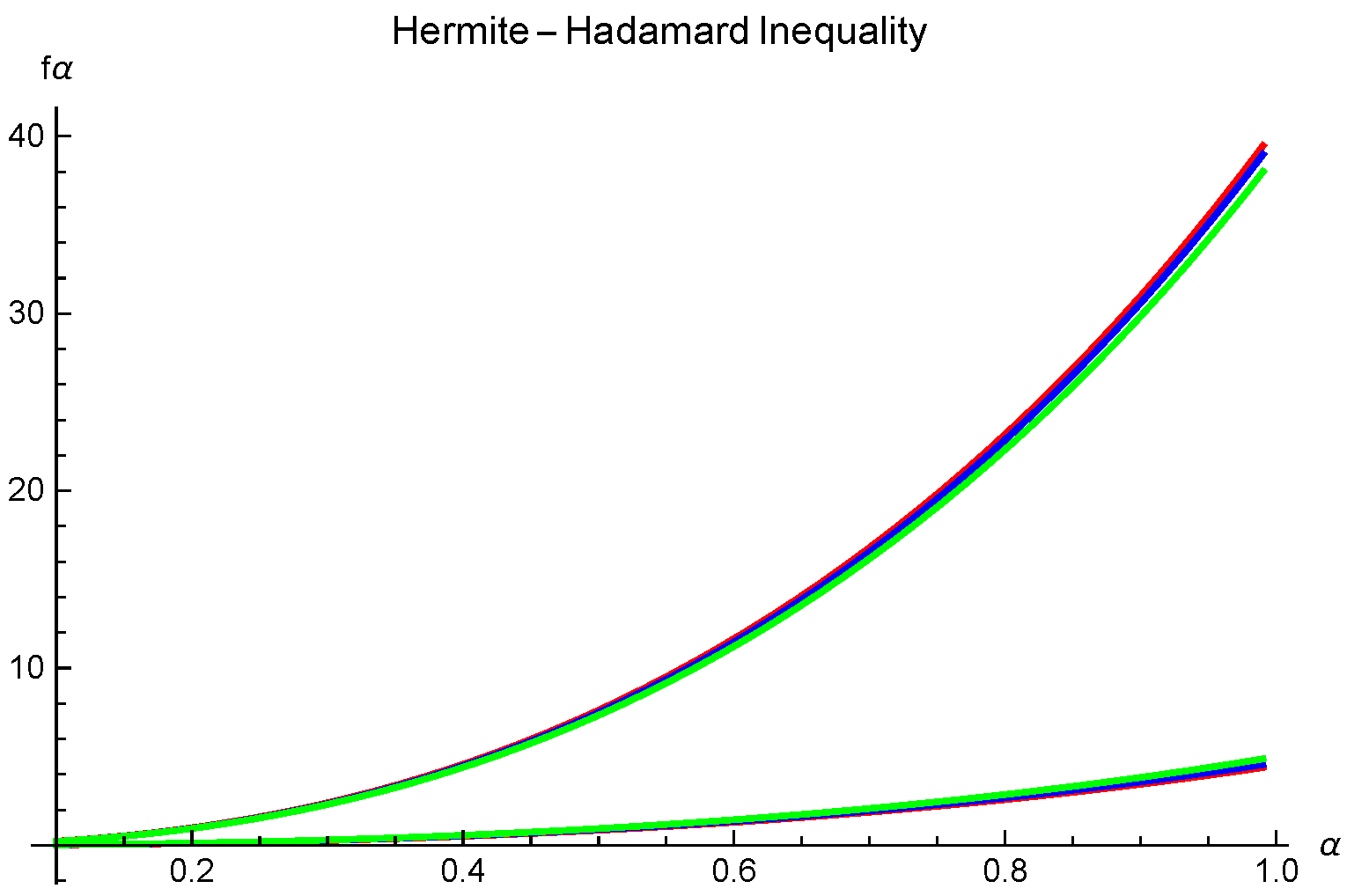
Example 1. Assume that all the assumptions of Theorem 3 are fulfilled; we take with , and with , we have For graphical visualization, we vary
(see
Figure 1).
Now, we provide the generalized fractional version of the Fejer-type HH’s-type inequality.
Theorem 4. Let be a I.V. pre-invex function with and be a continuous function; then, we have and . Proof. Since
is a
I.V. pre-invex function, for
, we have
Substituting
and
in the above inequality, multiplying both sides by
, we have
Now, we use fact that
=
Multiplying both sides by
and then adding
+
to both sides, we obtain
Multiplying both sides by
and then adding
to both sides, we acquire
To prove our second inequality, we add (
12) and (
13), multiplying both sides by
and integrating with respect to
on
; then, we have
Multiplying both sides by and then adding + to both sides, we obtain our required second inclusion. □
Now, we deliver several consequences of Theorem 4.
If we choose
in Theorem 4, we have
where
and
.
If we choose
and
in Theorem 4, then
where
and
.
If we choose
in Theorem 4, then
where
and
.
If we choose
and
in Theorem 4, then
where
and
.
If we choose
and
in Theorem 4, then
where
,
and
.
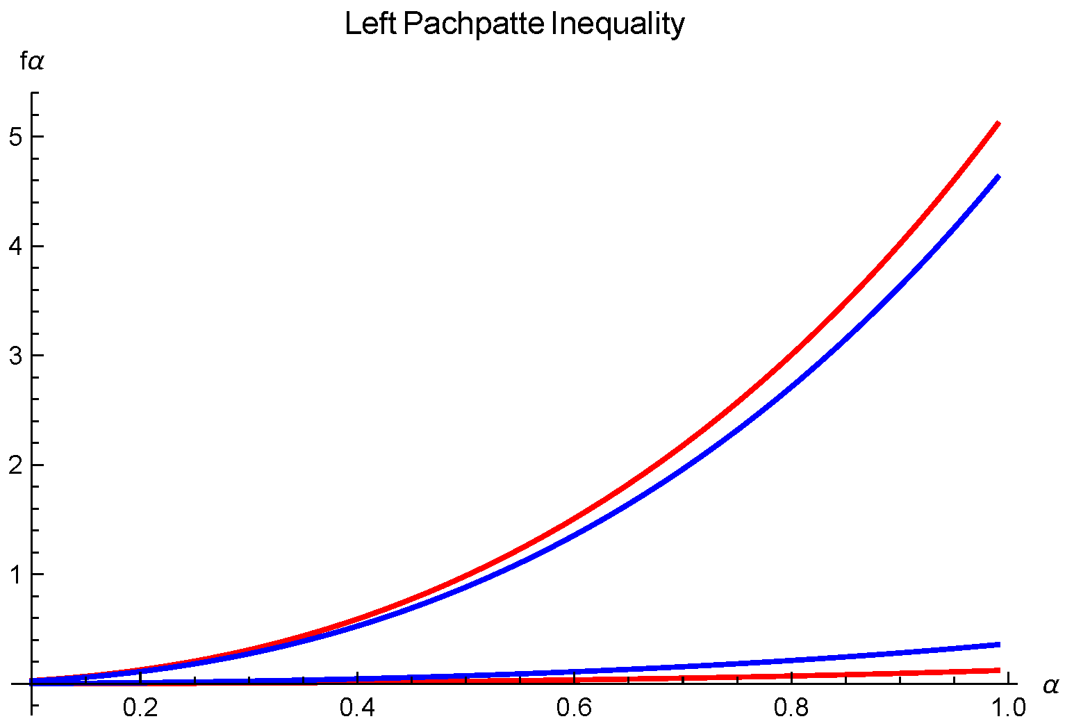
Example 2. Assume that all the assumptions of Theorem 4 are fulfilled. If we take , where with , , and and symmetric function with respect to such that and are defined as:For a graphical visualization, we vary (see Figure 2). Theorem 5. Let be I.V. pre-invex functions with and be a continuous function; then,whereand , . Proof. Since
and
are
I.V. pre-invex functions, then
Multiplying (
19) and (
20), we have
By adding (
21) and (
22), multiplying both sides by
and integrating with respect to
on
, then we have
Multiplying both sides by
and then adding
+
to both sides, we obtain
This completes the proof. □
Now, we extract a few important inclusions from Theorem 5 for the product of different kinds of convex functions.
If we choose
in Theorem 5, then
If we choose
and
in Theorem 5, then
If we choose
in Theorem 5, then
If we choose
and
in Theorem 5, then
If we choose
and
in Theorem 5, then
where
.
Example 3. Assume that all the assumptions of Theorem 5 are fulfilled. If we take where and with , and , then Theorem 6. Let be I.V. pre-invex functions with and be a continuous function; then,where and are given by (17) and (18), respectively. Proof. Since
and
are I.V.
pre-invex functions, then we have
Multiplying the proceeding inequality by
and integrating with respect to
on
, we have
Applying the definition of interval-valued convexity, we acquire
Adding
to both sides, we obtain
Comparing (
15)–(
26), we obtain our required result. □
Now, we extract a few important inclusions from Theorem 6, for the product of different kinds of convex functions.
If we choose
in Theorem 6, then
where
and
are given by (
17) and (
18), respectively.
If we choose
and
in Theorem 6, then
where
and
are given by (
17) and
, respectively.
If we choose
and
in Theorem 6, then
where
and
are given by (
17) and (
18), respectively.
If we choose
and
in Theorem 6, then
where
,
and
are given by (
17) and (
18), respectively.
Example 4. Assume that all the assumptions of Theorem 6 are fulfilled. If we take where and with , and , then 

