Adaptive Control Design for Euler–Lagrange Systems Using Fixed-Time Fractional Integral Sliding Mode Scheme

Abstract

This paper presents an adaptive fixed-time fractional integral control for externally disturbed Euler–Lagrange systems. In the first step of the control design, the approach of fractional-order fixed-time integral nonsingular terminal sliding mode control (FoIFxTSM) is introduced. This scheme combines the benefits of fractional calculus with integral sliding mode control, resulting in fast convergence, smooth nonsingular control inputs, and fixed-time stability. By integrating an adaptive scheme, the proposed method is used to control the dynamical system in the presence of uncertainty and external perturbations. The findings of the fixed-time stability using Lyapunov analyses are provided for the closed-loop system. The simulation results are compared with the adaptive fractional-order sliding mode control scheme, and they show the better tracking and convergence performance of the proposed method.

1. Introduction

The Euler–Lagrange equation, which describes the dynamics of a broad class of engineering systems, is applied to the study and modeling of nonlinear systems. In recent years, there has been an increased level of interest in the study of Euler–Lagrange systems. Generally, Euler–Lagrange systems are representations of a variety of real-world practical systems, such as mobile robot platforms [1,2], helicopter [3,4], oscillatory systems [5], aircraft [6,7], pneumatic muscles [8], bipedal robots [9], robotic manipulators [10], cranes [11], spacecraft [12], etc. These technologies have enormous potential uses in a variety of fields, including military operations, the automation industry, surveillance, and space exploration. Since this is a nonlinear system with a significant degree of mechanical instability, it necessitates a high level of control and stability. As a result, it must be carefully controlled. Several workable strategies have been presented for uncertain Euler–Lagrange systems that are influenced by environmental disturbances. Therefore, in order to ensure that the system continues to perform its intended functions in spite of the existence of unknown dynamics, a robust adaptive control mechanism is constructed. One of the benefits of the methodology that lies behind robust and adaptive schemes is that the control system becomes robust and updates control parameters according to the current situation to ensure appropriate degree of stability [13].

Intensive research attention focuses on the control of Euler–Lagrange systems [1]. Various methods in the literature have been proposed to handle the tracking problem, such as disturbance observer [11], sliding-mode approach [12], expanded proportional–integral controller [14], and adaptive fuzzy control [15]. Adaptive control, a well-recognized and widely used control method, is becoming increasingly prevalent in control engineering applications. It exhibits exceptional potential for adjusting to different environments under unknown and uncertain dynamics, hence enhancing the tracking performance of closed-loop systems [16]. Performance degradation and instability may result from parametric and non-parametric uncertainties; therefore, further developments in control theory are introduced to use adaptive control to deal with unknown uncertainties [13]. Moreover, sliding mode control (SMC) is a type of nonlinear robust control strategy. It is able to successfully control uncertain nonlinear systems with bounded disturbances and minimal sensitivity to changes in the system’s characteristics. Various advancements have been made for SMC, such as terminal SMC (TSMC), nonsingular TSMC, fast TSMC, integral TSMC, and fast nonsingular TSMC [17,18,19,20]. Furthermore, fractional-order (Fo) control has been incorporated with SMC to improve the performance of the controller [21,22,23]. Fractional-order control, which has been in use for the last three centuries and is concerned with derivatives and integrals of a non-integer order, was recently rediscovered by scientists and engineers and is being put to use in a variety of different fields [24,25,26,27,28].

Setting up a nonlinear system with appropriate initial conditions has a substantial influence on how long it takes to converge in finite time, and this time changes as the nonlinear system’s initial conditions change. A fixed-time control scheme is consequently a substitute that is applied to exactly calculate the convergence time and does not rely on the initial values [29,30,31]. Various fractional-order TSMC (FoSMC) schemes have been designed and applied to several Euler–Lagrange systems. In [32,33], a finite-time linear–quadratic regulator with the FoSMC method and a fixed-time nonsingular FoSMC scheme have been developed, respectively, for the known dynamics of nonlinear robotic systems. To deal with unknown dynamics, there are several adaptive FoSMC strategies that may be used with Euler–Lagrange systems, and these techniques take into consideration the presence of unknown uncertainties and disturbances as well. In [34], adaptive finite-time FoSMC scheme is designed for robotic manipulators, which provides fast finite-time convergence; however, finite-time control depends on the initial values of states, and its convergence varies with the initial positions. A robust adaptive finite-time FoSMC using time delay control was constructed for the nonlinear robotic system [14]. This method provides robust performance; however, the constant delay inserted may cause instability in the system. Moreover, using an adaptive controller to estimate the behaviors of the unknowable dynamics contained within the model, a finite-time FoSMC was used to provide robustness for a nonlinear robot, and this adaptive scheme was designed using a radial basis function neural network [35]. However, the disadvantage of the neural network schemes is that they require heavy online calculation in the training of unknown system parameters and controller gains.

Using a finite-time sliding mode approach to estimate the bounded unknown and uncertain dynamics, each of the aforementioned papers placed a strong emphasis on the adaptive approach. Therefore, the main advantage of the proposed FoIFxTSM control is that it eliminates the possibility of nonsingularity, makes the system resilient against unknown dynamics and external disturbances, and ensures that the convergence rate is independent of the initial conditions. According to the study, adaptive FoIFxTSM control has not been investigated, and only a small number of studies have given adaptive fractional-order FxTSM control. So, this research examines the fixed-time scheme for externally perturbed Euler–Lagrange systems. More specifically, this research explores the effects of system dynamics that are unknown. Hence, an investigation is carried out to design the adaptive fractional-order integral nonsingular TSMC (AFoIFxTSM) for the uncertain Euler–Lagrange system subject to unknown external disturbances.

The significant contributions provided by this study are described as follows:

• Based on the characteristics of fixed-time integral nonsingular TSMC, a sliding surface is designed that provides excellent tracking performance, minimal chattering in control inputs, nonsingularity, and a fast rate of convergence.
• The fractional-order technique is used to enhance the performance of the closed system.
• Adaptive control using FoIFxTSM is presented for the Euler–Lagrange system to provide robust and sustainable performance by mitigating the effects of unknown uncertainties in the system’s dynamics.
• The Lyapunov synthesis is employed to investigate the fixed-time stability of the proposed system, and it also provides fixed-time formulations.

The remaining sections of this work are organized in the following way: The preliminaries and notations are given in Section 2. The system’s modeling, control scheme, and stability are all covered in Section 3. The adaptive control approach and the proof of stability are given in Section 4. The numerical results and discussions of the suggested technique are shown in Section 5. Section 6 contains the conclusion.

2. Preliminaries and Notations

Definition 1. 

The definition given by Riemann–Liouville (RL) is widely used in fractional calculus [36,37]. The derivative of the ${\beta }_{th}$-order as a function of time, $f\left(t\right)$, and the constant a can be calculated using the following equation, which also provides the RL fractional integral:

$${}_a{\mathfrak{I}}_t^{\beta }f\left(t\right)=\frac{1}{\Gamma \left(\beta \right)}{\int }_a^t\frac{f\left(\tau \right)}{{(t-\tau )}^{1-\beta }}d\tau$$

(1)

$${}_a{\mathfrak{D}}_t^{\beta }f\left(t\right)=\frac{d^{\beta }f\left(t\right)}{d{t}^{\beta }}=\frac{1}{\Gamma (1-\beta )}\frac{d}{dt}{\int }_a^t\frac{f\left(\tau \right)}{{(t-\tau )}^{\beta }}d\tau$$

(2)

where $m-1<\beta <m$, $m\in \mathbb{N}$. $\Gamma \left(\beta \right)$ is the Euler gamma function, defined as

$$\Gamma \left(\beta \right)={\int }_0^{\infty }{e}^{-t}{t}^{\beta -1}dt$$

The fractional integral and derivative in the above equations are represented by the symbols $\mathfrak{I}$ and $\mathfrak{D}$, respectively.

Lemma 1 

([38]). Consider the following nonlinear model:

$$\dot{x}\left(t\right)=f(t,x),x\left(0\right)=x_0$$

(3)

where the function $f(t,x)$ is continuous. The Lyapunov function $V\left(x\right)$ fulfills the following requirements for fixed-time stability with fast convergence:

i. 

$V\left(x\right)=0\iff x=0$

ii. 

$\dot{V}\left(x\right)\le -{\phi }_1{V}^{{\varphi }_1}\left(x\right)-{\phi }_{2}V{\left(x\right)}^{{\varphi }_2}$

with ${\phi }_1,{\phi }_2>0,0<{\varphi }_1<1and{\varphi }_2>1$. After that, the system is said to be stable in fixed time, and the time required for convergence is upper-bounded as

$$T\le \frac{1}{{\phi }_1(1-{\varphi }_1)}+\frac{1}{{\phi }_2({\varphi }_2-1)}$$

(4)

Notations.

The power of vectors is defined as

$${\left[\left[x\right]\right]}^y={\left[{\left|x_1\right|}^{y}sign\left(x_1\right),{\left|x_2\right|}^{y}sign\left(x_2\right),\dots ,{\left|x_n\right|}^{y}sign\left(x_n\right)\right]}^T$$

and

$${\left|x\right|}^{y-1}=diag\left({\left|x_1\right|}^{y-1},{\left|x_2\right|}^{y-1},\cdots ,{\left|x_n\right|}^{y-1}\right)$$

where x is considered as a variable and y is a constant.

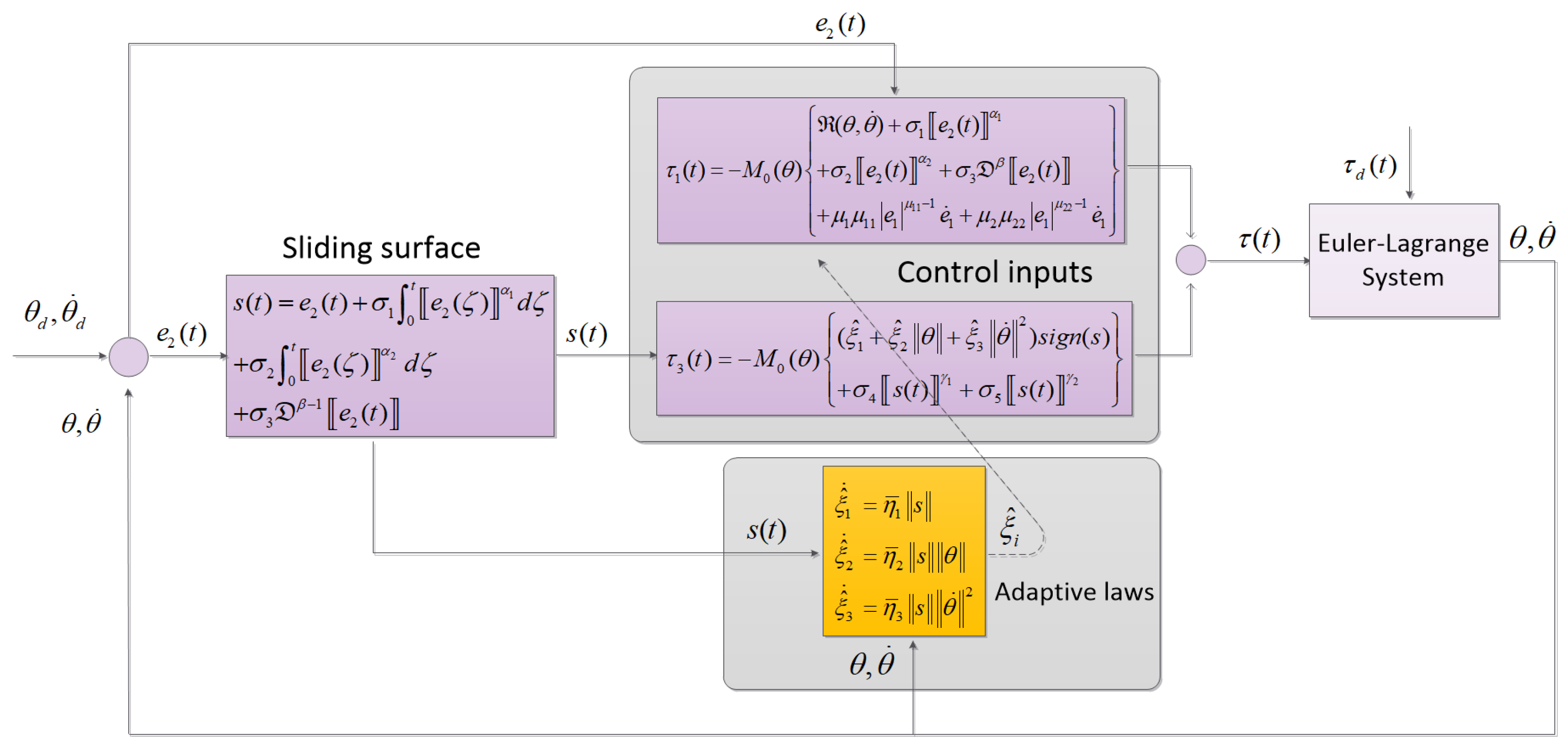
3. Designing Adaptive Fixed-Time Fractional Integral SMC Scheme

This section starts with an explanation of the dynamics of the Euler–Lagrange system. It then investigates a fixed-time fractional-order integral nonsingular sliding surface and concludes with the design of the proposed scheme.

The dynamic equation of an Euler–Lagrange system is given by [14]

$$M\left(\theta \right)\ddot{\theta }+C(\theta ,\dot{\theta })\dot{\theta }+G\left(\theta \right)=\tau \left(t\right)+{\tau }_d\left(t\right)$$

(5)

where $M\left(\theta \right)=M_0\left(\theta \right)+\hat{M}\left(\theta \right),C(\theta ,\dot{\theta })=C_0(\theta ,\dot{\theta })+\widehat{C}(\theta ,\dot{\theta })$ and $G\left(\theta \right)=G_0\left(\theta \right)+\hat{G}\left(\theta \right)$. Moreover, $M_0$, $C_0$, $G_0$ and $\hat{M}$, $\hat{C}$, $\hat{G}$ are nominal and uncertain parameters, respectively. $\theta \in \mathbb{R}{}^n$ denotes the angular position, $\dot{\theta }\in \mathbb{R}{}^n$ represents the angular velocity, and $\ddot{\theta }\in \mathbb{R}{}^n$ is the angular acceleration. $M\left(\theta \right)\in \mathbb{R}{}^{n\times n}$ is the inertia matrix and meets the condition that $M_1\left(M\left(\theta \right)\right)\le ∥M\left(\theta \right)∥\le M_2\left(M\left(\theta \right)\right)$, where $M_1>0$ and $M_2>0$ are respectively the minimum and maximum eigenvalues of $M\left(\theta \right)$, $C(\theta ,\dot{\theta })\in \mathbb{R}{}^{n\times n}$ is the coriolis and centripetal force, $G\left(\theta \right)\in \mathbb{R}{}^n$ is the gravitational force, ${\tau }_d\left(t\right)\in \mathbb{R}{}^n$ represents the external disturbances, and $\tau \left(t\right)\in \mathbb{R}{}^n$ is the control input torque.

Rewriting the dynamic Equation (5) yields

$$\ddot{\theta }=M_0^{-1}\left(\theta \right)\tau -M_0^{-1}\left(\theta \right)[C_0(\theta ,\dot{\theta })\dot{\theta }+G_0\left(\theta \right)]+\mathfrak{U}(\theta ,\dot{\theta },\ddot{\theta },{\tau }_d)$$

(6)

where $\mathfrak{U}(\theta ,\dot{\theta },\ddot{\theta },{\tau }_d)=M_0^{-1}\left(\theta \right)\left[{\tau }_d\left(t\right)-\widehat{M}\left(\theta \right)\ddot{\theta }-\widehat{C}(\theta ,\dot{\theta })\dot{\theta }-\widehat{G}\left(\theta \right)\right]$ represents the uncertainties and external disturbances in the Euler–Lagrange system.

In order to derive the tracking error, we use (6) as follows:

$${\ddot{e}}_1=M_0^{-1}\left(\theta \right)\tau +\mathfrak{N}(\theta ,\dot{\theta })+\mathfrak{U}(\theta ,\dot{\theta },\ddot{\theta },{\tau }_d)$$

(7)

where $\mathfrak{N}(\theta ,\dot{\theta })=-M_0^{-1}\left(\theta \right)[C_0(\theta ,\dot{\theta })\dot{\theta }+G_0\left(\theta \right)]-{\ddot{\theta }}_d$ is the nominal dynamics and ${\theta }_d$ is the joint’s desired angular position. The tracking error is then defined as $e_1=\theta -{\theta }_d$.

Assumption A1. 

The expression (8), which can be seen below, provides the bounded condition of uncertain dynamics [39]

$$∥\mathfrak{U}(\theta ,\dot{\theta },\ddot{\theta },{\tau }_d)∥\le {\xi }_1+{\xi }_2∥\theta ∥+{\xi }_3{∥\dot{\theta }∥}^2$$

(8)

where ${\xi }_1$, ${\xi }_2$ and ${\xi }_3$ are unknown bound constants of uncertainties and disturbances.

3.1. Fractional Integral Sliding Manifold

In this subsection, the fixed-time integral fractional-order sliding surface is designed, which gives the nonlinear system’s accurate and precise tracking performance in fixed time:

$$s\left(t\right)=e_2\left(t\right)+{\sigma }_1{\int }_0^t{\left[\left[e_2\left(\zeta \right)\right]\right]}^{{\alpha }_1}d\zeta +{\sigma }_2{\int }_0^t{\left[\left[e_2\left(\zeta \right)\right]\right]}^{{\alpha }_2}d\zeta +{\sigma }_3{\mathfrak{D}}^{\beta -1}\left[\left[e_2\left(t\right)\right]\right]$$

(9)

where $\begin{array}{c}{e}_2\left(t\right)={\dot{e}}_1\left(t\right)+{\mu }_1{\left[\left[e_1\left(t\right)\right]\right]}^{{\mu }_{11}}+{\mu }_2{\left[\left[e_1\left(t\right)\right]\right]}^{{\mu }_{22}},\hfill \end{array}$$s\left(t\right)\in \mathbb{R}{}^n$ represents the sliding surface, ${\sigma }_1>0$, ${\sigma }_2>0$, ${\sigma }_3>0$, ${\mu }_1>0$ and ${\mu }_2>0$. Moreover, exponential values are $0<{\alpha }_1<1$, $1<{\alpha }_2$, $0<{\mu }_{11}<1$, $1<{\mu }_{22}$ and the fractional order has $0<\beta <1$:

$$\begin{array}{c}\dot{s}\left(t\right)={\dot{e}}_2\left(t\right)+{\sigma }_1{\left[\left[e_2\left(t\right)\right]\right]}^{{\alpha }_1}+{\sigma }_2{\left[\left[e_2\left(t\right)\right]\right]}^{{\alpha }_2}+{\sigma }_3{\mathfrak{D}}^{\beta }\left[\left[e_2\left(t\right)\right]\right]\hfill \\ ={\ddot{e}}_1\left(t\right)+{\mu }_1{\mu }_{11}{\left|e_1\left(t\right)\right|}^{{\mu }_{11}-1}{\dot{e}}_1\left(t\right)+{\mu }_2{\mu }_{22}{\left|e_1\left(t\right)\right|}^{{\mu }_{22}-1}{\dot{e}}_1\left(t\right)\hfill \\ +{\sigma }_1{\left[\left[e_2\left(t\right)\right]\right]}^{{\alpha }_1}+{\sigma }_2{\left[\left[e_2\left(t\right)\right]\right]}^{{\alpha }_2}+{\sigma }_3{\mathfrak{D}}^{\beta }\left[\left[e_2\left(t\right)\right]\right]\hfill \end{array}$$

(10)

with ${\left|e_1\left(t\right)\right|}^{{\mu }_{11}-1}=0$ if $e_1\left(t\right)=0$.

Substituting (7) into (10) yields

$$\begin{array}{c}\dot{s}\left(t\right)=M_0^{-1}\left(\theta \right)\tau +\mathfrak{N}(\theta ,\dot{\theta })+\mathfrak{U}(\theta ,\dot{\theta },\ddot{\theta },{\tau }_d)\hfill \\ +{\mu }_1{\mu }_{11}{\left|e_1\left(t\right)\right|}^{{\mu }_{11}-1}{\dot{e}}_1\left(t\right)+{\mu }_2{\mu }_{22}{\left|e_1\left(t\right)\right|}^{{\mu }_{22}-1}{\dot{e}}_1\left(t\right)\hfill \\ +{\sigma }_1{\left[\left[e_2\left(t\right)\right]\right]}^{{\alpha }_1}+{\sigma }_2{\left[\left[e_2\left(t\right)\right]\right]}^{{\alpha }_2}+{\sigma }_3{\mathfrak{D}}^{\beta }\left[\left[e_2\left(t\right)\right]\right]\hfill \end{array}$$

(11)

Now that the sliding manifold is finalized, the proposed FoIFxTSM method for uncertain Euler–Lagrange systems is designed so that the goal of achieving robust performance with external disturbances can be reached.

3.2. FoIFxTSM Control Design

The FoIFxTSM control law can be designed as follows, with the objective of controlling the nonlinear Euler–Lagrange system under known bounded uncertainties and disturbances:

$$\tau \left(t\right)={\tau }_1\left(t\right)+{\tau }_2\left(t\right)$$

(12)

where ${\tau }_1\left(t\right)$ and ${\tau }_2\left(t\right)$ are used for control, with the nominal and uncertain system. The proposed ${\tau }_1\left(t\right)$ and ${\tau }_2\left(t\right)$ are given as

$$\begin{array}{c}\hfill {\tau }_1\left(t\right)=-M_0^{}\left(\theta \right)\left\{\begin{array}{c}\begin{array}{c}\mathfrak{N}(\theta ,\dot{\theta })+{\sigma }_1{\left[\left[e_2\left(t\right)\right]\right]}^{{\alpha }_1}\hfill \\ +{\sigma }_2{\left[\left[e_2\left(t\right)\right]\right]}^{{\alpha }_2}+{\sigma }_3{\mathfrak{D}}^{\beta }\left[\left[e_2\left(t\right)\right]\right]\hfill \\ +{\mu }_1{\mu }_{11}{\left|e_1\left(t\right)\right|}^{{\mu }_{11}-1}{\dot{e}}_1\left(t\right)\hfill \\ +{\mu }_2{\mu }_{22}{\left|e_1\left(t\right)\right|}^{{\mu }_{22}-1}{\dot{e}}_1\left(t\right)\hfill \end{array}\hfill \end{array}\right\}\end{array}$$

(13)

$$\begin{array}{c}\hfill {\tau }_2\left(t\right)=-M_0^{}\left(\theta \right)\left\{\begin{array}{c}({\xi }_1+{\xi }_2∥\theta ∥+{\xi }_3{∥\dot{\theta }∥}^2)sign\left(s\right)\hfill \\ +{\sigma }_4{\left[\left[s\left(t\right)\right]\right]}^{{\gamma }_1}+{\sigma }_5{\left[\left[s\left(t\right)\right]\right]}^{{\gamma }_2}\hfill \end{array}\right\}\end{array}$$

(14)

where ${\sigma }_4>0$ and ${\sigma }_5>0$ are constants. ${\gamma }_1$ and ${\gamma }_2$ have ranges as $0<{\gamma }_1<1$ and $1<{\gamma }_2$, respectively.

3.3. Stability Analysis

Within this subsection, to figure out the stability of a closed-loop system, the Lyapunov analysis will be used.

Theorem 1. 

We take into account the Euler–Lagrange system that is described in (5), the sliding manifold that is suggested in (9) and the FoIFxTSM controller that is designed in (12) for the uncertain dynamics intended angular position in a fixed amount of time to converge under Assumption 1 (8).

Proof. 

The following Lyapunov functional candidate is given as

$$V_1=\frac{1}{2}\sum _{i=1}^n{s}_i^2\left(t\right)$$

(15)

Then, ${\dot{V}}_1\left(t\right)$ is derived as

$${\dot{V}}_1=\sum _{i=1}^n{s}_i^{}\left(t\right){\dot{s}}_i^{}\left(t\right)$$

(16)

From (10), $\dot{s}\left(t\right)$ is substituted into the Equation (16), and we obtain

$${\dot{V}}_1=\sum _{i=1}^n{s}_i^{}\left(t\right)\left[\begin{array}{c}{\dot{e}}_{2i}\left(t\right)+{\sigma }_1{\left[\left[e_{2i}\left(t\right)\right]\right]}^{{\alpha }_1}+{\sigma }_2{\left[\left[e_{2i}\left(t\right)\right]\right]}^{{\alpha }_2}\hfill \\ +{\sigma }_3{\mathfrak{D}}^{\beta }\left[\left[e_{2i}\left(t\right)\right]\right]\hfill \end{array}\right]$$

(17)

The substitution of ${\ddot{e}}_1\left(t\right)$ derived from (7) into (17) yields

$${\dot{V}}_1=\sum _{i=1}^n{s}_i^{}\left(t\right)\left\{\begin{array}{c}{M}_{0i}^{-1}\left(\theta \right){\tau }_i+{\mathfrak{N}}_{\mathfrak{i}}(\theta ,\dot{\theta })+{\mathfrak{U}}_{\mathfrak{i}}(\theta ,\dot{\theta },\ddot{\theta },{\tau }_d)\hfill \\ +{\sigma }_1{\left[\left[e_{2i}\left(t\right)\right]\right]}^{{\alpha }_1}+{\sigma }_2{\left[\left[e_{2i}\left(t\right)\right]\right]}^{{\alpha }_2}\hfill \\ +{\sigma }_3{\mathfrak{D}}^{\beta }\left[\left[e_{2i}\left(t\right)\right]\right]\hfill \\ +{\mu }_1{\mu }_{11}{\left|e_{1i}\left(t\right)\right|}^{{\mu }_{11}-1}{\dot{e}}_{1i}\left(t\right)\hfill \\ +{\mu }_2{\mu }_{22}{\left|e_{1i}\left(t\right)\right|}^{{\mu }_{22}-1}{\dot{e}}_{1i}\left(t\right)\hfill \end{array}\right\}$$

(18)

With the substitution of $\tau \left(t\right)$ obtained from (12) into (18), we have

$${\dot{V}}_1=\sum _{i=1}^n{s}_i^{}\left(t\right)\left[\begin{array}{c}-\left\{\begin{array}{c}\begin{array}{c}({\xi }_1+{\xi }_2∥\theta ∥+{\xi }_3{∥\dot{\theta }∥}^2)sign\left(s_i\right)\hfill \\ +{\mathfrak{N}}_{\mathfrak{i}}(\theta ,\dot{\theta })+{\sigma }_3{\mathfrak{D}}^{\beta }\left[\left[e_{2i}\left(t\right)\right]\right]\hfill \end{array}\hfill \\ +{\sigma }_1{\left[\left[e_{2i}\left(t\right)\right]\right]}^{{\alpha }_1}+{\sigma }_2{\left[\left[e_{2i}\left(t\right)\right]\right]}^{{\alpha }_2}\hfill \\ +{\sigma }_4{\left[\left[s_i\left(t\right)\right]\right]}^{{\gamma }_1}+{\sigma }_5{\left[\left[s_i\left(t\right)\right]\right]}^{{\gamma }_2}\hfill \\ +{\mu }_1{\mu }_{11}{\left|e_{1i}\left(t\right)\right|}^{{\mu }_{11}-1}{\dot{e}}_{1i}\left(t\right)\hfill \\ +{\mu }_2{\mu }_{22}{\left|e_{1i}\left(t\right)\right|}^{{\mu }_{22}-1}{\dot{e}}_{1i}\left(t\right)\hfill \end{array}\right\}\hfill \\ \begin{array}{c}+{\mathfrak{N}}_{\mathfrak{i}}(\theta ,\dot{\theta })+{\mathfrak{U}}_{\mathfrak{i}}(\theta ,\dot{\theta },\ddot{\theta },{\tau }_d)\hfill \\ +{\sigma }_1{\left[\left[e_{2i}\left(t\right)\right]\right]}^{{\alpha }_1}+{\sigma }_2{\left[\left[e_{2i}\left(t\right)\right]\right]}^{{\alpha }_2}\hfill \\ +{\sigma }_3{\mathfrak{D}}^{\beta }\left[\left[e_{2i}\left(t\right)\right]\right]\hfill \\ +{\mu }_1{\mu }_{11}{\left|e_{1i}\left(t\right)\right|}^{{\mu }_{11}-1}{\dot{e}}_{1i}\left(t\right)\hfill \\ +{\mu }_2{\mu }_{22}{\left|e_{1i}\left(t\right)\right|}^{{\mu }_{22}-1}{\dot{e}}_{1i}\left(t\right)\hfill \end{array}\hfill \end{array}\right]$$

(19)

With the simplification of (19), we obtain

$${\dot{V}}_1=\sum _{i=1}^n{s}_i^{}\left(t\right)\left[\begin{array}{c}-\left\{\begin{array}{c}({\xi }_1+{\xi }_2∥\theta ∥+{\xi }_3{∥\dot{\theta }∥}^2)sign\left(s_i\right)\hfill \\ +{\sigma }_4{\left[\left[s_i\left(t\right)\right]\right]}^{{\gamma }_1}+{\sigma }_5{\left[\left[s_i\left(t\right)\right]\right]}^{{\gamma }_2}\hfill \end{array}\right\}\hfill \\ +{\mathfrak{U}}_{\mathfrak{i}}(\theta ,\dot{\theta },\ddot{\theta },{\tau }_d)\hfill \end{array}\right]$$

(20)

Based on Assumption 1, we have

$$\begin{array}{c}{\dot{V}}_1\le -{\displaystyle \sum _{i=1}^n}{s}_i^{}\left(t\right)\left[{\sigma }_4{\left[\left[s_i\left(t\right)\right]\right]}^{{\gamma }_1}+{\sigma }_5{\left[\left[s_i\left(t\right)\right]\right]}^{{\gamma }_2}\right]\hfill \\ \le -{\sigma }_4{\displaystyle \sum _{i=1}^n}{\left|s_i\left(t\right)\right|}^{{\gamma }_1+1}-{\sigma }_5{\displaystyle \sum _{i=1}^n}{\left|s_i\left(t\right)\right|}^{{\gamma }_2+1}\hfill \\ \le -{\sigma }_4{\displaystyle \sum _{i=1}^n}{\left({\left|s_i^{}\left(t\right)\right|}^2\right)}^{\frac{{\gamma }_1+1}{2}}-{\sigma }_5{\displaystyle \sum _{i=1}^n}{\left({\left|s_i^{}\left(t\right)\right|}^2\right)}^{\frac{{\gamma }_2+1}{2}}\hfill \end{array}$$

(21)

In accordance with the inequality presented in [40], we obtain

$$\begin{array}{c}{\dot{V}}_1\le -{\sigma }_4{\left({\displaystyle \sum _{i=1}^n}{\left|s_i^{}\left(t\right)\right|}^2\right)}^{\frac{{\gamma }_1+1}{2}}-{\sigma }_5{n}^{\frac{1-{\gamma }_2}{2}}{\left({\displaystyle \sum _{i=1}^n}{\left|s_i^{}\left(t\right)\right|}^2\right)}^{\frac{{\gamma }_2+1}{2}}\hfill \\ \le -{\sigma }_4{\left(2V_1\right)}^{\frac{{\gamma }_1+1}{2}}-{\sigma }_5{n}^{\frac{1-{\gamma }_2}{2}}{\left(2V_1\right)}^{\frac{{\gamma }_2+1}{2}}\hfill \\ \le -2^{\frac{{\gamma }_1+1}{2}}{\sigma }_4{V_1}^{\frac{{\gamma }_1+1}{2}}-2^{\frac{{\gamma }_2+1}{2}}{\sigma }_5{n}^{\frac{1-{\gamma }_2}{2}}{V_1}^{\frac{{\gamma }_2+1}{2}}\hfill \end{array}$$

(22)

Consequently, in a fixed amount of time, the system’s states reach $s\left(t\right)$. Based on Lemma 1, the fixed settling time is formulated as

$$T_1=\frac{1}{2^{\frac{{\gamma }_1+1}{2}}{\sigma }_4\left(1-\frac{{\gamma }_1+1}{2}\right)}+\frac{1}{2^{\frac{{\gamma }_2+1}{2}}{n}^{\frac{1-{\gamma }_2}{2}}{\sigma }_5\left(\frac{{\gamma }_2+1}{2}-1\right)}$$

(23)

The total settling can be obtained using the relation $T_{s1}=T_1+T_2+T_3$, where $T_2$ can be formulated when $e_2\left(t\right)=0$; therefore, it is written as ${\dot{e}}_1\left(t\right)=-{\mu }_1{\left[\left[e_1\left(t\right)\right]\right]}^{{\mu }_{11}}-{\mu }_2{\left[\left[e_1\left(t\right)\right]\right]}^{{\mu }_{22}}$. Furthermore, $T_3$ can be computed when the sliding surface $s\left(t\right)=0$. Therefore, using (9), the following expression is obtained:

$${\dot{e}}_2\left(t\right)=-{\sigma }_1{\left[\left[e_2\left(t\right)\right]\right]}^{{\alpha }_1}-{\sigma }_2{\left[\left[e_2\left(t\right)\right]\right]}^{{\alpha }_2}-{\sigma }_3{\mathfrak{D}}^{\beta }\left[\left[e_2\left(t\right)\right]\right]$$

(24)

It can be deduced from Lemma 1 that the tracking errors are stable in fixed time. Thus, the constant $T_2$ can be formulated so that the error eventually converges to zero for $T_{s1}$. □

4. Adaptive FoIFxTSM Control Design

The following equations provide a description of how the control input is designed, making use of an adaptive scheme to tackle the unknown and uncertain dynamics:

$$\tau \left(t\right)={\tau }_1\left(t\right)+{\tau }_3\left(t\right)$$

(25)

where ${\tau }_1\left(t\right)$ is same as (13) and

$${\tau }_3\left(t\right)=-M_0^{}\left(\theta \right)\left\{\begin{array}{c}({\widehat{\xi }}_1+{\widehat{\xi }}_2∥\theta ∥+{\widehat{\xi }}_3{∥\dot{\theta }∥}^2)sign\left(s\right)\\ +{\sigma }_4{\left[\left[s\left(t\right)\right]\right]}^{{\gamma }_1}+{\sigma }_5{\left[\left[s\left(t\right)\right]\right]}^{{\gamma }_2}\end{array}\right\}$$

(26)

whereas ${\hat{\xi }}_1$, ${\hat{\xi }}_2$ and ${\hat{\xi }}_3$ denote the estimation variable of ${\xi }_1,{\xi }_2$ and ${\xi }_3$, respectively.

The following adaptive laws are presented as potential solutions to deal with the unknown dynamics

$${\dot{\hat{\xi }}}_1^{}={\overline{\eta }}_1∥s∥,{\dot{\hat{\xi }}}_2^{}={\overline{\eta }}_2∥s∥∥\theta ∥,{\dot{\hat{\xi }}}_3^{}={\overline{\eta }}_3∥s∥{∥\dot{\theta }∥}^2$$

(27)

where ${\overline{\eta }}_1,{\overline{\eta }}_2$and${\overline{\eta }}_3>0$, and the proposed model is given in Figure 1.

The problem of compensating for the unknown dynamics can be solved using (25). As a result, the AFoIFxTSM approach ultimately obtains the tracking performance when an uncertain dynamical system is subject to unknown disturbances.

Theorem 2. 

We consider the Euler–Lagrange system (5) and the degree to which it is susceptible to problems, including uncertainty and external disturbances. As a consequence of this, the desired states converge in a fixed time under Assumption 1 because of the proposed sliding surface (9), the designed AFoIFxTSM control (25), and adaptive control laws (27).

Proof. 

The selected Lyapunov function is as follows:

$$V_2=\frac{1}{2}\sum _{i=1}^n{s}_i^2\left(t\right)+\frac{1}{2{\eta }_1}{\tilde{\xi }}_1^2+\frac{1}{2{\eta }_2}{\tilde{\xi }}_2^2+\frac{1}{2{\eta }_3}{\tilde{\xi }}_3^2$$

(28)

where ${\tilde{\xi }}_1={\widehat{\xi }}_1-{\xi }_1,{\tilde{\xi }}_2={\widehat{\xi }}_2-{\xi }_2,{\tilde{\xi }}_3={\widehat{\xi }}_3-{\xi }_3$ represent the estimation errors. ${\dot{V}}_2\left(t\right)$ is given as

$${\dot{V}}_2=\sum _{i=1}^n{s}_i^{}\left(t\right){\dot{s}}_i^{}\left(t\right)+\frac{1}{{\eta }_1}{\tilde{\xi }}_1^{}{\dot{\widehat{\xi }}}_1^{}+\frac{1}{{\eta }_2}{\tilde{\xi }}_2^{}{\dot{\widehat{\xi }}}_2^{}+\frac{1}{{\eta }_3}{\tilde{\xi }}_3^{}{\dot{\widehat{\xi }}}_3^{}$$

(29)

With the substitution of $\dot{s}\left(t\right)$ derived from (10) into (29), we obtain

$$\begin{array}{c}{\dot{V}}_2={\displaystyle \sum _{i=1}^n}{s}_i^{}\left(t\right)\left\{\begin{array}{c}{M}_{0i}^{-1}\left(\theta \right){\tau }_i+{\mathfrak{N}}_{\mathfrak{i}}(\theta ,\dot{\theta })+{\mathfrak{U}}_{\mathfrak{i}}(\theta ,\dot{\theta },\ddot{\theta },{\tau }_d)\\ \begin{array}{c}+{\sigma }_1{\left[\left[e_{2i}\left(t\right)\right]\right]}^{{\alpha }_1}+{\sigma }_2{\left[\left[e_{2i}\left(t\right)\right]\right]}^{{\alpha }_2}\hfill \\ +{\sigma }_3{\mathfrak{D}}^{\beta }\left[\left[e_{2i}\left(t\right)\right]\right]\hfill \\ +{\mu }_1{\mu }_{11}{\left|e_{1i}\left(t\right)\right|}^{{\mu }_{11}-1}{\dot{e}}_{1i}\left(t\right)\hfill \\ +{\mu }_2{\mu }_{22}{\left|e_{1i}\left(t\right)\right|}^{{\mu }_{22}-1}{\dot{e}}_{1i}\left(t\right)\hfill \end{array}\end{array}\right\}\hfill \\ +\frac{1}{{\eta }_1}{\tilde{\xi }}_1^{}{\dot{\widehat{\xi }}}_1^{}+\frac{1}{{\eta }_2}{\tilde{\xi }}_2^{}{\dot{\widehat{\xi }}}_2^{}+\frac{1}{{\eta }_3}{\tilde{\xi }}_3^{}{\dot{\widehat{\xi }}}_3^{}\hfill \end{array}$$

(30)

By substituting (25) into (30), we obtain

$$\begin{array}{c}{\dot{V}}_2={\displaystyle \sum _{i=1}^n}{s}_i^{}\left(t\right)\left[\begin{array}{c}-\left\{\begin{array}{c}\begin{array}{c}({\widehat{\xi }}_1+{\widehat{\xi }}_2∥\theta ∥+{\widehat{\xi }}_3{∥\dot{\theta }∥}^2)sign\left(s_i\right)\hfill \\ +{\mathfrak{N}}_{\mathfrak{i}}(\theta ,\dot{\theta })+{\sigma }_3{\mathfrak{D}}^{\beta }\left[\left[e_{2i}\left(t\right)\right]\right]\hfill \end{array}\hfill \\ +{\sigma }_1{\left[\left[e_{2i}\left(t\right)\right]\right]}^{{\alpha }_1}+{\sigma }_2{\left[\left[e_{2i}\left(t\right)\right]\right]}^{{\alpha }_2}\hfill \\ +{\sigma }_4{\left[\left[s_i\left(t\right)\right]\right]}^{{\gamma }_1}+{\sigma }_5{\left[\left[s_i\left(t\right)\right]\right]}^{{\gamma }_2}\hfill \\ +{\mu }_1{\mu }_{11}{\left|e_{1i}\left(t\right)\right|}^{{\mu }_{11}-1}{\dot{e}}_{1i}\left(t\right)\hfill \\ +{\mu }_2{\mu }_{22}{\left|e_{1i}\left(t\right)\right|}^{{\mu }_{22}-1}{\dot{e}}_{1i}\left(t\right)\hfill \end{array}\right\}\hfill \\ +{\mathfrak{N}}_{\mathfrak{i}}(\theta ,\dot{\theta })+{\mathfrak{U}}_{\mathfrak{i}}(\theta ,\dot{\theta },\ddot{\theta },{\tau }_d)\hfill \\ \begin{array}{c}+{\sigma }_1{\left[\left[e_{2i}\left(t\right)\right]\right]}^{{\alpha }_1}+{\sigma }_2{\left[\left[e_{2i}\left(t\right)\right]\right]}^{{\alpha }_2}\hfill \\ +{\sigma }_3{\mathfrak{D}}^{\beta }\left[\left[e_{2i}\left(t\right)\right]\right]\hfill \\ +{\mu }_1{\mu }_{11}{\left|e_{1i}\left(t\right)\right|}^{{\mu }_{11}-1}{\dot{e}}_{1i}\left(t\right)\hfill \\ +{\mu }_2{\mu }_{22}{\left|e_{1i}\left(t\right)\right|}^{{\mu }_{22}-1}{\dot{e}}_{1i}\left(t\right)\hfill \end{array}\hfill \end{array}\right]\hfill \\ \frac{1}{{\eta }_1}{\tilde{\xi }}_1^{}{\dot{\widehat{\xi }}}_1^{}+\frac{1}{{\eta }_2}{\tilde{\xi }}_2^{}{\dot{\widehat{\xi }}}_2^{}+\frac{1}{{\eta }_3}{\tilde{\xi }}_3^{}{\dot{\widehat{\xi }}}_3^{}\hfill \end{array}$$

(31)

Simplifying the above equation yields

$$\begin{array}{c}{\dot{V}}_2={\displaystyle \sum _{i=1}^n}{s}_i^{}\left(t\right)\left[\begin{array}{c}-\left\{\begin{array}{c}({\widehat{\xi }}_1+{\widehat{\xi }}_2∥\theta ∥+{\widehat{\xi }}_3{∥\dot{\theta }∥}^2)sign\left(s_i\right)\hfill \\ +{\sigma }_4{\left[\left[s_i\left(t\right)\right]\right]}^{{\gamma }_1}+{\sigma }_5{\left[\left[s_i\left(t\right)\right]\right]}^{{\gamma }_2}\hfill \end{array}\right\}\hfill \\ +{\mathfrak{U}}_{\mathfrak{i}}(\theta ,\dot{\theta },\ddot{\theta },{\tau }_d)\hfill \end{array}\right]\hfill \\ \frac{1}{{\eta }_1}{\tilde{\xi }}_1^{}{\dot{\widehat{\xi }}}_1^{}+\frac{1}{{\eta }_2}{\tilde{\xi }}_2^{}{\dot{\widehat{\xi }}}_2^{}+\frac{1}{{\eta }_3}{\tilde{\xi }}_3^{}{\dot{\widehat{\xi }}}_3^{}\hfill \end{array}$$

(32)

According to (27) and Assumption 1, we can express (32) as

$$\begin{array}{c}{\dot{V}}_2\le -{\displaystyle \sum _{i=1}^n}{s}_i^{}\left(t\right)\left[{\sigma }_4{\left[\left[s_i\left(t\right)\right]\right]}^{{\gamma }_1}+{\sigma }_5{\left[\left[s_i\left(t\right)\right]\right]}^{{\gamma }_2}\right]+(\frac{{\overline{\eta }}_1}{{\eta }_1}-1)∥{\tilde{\xi }}_1∥∥s\left(t\right)∥\hfill \\ +(\frac{{\overline{\eta }}_2}{{\eta }_2}-1)∥{\tilde{\xi }}_2∥∥\theta ∥∥s\left(t\right)∥+(\frac{{\overline{\eta }}_3}{{\eta }_3}-1)∥{\tilde{\xi }}_3∥{∥\dot{\theta }∥}^2∥s\left(t\right)∥\hfill \end{array}$$

(33)

Since ${\overline{\eta }}_i<{\eta }_i$, (33) can be rewritten as

$$\begin{array}{c}{\dot{V}}_2\le -{\displaystyle \sum _{i=1}^n}{s}_i^{}\left(t\right)\left[{\sigma }_4{\left[\left[s_i\left(t\right)\right]\right]}^{{\gamma }_1}+{\sigma }_5{\left[\left[s_i\left(t\right)\right]\right]}^{{\gamma }_2}\right]-(1-\frac{{\overline{\eta }}_1}{{\eta }_1})∥{\tilde{\xi }}_1∥∥s\left(t\right)∥\hfill \\ -(1-\frac{{\overline{\eta }}_2}{{\eta }_2})∥{\tilde{\xi }}_2∥∥\theta ∥∥s\left(t\right)∥-(1-\frac{{\overline{\eta }}_3}{{\eta }_3})∥{\tilde{\xi }}_3∥{∥\dot{\theta }∥}^2∥s\left(t\right)∥\hfill \end{array}$$

(34)

To calculate the fixed convergence time, (34) is deduced as

$$\begin{array}{c}\begin{array}{c}{\dot{V}}_2\le -{\displaystyle \sum _{i=1}^n}{s}_i^{}\left(t\right){\sigma }_4{\left[\left[s_i\left(t\right)\right]\right]}^{{\gamma }_1}-(1-\frac{{\overline{\eta }}_1}{{\eta }_1})\frac{∥{\tilde{\xi }}_1∥∥s\left(t\right)∥}{2}\hfill \\ -(1-\frac{{\overline{\eta }}_2}{{\eta }_2})\frac{∥{\tilde{\xi }}_2∥∥\theta ∥∥s\left(t\right)∥}{2}-(1-\frac{{\overline{\eta }}_3}{{\eta }_3})\frac{∥{\tilde{\xi }}_3∥{∥\dot{\theta }∥}^2∥s\left(t\right)∥}{2}\hfill \end{array}\hfill \\ \begin{array}{c}-{\displaystyle \sum _{i=1}^n}{s}_i^{}\left(t\right){\sigma }_5{\left[\left[s_i\left(t\right)\right]\right]}^{{\gamma }_2}-(1-\frac{{\overline{\eta }}_1}{{\eta }_1})\frac{∥{\tilde{\xi }}_1∥∥s\left(t\right)∥}{2}\hfill \\ -(1-\frac{{\overline{\eta }}_2}{{\eta }_2})\frac{∥{\tilde{\xi }}_2∥∥\theta ∥∥s\left(t\right)∥}{2}-(1-\frac{{\overline{\eta }}_3}{{\eta }_3})\frac{∥{\tilde{\xi }}_3∥{∥\dot{\theta }∥}^2∥s\left(t\right)∥}{2}\hfill \end{array}\hfill \end{array}$$

(35)

Multiplying and dividing by ${\eta }_i{\left(∥{\tilde{\xi }}_i∥\sqrt{\frac{1}{2{\eta }_i}}\right)}^{{\gamma }_1}$ and ${\eta }_i{\left(∥{\tilde{\xi }}_i∥\sqrt{\frac{1}{2{\eta }_i}}\right)}^{{\gamma }_2}$, (35) can be formulated as

$$\begin{array}{c}\begin{array}{c}{\dot{V}}_2\le -{\displaystyle \sum _{i=1}^n}{s}_i^{}\left(t\right){\sigma }_4{\left[\left[s_i\left(t\right)\right]\right]}^{{\gamma }_1}\hfill \\ -(1-\frac{{\overline{\eta }}_1}{{\eta }_1}){\eta }_1∥s\left(t\right)∥\sqrt{\frac{1}{2{\eta }_1}}∥{\tilde{\xi }}_1∥\sqrt{\frac{1}{2{\eta }_1}}\frac{{\left(∥{\tilde{\xi }}_1∥\sqrt{\frac{1}{2{\eta }_1}}\right)}^{{\gamma }_1}}{{\left(∥{\tilde{\xi }}_1∥\sqrt{\frac{1}{2{\eta }_1}}\right)}^{{\gamma }_1}}\hfill \end{array}\hfill \\ -(1-\frac{{\overline{\eta }}_2}{{\eta }_2}){\eta }_2∥\theta ∥∥s\left(t\right)∥\sqrt{\frac{1}{2{\eta }_2}}∥{\tilde{\xi }}_2∥\sqrt{\frac{1}{2{\eta }_2}}\frac{{\left(∥{\tilde{\xi }}_2∥\sqrt{\frac{1}{2{\eta }_2}}\right)}^{{\gamma }_1}}{{\left(∥{\tilde{\xi }}_2∥\sqrt{\frac{1}{2{\eta }_2}}\right)}^{{\gamma }_1}}\hfill \\ -(1-\frac{{\overline{\eta }}_3}{{\eta }_3}){\eta }_3{∥\dot{\theta }∥}^2∥s\left(t\right)∥\sqrt{\frac{1}{2{\eta }_3}}∥{\tilde{\xi }}_3∥\sqrt{\frac{1}{2{\eta }_3}}\frac{{\left(∥{\tilde{\xi }}_3∥\sqrt{\frac{1}{2{\eta }_3}}\right)}^{{\gamma }_1}}{{\left(∥{\tilde{\xi }}_3∥\sqrt{\frac{1}{2{\eta }_3}}\right)}^{{\gamma }_1}}\hfill \\ \begin{array}{c}-{\displaystyle \sum _{i=1}^n}{s}_i^{}\left(t\right){\sigma }_5{\left[\left[s_i\left(t\right)\right]\right]}^{{\gamma }_2}\hfill \\ -(1-\frac{{\overline{\eta }}_1}{{\eta }_1}){\eta }_1∥s\left(t\right)∥\sqrt{\frac{1}{2{\eta }_1}}∥{\tilde{\xi }}_1∥\sqrt{\frac{1}{2{\eta }_1}}\frac{{\left(∥{\tilde{\xi }}_1∥\sqrt{\frac{1}{2{\eta }_1}}\right)}^{{\gamma }_2}}{{\left(∥{\tilde{\xi }}_1∥\sqrt{\frac{1}{2{\eta }_1}}\right)}^{{\gamma }_2}}\hfill \end{array}\hfill \\ -(1-\frac{{\overline{\eta }}_2}{{\eta }_2}){\eta }_2∥\theta ∥∥s\left(t\right)∥\sqrt{\frac{1}{2{\eta }_2}}∥{\tilde{\xi }}_2∥\sqrt{\frac{1}{2{\eta }_2}}\frac{{\left(∥{\tilde{\xi }}_2∥\sqrt{\frac{1}{2{\eta }_2}}\right)}^{{\gamma }_2}}{{\left(∥{\tilde{\xi }}_2∥\sqrt{\frac{1}{2{\eta }_2}}\right)}^{{\gamma }_2}}\hfill \\ -(1-\frac{{\overline{\eta }}_3}{{\eta }_3}){\eta }_3{∥\dot{\theta }∥}^2∥s\left(t\right)∥\sqrt{\frac{1}{2{\eta }_3}}∥{\tilde{\xi }}_3∥\sqrt{\frac{1}{2{\eta }_3}}\frac{{\left(∥{\tilde{\xi }}_3∥\sqrt{\frac{1}{2{\eta }_3}}\right)}^{{\gamma }_2}}{{\left(∥{\tilde{\xi }}_3∥\sqrt{\frac{1}{2{\eta }_3}}\right)}^{{\gamma }_2}}\hfill \end{array}$$

(36)

For brevity, (36) is rewritten as

$$\begin{array}{c}\begin{array}{c}{\dot{V}}_2\le -{\sigma }_4{\displaystyle \sum _{i=1}^n}{\left|s_i\left(t\right)\right|}^{{\gamma }_1+1}-{\mathsf{\Theta }}_1{\left(∥{\tilde{\xi }}_1^{}∥\sqrt{\frac{1}{2{\eta }_1}}\right)}^{{\gamma }_1+1}\hfill \\ -{\mathsf{\Theta }}_2{\left(∥{\tilde{\xi }}_2^{}∥\sqrt{\frac{1}{2{\eta }_2}}\right)}^{{\gamma }_1+1}-{\mathsf{\Theta }}_3{\left(∥{\tilde{\xi }}_3^{}∥\sqrt{\frac{1}{2{\eta }_3}}\right)}^{{\gamma }_1+1}\hfill \end{array}\hfill \\ \begin{array}{c}-{\sigma }_5{\displaystyle \sum _{i=1}^n}{\left|s_i\left(t\right)\right|}^{{\gamma }_2+1}-{\mathsf{\Theta }}_4{\left(∥{\tilde{\xi }}_1^{}∥\sqrt{\frac{1}{2{\eta }_1}}\right)}^{{\gamma }_2+1}\hfill \\ -{\mathsf{\Theta }}_5{\left(∥{\tilde{\xi }}_2^{}∥\sqrt{\frac{1}{2{\eta }_2}}\right)}^{{\gamma }_2+1}-{\mathsf{\Theta }}_6{\left(∥{\tilde{\xi }}_3^{}∥\sqrt{\frac{1}{2{\eta }_3}}\right)}^{{\gamma }_2+1}\hfill \end{array}\hfill \end{array}$$

(37)

where

$$\begin{array}{c}{\mathsf{\Theta }}_1=\frac{(1-\frac{{\overline{\eta }}_1}{{\eta }_1}){\eta }_1∥s\left(t\right)∥\sqrt{\frac{1}{2{\eta }_1}}}{{\left(∥{\tilde{\xi }}_1∥\sqrt{\frac{1}{2{\eta }_1}}\right)}^{{\gamma }_1}},{\mathsf{\Theta }}_2=\frac{(1-\frac{{\overline{\eta }}_2}{{\eta }_2}){\eta }_2∥\theta ∥∥s\left(t\right)∥\sqrt{\frac{1}{2{\eta }_2}}}{{\left(∥{\tilde{\xi }}_2∥\sqrt{\frac{1}{2{\eta }_2}}\right)}^{{\gamma }_1}},\hfill \\ {\mathsf{\Theta }}_3=\frac{(1-\frac{{\overline{\eta }}_3}{{\eta }_3}){\eta }_3{∥\dot{\theta }∥}^2∥s\left(t\right)∥\sqrt{\frac{1}{2{\eta }_3}}}{{\left(∥{\tilde{\xi }}_3∥\sqrt{\frac{1}{2{\eta }_3}}\right)}^{{\gamma }_1}},{\mathsf{\Theta }}_4=\frac{(1-\frac{{\overline{\eta }}_1}{{\eta }_1}){\eta }_1∥s\left(t\right)∥\sqrt{\frac{1}{2{\eta }_1}}}{{\left(∥{\tilde{\xi }}_1∥\sqrt{\frac{1}{2{\eta }_1}}\right)}^{{\gamma }_2}},\hfill \\ {\mathsf{\Theta }}_5=\frac{(1-\frac{{\overline{\eta }}_2}{{\eta }_2}){\eta }_2∥\theta ∥∥s\left(t\right)∥\sqrt{\frac{1}{2{\eta }_2}}}{{\left(∥{\tilde{\xi }}_2∥\sqrt{\frac{1}{2{\eta }_2}}\right)}^{{\gamma }_2}},{\mathsf{\Theta }}_6=\frac{(1-\frac{{\overline{\eta }}_3}{{\eta }_3}){\eta }_3{∥\dot{\theta }∥}^2∥s\left(t\right)∥\sqrt{\frac{1}{2{\eta }_3}}}{{\left(∥{\tilde{\xi }}_3∥\sqrt{\frac{1}{2{\eta }_3}}\right)}^{{\gamma }_2}}\hfill \end{array}$$

And (37) can be expressed as

$$\begin{array}{c}\begin{array}{c}{\dot{V}}_2\le -{\sigma }_4{\displaystyle \sum _{i=1}^n}{\left({\left|s_i^{}\left(t\right)\right|}^2\right)}^{\frac{{\gamma }_1+1}{2}}-{\mathsf{\Theta }}_1{\left(\frac{{∥{\tilde{\xi }}_1^{}∥}^2}{2{\eta }_1}\right)}^{\frac{{\gamma }_1+1}{2}}\hfill \\ -{\mathsf{\Theta }}_2{\left(\frac{{∥{\tilde{\xi }}_2^{}∥}^2}{2{\eta }_2}\right)}^{\frac{{\gamma }_1+1}{2}}-{\mathsf{\Theta }}_3{\left(\frac{{∥{\tilde{\xi }}_3^{}∥}^2}{2{\eta }_3}\right)}^{\frac{{\gamma }_1+1}{2}}\hfill \end{array}\hfill \\ \begin{array}{c}-{\sigma }_5{\displaystyle \sum _{i=1}^n}{\left({\left|s_i^{}\left(t\right)\right|}^2\right)}^{\frac{{\gamma }_2+1}{2}}-{\mathsf{\Theta }}_4{\left(\frac{{∥{\tilde{\xi }}_1^{}∥}^2}{2{\eta }_1}\right)}^{\frac{{\gamma }_2+1}{2}}\hfill \\ -{\mathsf{\Theta }}_5{\left(\frac{{∥{\tilde{\xi }}_2^{}∥}^2}{2{\eta }_2}\right)}^{\frac{{\gamma }_2+1}{2}}-{\mathsf{\Theta }}_6{\left(\frac{{∥{\tilde{\xi }}_3^{}∥}^2}{2{\eta }_3}\right)}^{\frac{{\gamma }_2+1}{2}}\hfill \end{array}\hfill \end{array}$$

(38)

According to the inequality given in [40], one obtains

$$\begin{array}{c}\begin{array}{c}{\dot{V}}_2\le -{\sigma }_4{\left({\displaystyle \sum _{i=1}^n}{\left|s_i^{}\left(t\right)\right|}^2\right)}^{\frac{{\gamma }_1+1}{2}}-{\mathsf{\Theta }}_1{\left(\frac{{∥{\tilde{\xi }}_1^{}∥}^2}{2{\eta }_1}\right)}^{\frac{{\gamma }_1+1}{2}}\hfill \\ -{\mathsf{\Theta }}_2{\left(\frac{{∥{\tilde{\xi }}_2^{}∥}^2}{2{\eta }_2}\right)}^{\frac{{\gamma }_1+1}{2}}-{\mathsf{\Theta }}_3{\left(\frac{{∥{\tilde{\xi }}_3^{}∥}^2}{2{\eta }_3}\right)}^{\frac{{\gamma }_1+1}{2}}\hfill \end{array}\hfill \\ \begin{array}{c}-{\sigma }_5{n}^{\frac{1-{\gamma }_2}{2}}{\left({\displaystyle \sum _{i=1}^n}{\left|s_i^{}\left(t\right)\right|}^2\right)}^{\frac{{\gamma }_2+1}{2}}-{\mathsf{\Theta }}_4{\left(\frac{{∥{\tilde{\xi }}_1^{}∥}^2}{2{\eta }_1}\right)}^{\frac{{\gamma }_2+1}{2}}\hfill \\ -{\mathsf{\Theta }}_5{\left(\frac{{∥{\tilde{\xi }}_2^{}∥}^2}{2{\eta }_2}\right)}^{\frac{{\gamma }_2+1}{2}}-{\mathsf{\Theta }}_6{\left(\frac{{∥{\tilde{\xi }}_3^{}∥}^2}{2{\eta }_3}\right)}^{\frac{{\gamma }_2+1}{2}}\hfill \end{array}\hfill \end{array}$$

(39)

$$\begin{array}{c}{\dot{V}}_2\le -{\overline{\mathsf{\Theta }}}_1\left\{\begin{array}{c}{\left(\frac{{\displaystyle \sum _{i=1}^n}{\left|s_i\left(t\right)\right|}^2}{2}\right)}^{\frac{{\gamma }_1+1}{2}}+{\left(\frac{{∥{\tilde{\xi }}_1^{}∥}^2}{2{\eta }_1}\right)}^{\frac{{\gamma }_1+1}{2}}\hfill \\ +{\left(\frac{{∥{\tilde{\xi }}_2^{}∥}^2}{2{\eta }_2}\right)}^{\frac{{\gamma }_1+1}{2}}+{\left(\frac{{∥{\tilde{\xi }}_3^{}∥}^2}{2{\eta }_3}\right)}^{\frac{{\gamma }_1+1}{2}}\hfill \end{array}\right\}\hfill \\ -{\overline{\mathsf{\Theta }}}_2\left\{\begin{array}{c}{\left(\frac{{\displaystyle \sum _{i=1}^n}{\left|s_i\left(t\right)\right|}^2}{2}\right)}^{\frac{{\gamma }_2+1}{2}}+{\left(\frac{{∥{\tilde{\xi }}_1^{}∥}^2}{2{\eta }_1}\right)}^{\frac{{\gamma }_2+1}{2}}\hfill \\ +{\left(\frac{{∥{\tilde{\xi }}_2^{}∥}^2}{2{\eta }_2}\right)}^{\frac{{\gamma }_2+1}{2}}+{\left(\frac{{∥{\tilde{\xi }}_3^{}∥}^2}{2{\eta }_3}\right)}^{\frac{{\gamma }_2+1}{2}}\hfill \end{array}\right\}\hfill \end{array}$$

(40)

where ${\overline{\mathsf{\Theta }}}_1=min\left({\sqrt{2}}^{{\gamma }_1+1}{\sigma }_4,{\mathsf{\Theta }}_1,{\mathsf{\Theta }}_2,{\mathsf{\Theta }}_3\right),{\overline{\mathsf{\Theta }}}_2=min\left({\sqrt{2}}^{{\gamma }_2+1}{n}^{\frac{1-{\gamma }_2}{2}}{\sigma }_5,{\mathsf{\Theta }}_4,{\mathsf{\Theta }}_5,{\mathsf{\Theta }}_6\right)$.

$$\begin{array}{c}\begin{array}{c}\Rightarrow {\dot{V}}_2\hfill \\ \le -{\overline{\mathsf{\Theta }}}_1{\left\{\left(\frac{{\displaystyle \sum _{i=1}^n}{\left|s_i\left(t\right)\right|}^2}{2}\right)+\left(\frac{{∥{\tilde{\xi }}_1^{}∥}^2}{2{\eta }_1}\right)+\left(\frac{{∥{\tilde{\xi }}_2^{}∥}^2}{2{\eta }_2}\right)+\left(\frac{{∥{\tilde{\xi }}_3^{}∥}^2}{2{\eta }_3}\right)\right\}}^{\frac{{\gamma }_1+1}{2}}\hfill \end{array}\hfill \\ -{\overline{\mathsf{\Theta }}}_2{4}^{\frac{1-{\gamma }_2}{2}}{\left\{\left(\frac{{\displaystyle \sum _{i=1}^n}{\left|s_i\left(t\right)\right|}^2}{2}\right)+\left(\frac{{∥{\tilde{\xi }}_1^{}∥}^2}{2{\eta }_1}\right)+\left(\frac{{∥{\tilde{\xi }}_2^{}∥}^2}{2{\eta }_2}\right)+\left(\frac{{∥{\tilde{\xi }}_3^{}∥}^2}{2{\eta }_3}\right)\right\}}^{\frac{{\gamma }_2+1}{2}}\hfill \end{array}$$

(41)

$$\Rightarrow {\dot{V}}_2\le -{\overline{\mathsf{\Theta }}}_1\left(t\right)V_2{}^{\frac{{\gamma }_1+1}{2}}-{\overline{\mathsf{\Theta }}}_2{4}^{\frac{1-{\gamma }_2}{2}}{V}_2{}^{\frac{{\gamma }_2+1}{2}}$$

(42)

Using Lemma 1, $T_4$ is calculated as

$$\begin{array}{c}{T}_4=\frac{1}{{\overline{\mathsf{\Theta }}}_1\left(1-\frac{{\gamma }_1+1}{2}\right)}+\frac{1}{{\overline{\mathsf{\Theta }}}_2{4}^{\frac{1-{\gamma }_2}{2}}\left(\frac{{\gamma }_2+1}{2}-1\right)}\hfill \\ =\frac{2}{{\overline{\mathsf{\Theta }}}_1\left(1-{\gamma }_1\right)}+\frac{2}{{\overline{\mathsf{\Theta }}}_2{4}^{\frac{1-{\gamma }_2}{2}}\left({\gamma }_2-1\right)}\hfill \end{array}$$

(43)

The total settling can be computed using $T_{s2}=T_2+T_3+T_4$. Hence, the Euler–Lagrange system is controlled by the proposed scheme to track a precise trajectory and keep its stability for a fixed amount of time. Furthermore, a comprehensive investigation of the proof of stability is carried out. □

Remark 1. 

If the fractional integral sliding surface (9), robust adaptive control design (25), and adaptive control rules (27), all of which make up the proposed AFoIFxTSM method, are applied to the uncertain dynamics of the Euler–Lagrange system (5), it is deduced that the tracking error goes to zero in fixed time. This is due to the fact that the strategy being presented employs a method of adaptive fixed-time fractional-order integral sliding mode control to achieve superior performance. The results of the numerical simulation are presented in the next section.

Remark 2. 

Lemma 1 states that the fixed time, which is determined by $T_{s2}$, can have a considerable impact on the selection made using the parameters ${\sigma }_1$, ${\sigma }_2$, ${\sigma }_3$, ${\sigma }_4$ and ${\sigma }_5$. When these parameters are given a substantial value, the convergence speed increases as a result.

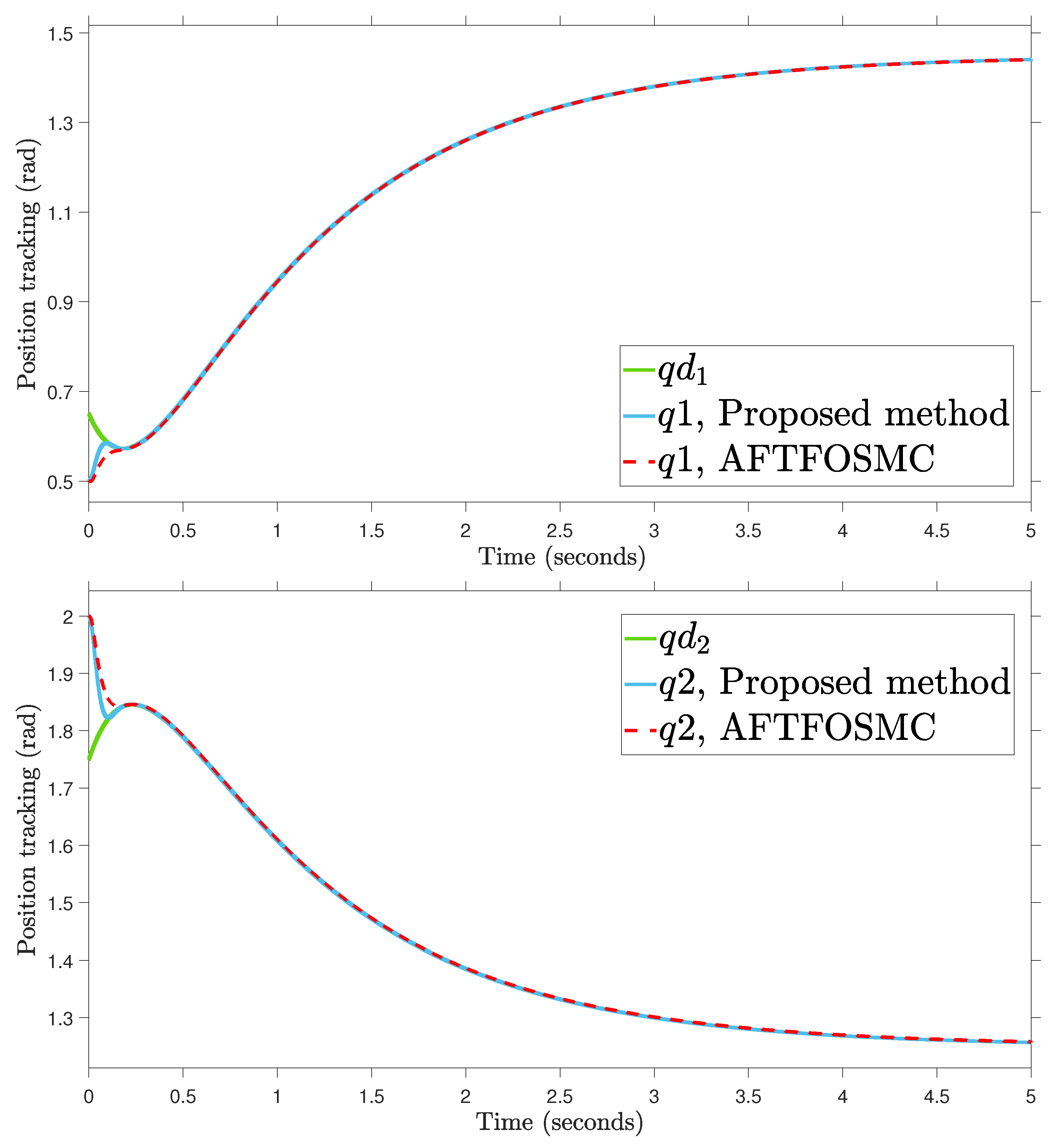
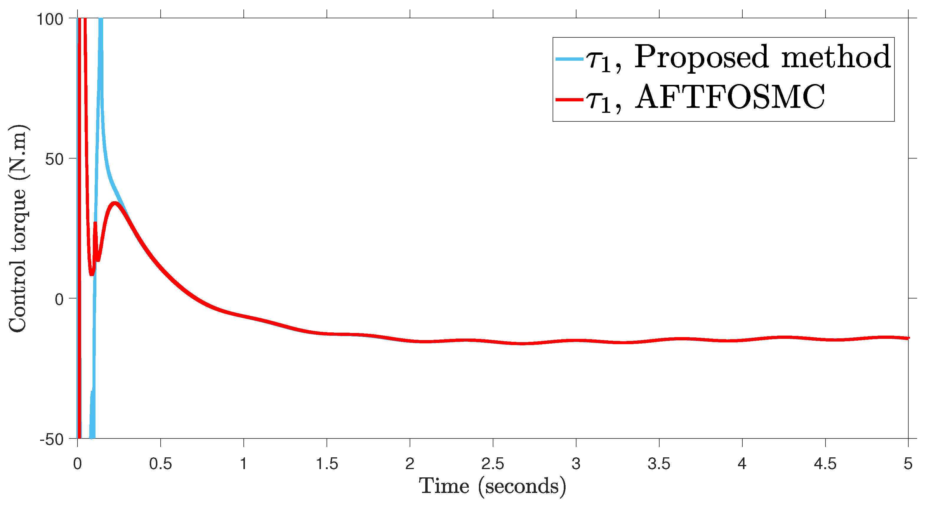
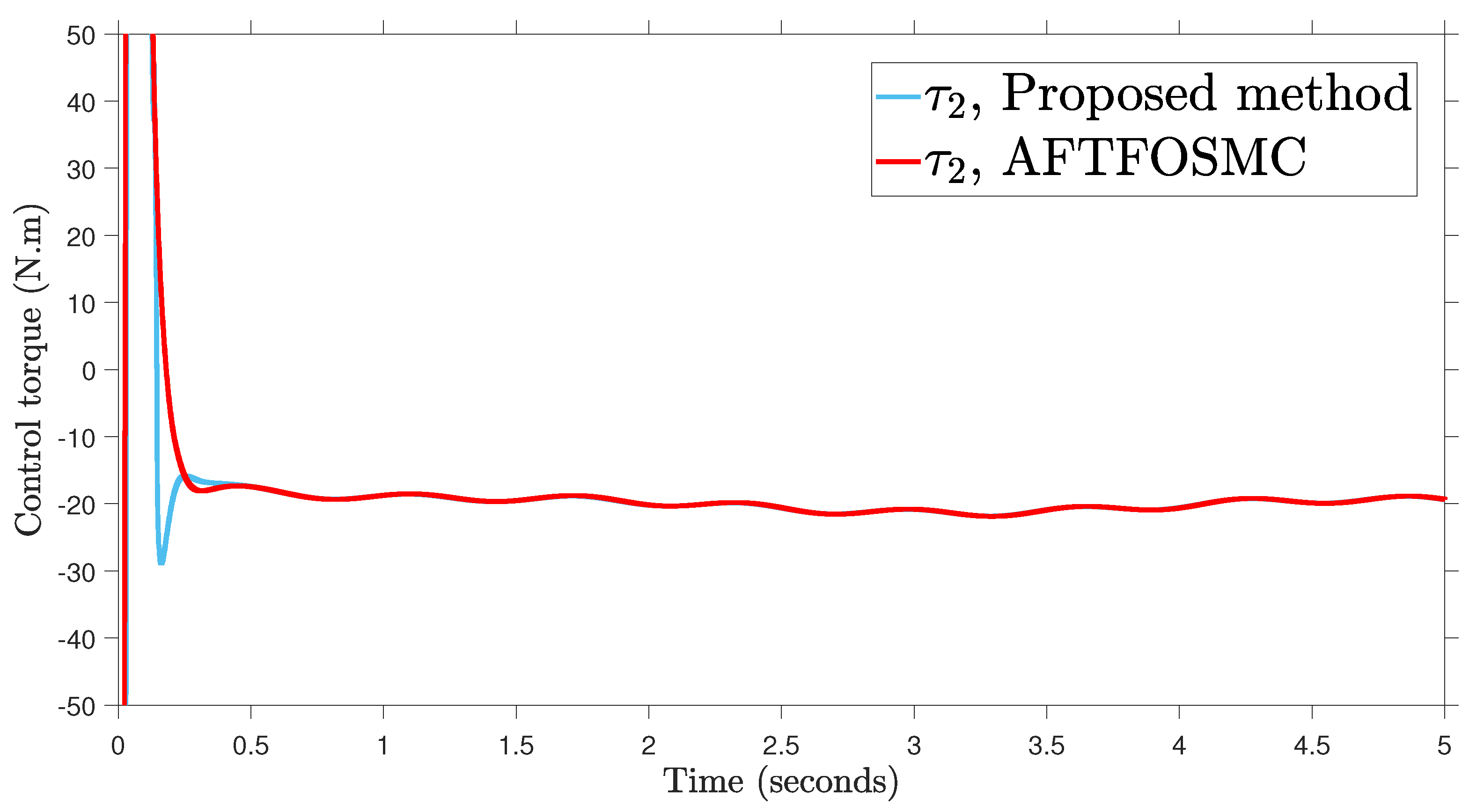
5. Results and Discussions

In order to show the simulation performance and test the suggested AFoIFxTSM technique, a two degree-of-freedom (DOF) manipulator is used to implement the Euler–Lagrange system. A 2-DOF robotic manipulator is utilized in the existence of disturbances and uncertainties depicted in Figure 2. The simulations are given here in order to show how well the AFoIFxTSM works with uncertainties and disturbances. Therefore, MATLAB/Simulink simulations are utilized to explain the outcomes of these analyses. The description of the dynamics of robotic manipulators with 2-DOF is given, together with the control and model parameters (

Table 1. Parameters of AFoIFxTSM.

Parameter	Values
${\sigma }_1$	5
${\sigma }_2$	25
${\sigma }_3$	1
${\alpha }_1$	0.9
${\alpha }_2$	1.1
$\beta$	0.99
${\mu }_1$	10
${\mu }_2$	10
${\mu }_{11}$	0.9
${\mu }_{22}$	1.01
${\sigma }_4$	10
${\sigma }_5$	100
${\gamma }_1$	0.5
${\gamma }_2$	1.1
${\overline{\eta }}_1$	0.1
${\overline{\eta }}_2$	0.1
${\overline{\eta }}_3$	0.1
${\theta }_1\left(0\right)$	0.5
${\theta }_2\left(0\right)$	2

and

Table 2. Parameters of 2-DOF robotic manipulator.

Parameter	Description	Value
$m_{01}$	nominal mass of link 1	0.4 kg
$m_{02}$	nominal mass of link 2	1.2 kg
${\hat{m}}_1$	mass of link 2	0.5 kg
${\hat{m}}_2$	mass of link 2	1.5 kg
$l_1$	length of the link l	1 m
$l_2$	length of the link 2	1 m
$r_1$	centroid length of joint 1	0.5 m
$r_2$	centroid length of joint 2	0.85 m
$J_1$	moment of inertia 1	5 kg·m${}^2$
$J_2$	moment of inertia 2	5 kg·m${}^2$
g	gravitational constant	9.8 m/s${}^2$

), projected trajectories, uncertainties, and disturbances [38]:

$$M\left(\theta \right)=\left[\begin{array}{cc}{M}_{11}& M_{12}\\ M_{21}& M_{22}\end{array}\right],C(\theta ,\dot{\theta })=\left[\begin{array}{c}{C}_1\\ C_2\end{array}\right],G\left(\theta \right)=\left[\begin{array}{c}{G}_1\\ G_2\end{array}\right],$$

$$\tau \left(t\right)=\left[\begin{array}{c}{u}_1\\ u_2\end{array}\right],{\theta }_d=\left[\begin{array}{c}1.45-1.4e^{-t}+0.6e^{-4t}\\ 1.25+e^{-t}-0.5e^{-4t}\end{array}\right],{\tau }_d=\left[\begin{array}{c}0.2sin\left(t\right)+0.5sin\left(10t\right)\\ 0.2cos\left(2t\right)+0.5sin\left(10t\right)\end{array}\right].$$

where $M_{11}=m_1{r}_1^2+m_1(r_1^2+l_1^2)+2cos\left({\theta }_2\right)m_2{l}_1{r}_2^{}+J_1+J_2$, $M_{12}=m_2{r}_2^2+cos\left({\theta }_2\right)m_2{r}_2^{}{l}_1+J_2$, $M_{21}=M_{12}$, $M_{22}=m_2{r}_2^2+J_2$, $C_1=-sin\left({\theta }_2\right)m_2{r}_2^{}{l}_1{\dot{\theta }}_1{\dot{\theta }}_2-sin\left({\theta }_2\right)m_2{r}_2^{}{l}_1({\dot{\theta }}_1+{\dot{\theta }}_2){\dot{\theta }}_2$, $C_2=sin\left({\theta }_2\right)m_2{r}_2^{}{l}_1{\dot{\theta }}_1{\dot{\theta }}_1$, $G_1=cos\left({\theta }_1\right)(m_1{r}_1^{}+m_2{l}_1^{})g+cos({\theta }_1+{\theta }_2)m_2{r}_2^{}g$, $G_2=cos({\theta }_1+{\theta }_2)m_2{r}_2^{}g$.

For the purpose of determining the appropriate value of $\beta$, the angular position performance at the best value of $\beta$ is shown in Figure 3. It demonstrates that the appropriate fractional-order value, which can be chosen with ease, is 0.99 because the intended trajectories do not reach zero tracking errors at fractional-order values of 0.9 and 0.8.

In this paragraph, the proposed AFoIFxTSM method is designed to adjust the uncertain dynamics of the 2-DOF robotic manipulator under unknown external disturbances. This is done in order to ensure that the robot is able to successfully complete its task. The compared simulations are performed with adaptive fractional-order sliding mode control (AFTFOSMC) [34] in order to provide more evidence of the viability of the designed technique. The values for (25) are chosen to be the same as (12), and the parameters of (27) are chosen as ${\overline{\eta }}_1=20$, ${\overline{\eta }}_2=20$, and ${\overline{\eta }}_3=20$. The results are compared between the suggested AFoIFxTSM scheme and the AFTFOSMC method in the presence of unknown dynamics to verify the performance of the desired trajectory tracking, tracking error, control torque inputs, and sliding surfaces presented in Figure 4, Figure 5, Figure 6 and Figure 7, respectively. Moreover, the quantitative results of the tracking errors in terms of the root mean square (RMS) are given in

Table 3. Quantitative tracking error performance.

	AFTFOSMC	Proposed Method
$e_{11RMS}$	0.0093	0.0079
$e_{12RMS}$	0.0153	0.0136
${\sum }_1^2{e}_{1iRMS}$	0.0246	0.0125

. And the depiction of the adaptive gains of the unknown parameters is shown in Figure 8.

According to the findings from Figure 4, Figure 5, Figure 6, Figure 7 and Figure 8 that are compared and demonstrated, the AFoIFxTSM possesses better tracking capability, non-chatter control inputs, and precise adaptive compensation despite the existence of unknown and uncertain dynamics.

Here is an explanation of the simulated results of the suggested AFoIFxTSM scheme. Following the completion of the comparison of the proposed AFoIFxTSM scheme and AFTFOSMC, the constant parameters are adjusted in a manner that is considered appropriate. Looking at Figure 4 and Figure 5 makes it quite clear that the proposed scheme gives less angular position error with the small convergence time that is required. Furthermore, Figure depicts the control performance, and it can easily be observed that the provided method renders the non-chatter and practical control input possible. The adaptive estimation can be seen in Figure 8, which demonstrates that the adaptive rules do not suffer from the issue of drifting.

Now, a concise analysis of the limitations imposed by the proposed controller is presented. These limitations are discussed regarding the proposed controller gain values and stability investigations. The appropriate parameters of the proposed scheme are the ones that are picked within the range that was specified accordingly as ${\sigma }_1>0$, ${\sigma }_2>0$, ${\sigma }_3>0$, $0<{\alpha }_1<1$, ${\alpha }_2>1$, $0<\beta <1$, ${\sigma }_4>0$, ${\sigma }_5>0$, $0<{\gamma }_1<1$ and ${\gamma }_2>1$. If these concerns are disregarded, then the proposed scheme will not be affected, and the system will no longer demonstrate fixed-time stability. It is abundantly obvious, in light of the findings of (23) and (43), that ${\sigma }_i$ is not directly related to $T_1$ and $T_4$ besides the fact that ${\sigma }_i$ is directly to $\tau \left(t\right)$ in (12) and (25). Thus, to simultaneously achieve error convergence in a fixed settling time and overall stability of the system, it is necessary to adjust ${\sigma }_i$ to the appropriate values. Hence, these values are the deciding factor in determining whether or not the system is stable. Since it is known where each of the individual parameters falls within their ranges, it is possible to pick the appropriate value to some extent that is sufficient. This makes the process of choosing the appropriate value feasible.

6. Conclusions

In an attempt to obtain good tracking results for the uncertain Euler–Lagrange system under external disturbance, an AFoIFxTSM is put forward as a potential solution. The proposed scheme converges in a fixed amount of time and obtains the desired tracking performance as a result of using this method. As one of the applications of the Euler–Lagrange system, a 2-DOF robotic manipulator is used, and then AFoIFxTSM is developed for unknown dynamics for the purpose of illustrating the effectiveness of the designed technique. The compared results indicate that the proposed AFoIFxTSM approach is better than the AFTFOSMC method and gives faster response time, lower tracking error, and a greater capacity to ignore sources of uncertainty. Moreover, the study of smooth and non-smooth nonlinearities may be introduced in this area of research on the Euler–Lagrange system, such as highly coupled robotic manipulators, parallel robots, mobile robots, and so on. This would be a significant expansion of the work that was originally proposed.

References

1. Roy, S.; Roy, S.B.; Kar, I.N. Adaptive–robust control of Euler–Lagrange systems with linearly parametrizable uncertainty bound. IEEE Trans. Control Syst. Technol. 2017, 26, 1842–1850. [Google Scholar] [CrossRef]
2. Gao, S.; Song, R.; Li, Y. Coordinated Control of Multiple Euler–Lagrange Systems for Escorting Missions with Obstacle Avoidance. Appl. Sci. 2019, 9, 4144. [Google Scholar] [CrossRef]
3. Li, Y.; Zhao, D.; Zhang, Z.; Liu, J. An IDRA approach for modeling helicopter based on Lagrange dynamics. Appl. Math. Comput. 2015, 265, 733–747. [Google Scholar] [CrossRef]
4. Xuan-Mung, N.; Golestani, M. Smooth, Singularity-Free, Finite-Time Tracking Control for Euler&ndash;Lagrange Systems. Mathematics 2022, 10, 3850. [Google Scholar] [CrossRef]
5. David, S.A.; Valentim, C.A. Fractional Euler-Lagrange Equations Applied to Oscillatory Systems. Mathematics 2015, 3, 258–272. [Google Scholar] [CrossRef]
6. Han, H.; Yin, Z.; Ning, Y.; Liu, H. Development of a 3D Eulerian/Lagrangian Aircraft Icing Simulation Solver Based on OpenFOAM. Entropy 2022, 24, 1365. [Google Scholar] [CrossRef]
7. Shao, X.; Sun, G.; Yao, W.; Liu, J.; Wu, L. Adaptive sliding mode control for quadrotor UAVs with input saturation. IEEE/ASME Trans. Mechatron. 2021, 27, 1498–1509. [Google Scholar] [CrossRef]
8. Choi, T.Y.; Choi, B.S.; Seo, K.H. Position and compliance control of a pneumatic muscle actuated manipulator for enhanced safety. IEEE Trans. Control Syst. Technol. 2010, 19, 832–842. [Google Scholar] [CrossRef]
9. Roy, S.; Kar, I.N.; Lee, J.; Jin, M. Adaptive-robust time-delay control for a class of uncertain Euler–Lagrange systems. IEEE Trans. Ind. Electron. 2017, 64, 7109–7119. [Google Scholar] [CrossRef]
10. Ahmed, S.; Azar, A.T.; Tounsi, M. Adaptive Fault Tolerant Non-Singular Sliding Mode Control for Robotic Manipulators Based on Fixed-Time Control Law. Actuators 2022, 11, 353. [Google Scholar] [CrossRef]
11. Pham, H.V.; Hoang, Q.D.; Pham, M.V.; Do, D.M.; Phi, N.H.; Hoang, D.; Le, H.X.; Kim, T.D.; Nguyen, L. An Efficient Adaptive Fuzzy Hierarchical Sliding Mode Control Strategy for 6 Degrees of Freedom Overhead Crane. Electronics 2022, 11, 713. [Google Scholar] [CrossRef]
12. Gong, B.; Li, S.; Yang, Y.; Shi, J.; Li, W. Maneuver-free approach to range-only initial relative orbit determination for spacecraft proximity operations. Acta Astronaut. 2019, 163, 87–95. [Google Scholar] [CrossRef]
13. Tao, G. Multivariable adaptive control: A survey. Automatica 2014, 50, 2737–2764. [Google Scholar] [CrossRef]
14. Ahmed, S.; Ghous, I.; Mumtaz, F. TDE Based Model-free Control for Rigid Robotic Manipulators under Nonlinear Friction. Sci. Iran. 2022. [Google Scholar] [CrossRef]
15. Gao, H.; Bi, W.; Wu, X.; Li, Z.; Kan, Z.; Kang, Y. Adaptive Fuzzy-Region-Based Control of Euler–Lagrange Systems with Kinematically Singular Configurations. IEEE Trans. Fuzzy Syst. 2020, 29, 2169–2179. [Google Scholar] [CrossRef]
16. Lavretsky, E.; Wise, K.A. Robust adaptive control. In Robust and Adaptive Control: With Aerospace Applications; Springer: London, UK, 2012; pp. 317–353. [Google Scholar]
17. Zhao, D.; Li, S.; Gao, F. A new terminal sliding mode control for robotic manipulators. Int. J. Control 2009, 82, 1804–1813. [Google Scholar] [CrossRef]
18. Feng, Y.; Yu, X.; Man, Z. Non-singular terminal sliding mode control of rigid manipulators. Automatica 2002, 38, 2159–2167. [Google Scholar] [CrossRef]
19. Yu, X.; Zhihong, M. Fast terminal sliding-mode control design for nonlinear dynamical systems. IEEE Trans. Circuits Syst. I Fundam. Theory Appl. 2002, 49, 261–264. [Google Scholar]
20. Yang, L.; Yang, J. Nonsingular fast terminal sliding-mode control for nonlinear dynamical systems. Int. J. Robust Nonlinear Control 2011, 21, 1865–1879. [Google Scholar] [CrossRef]
21. Meghni, B.; Dib, D.; Azar, A.T.; Ghoudelbourk, S.; Saadoun, A. Robust Adaptive Supervisory Fractional Order Controller for Optimal Energy Management in Wind Turbine with Battery Storage. In Fractional Order Control and Synchronization of Chaotic Systems; Studies in Computational Intelligence; Springer International Publishing: Cham, Switzerland, 2017; Volume 688, pp. 165–202. [Google Scholar]
22. Zhang, M.; Zang, H.; Bai, L. A new predefined-time sliding mode control scheme for synchronizing chaotic systems. Chaos Solitons Fractals 2022, 164, 112745. [Google Scholar] [CrossRef]
23. Sami, I.; Ullah, S.; Khan, L.; Al-Durra, A.; Ro, J.S. Integer and fractional-order sliding mode control schemes in wind energy conversion systems: Comprehensive review, comparison, and technical insight. Fractal Fract. 2022, 6, 447. [Google Scholar] [CrossRef]
24. Meghni, B.; Dib, D.; Azar, A.T.; Saadoun, A. Effective supervisory controller to extend optimal energy management in hybrid wind turbine under energy and reliability constraints. Int. J. Dyn. Control 2018, 6, 369–383. [Google Scholar] [CrossRef]
25. Chávez-Vázquez, S.; Gómez-Aguilar, J.F.; Lavín-Delgado, J.; Escobar-Jiménez, R.F.; Olivares-Peregrino, V.H. Applications of fractional operators in robotics: A review. J. Intell. Robot. Syst. 2022, 104, 63. [Google Scholar] [CrossRef]
26. Alzabut, J.; Selvam, A.G.M.; El-Nabulsi, R.A.; Dhakshinamoorthy, V.; Samei, M.E. Asymptotic stability of nonlinear discrete fractional pantograph equations with non-local initial conditions. Symmetry 2021, 13, 473. [Google Scholar] [CrossRef]
27. Ammar, H.H.; Azar, A.T.; Shalaby, R.; Mahmoud, M.I. Metaheuristic Optimization of Fractional Order Incremental Conductance (FO-INC) Maximum Power Point Tracking (MPPT). Complexity 2019, 2019, 1–13. [Google Scholar] [CrossRef]
28. Chen, Y.; Wang, B.; Chen, Y.; Wang, Y. Sliding mode control for a class of nonlinear fractional order systems with a fractional fixed-Time reaching law. Fractal Fract. 2022, 6, 678. [Google Scholar] [CrossRef]
29. Sun, Q.; Liao, T.; Liu, Z.W.; Chi, M.; He, D. Fixed-Time Coverage Control of Mobile Robot Networks Considering the Time Cost Metric. Sensors 2022, 22, 8938. [Google Scholar] [CrossRef] [PubMed]
30. Vo, A.T.; Truong, T.N.; Le, Q.D.; Kang, H.J. Fixed-Time Sliding Mode-Based Active Disturbance Rejection Tracking Control Method for Robot Manipulators. Machines 2023, 11, 140. [Google Scholar] [CrossRef]
31. Sui, B.; Zhang, J.; Li, Y.; Liu, Y.; Zhang, Y. Fixed-Time Trajectory Tracking Control of Unmanned Surface Vessels with Prescribed Performance Constraints. Electronics 2023, 12, 2866. [Google Scholar] [CrossRef]
32. Zhang, D.; Cao, L.; Tang, S. Fractional-order sliding mode control for a class of uncertain nonlinear systems based on LQR. Int. J. Adv. Robot. Syst. 2017, 14, 1729881417694290. [Google Scholar] [CrossRef]
33. Ahmed, S.; Azar, A.T.; Tounsi, M.; Anjum, Z. Trajectory Tracking Control of Euler–Lagrange Systems Using a Fractional Fixed-Time Method. Fractal Fract. 2023, 7, 355. [Google Scholar] [CrossRef]
34. Ahmed, S.; Wang, H.; Tian, Y. Fault tolerant control using fractional-order terminal sliding mode control for robotic manipulators. Stud. Inf. Control 2018, 27, 55–64. [Google Scholar] [CrossRef]
35. Zhang, X.; Huang, W. Adaptive neural network sliding mode control for nonlinear singular fractional order systems with mismatched uncertainties. Fractal Fract. 2020, 4, 50. [Google Scholar] [CrossRef]
36. Abdeljawad, T.; Alzabut, J. On Riemann-Liouville fractional q–difference equations and their application to retarded logistic type model. Math. Methods Appl. Sci. 2018, 41, 8953–8962. [Google Scholar] [CrossRef]
37. Rajchakit, G.; Pratap, A.; Raja, R.; Cao, J.; Alzabut, J.; Huang, C. Hybrid control scheme for projective lag synchronization of Riemann–Liouville sense fractional order memristive BAM NeuralNetworks with mixed delays. Mathematics 2019, 7, 759. [Google Scholar] [CrossRef]
38. Zhai, J.; Li, Z. Fast-exponential sliding mode control of robotic manipulator with super-twisting method. IEEE Trans. Circuits Syst. II Express Briefs 2021, 69, 489–493. [Google Scholar] [CrossRef]
39. Ahmed, S.; Azar, A.T.; Tounsi, M. Design of Adaptive Fractional-Order Fixed-Time Sliding Mode Control for Robotic Manipulators. Entropy 2022, 24, 1838. [Google Scholar] [CrossRef]
40. Su, Y.; Zheng, C.; Mercorelli, P. Robust approximate fixed-time tracking control for uncertain robot manipulators. Mech. Syst. Signal Process. 2020, 135, 106379. [Google Scholar] [CrossRef]
Figure 1. Block diagram of the proposed method.
Fractalfract 07 00712 g001
Figure 2. The 2-DOF robotic manipulator.
Fractalfract 07 00712 g002
Figure 3. Tracking error at different fractional-order parameters.
Fractalfract 07 00712 g003
Figure 4. Position tracking.
Fractalfract 07 00712 g004
Figure 5. Tracking error.
Fractalfract 07 00712 g005
Figure 6. Control input.
Fractalfract 07 00712 g006aFractalfract 07 00712 g006b
Figure 7. Sliding surface.
Fractalfract 07 00712 g007
Figure 8. Adaptive parameter estimation.
Fractalfract 07 00712 g008