A Fractional-Order Telegraph Diffusion Model for Restoring Texture Images with Multiplicative Noise

Abstract

Multiplicative noise removal from texture images poses a significant challenge. Different from the diffusion equation-based filter, we consider the telegraph diffusion equation-based model, which can effectively preserve fine structures and edges for texture images. The fractional-order derivative is imposed due to its textural detail enhancing capability. We also introduce the gray level indicator, which fully considers the gray level information of multiplicative noise images, so that the model can effectively remove high level noise and protect the details of the structure. The well-posedness of the proposed fractional-order telegraph diffusion model is presented by applying the Schauder’s fixed-point theorem. To solve the model, we develop an iterative algorithm based on the discrete Fourier transform in the frequency domain. We give various numerical results on despeckling natural and real SAR images. The experiments demonstrate that the proposed method can remove multiplicative noise and preserve texture well.

1. Introduction

Image multiplicative denoising is an important part of the image preprocessing module and has a wild application in military, medical, and other fields. Multiplicative noise, which is often present in ultrasound, laser, and SAR images, severely destroys the edges and details of the images [1,2,3]. Compared with additive noise, multiplicative noise is more difficult to remove, especially in texture images, because the texture information is often considered as noise in the process of denoising due to its high oscillatory nature. Removing multiplicative noise from texture images poses a challenge for image processing and attracts lots of attention [4,5].

Let $I_0$ be the degraded image on $\mathrm{\Omega }\subset {\mathbb{R}}^2$, I be the corresponding true image, and N denote the noise with mean 1 and variance ${\sigma }^2$. The relationship between the true image and the degraded image can be expressed as

$$I_0=IN.$$

In this paper, we consider multiplicative noise N following gamma distribution, which often exists in SAR images [6]. The probability density function of N is given by

$$p\left(N\right)=\frac{L^L{N}^{L-1}}{\mathsf{\Gamma }\left(L\right)}{e}^{-LN}{\mathbf{1}}_{\{N\ge 0\}},$$

where $L>0$ is a real number denoting the number of “looks”, and ${\mathbf{1}}_{\{N\ge 0\}}$ denotes the indicator function on the subset $\{N\ge 0\}$ [7].

In the past decades, the variational-based methods and the PDE-based methods have been developed as two powerful techniques for image denoising. Currently, there are some popular variational-based methods for the multiplicative noise removal problem. Aubert and Aujol [8] presented a variational denoising model, which was denoted as AA model. This model is based on the total variation (TV) regularization term and the fitting term, where the fitting term was obtained by a maximum a posteriori (MAP) estimation. However, this model is nonconvex except for the condition $I\in (0, 2f)$. To this end, Shi and Osher [9] presented a global strictly convex variational model (SO). They converted the multiplicative noise problem into an additive one by imposing a logarithmic transformation and derived the TV minimization model. Huang et al. [10] also introduced a new total variation (NTV) denoising model by using the modified TV regularization. The objective function they proposed is strictly convex and unconstrained. Dong et al. [11] presented a convex variational (CV) model for image restoration based on the AA model. The authors introduced a quadratic penalty term by considering the statistical properties of the multiplicative Gamma noise.

Some nonlinear diffusion based approaches were also proposed to handle the multiplicative noise removal problems. In [12], they developed a nonlinear coherent diffusion (NCD) model for the noise removal of ultrasound images. By combining the noise level and the image anisotropy, the NCD model changes gradually from isotropic diffusion to anisotropic coherent diffusion and eventually evolves to mean curvature motion. The doubly degenerated (DD) diffusion model, proposed in [13], used both the gradient information and gray level information of the image to remove multiplicative noise. They introduced a new gray level indicator into the diffusion coefficient of the equation. The DD model shows the effectiveness of the PDE based methods in image denoising. Due to the degradation of the edge detector function, the analysis of the well-posedness of such model is usually difficult.

To our knowledge, researchers usually focus on parabolic PDE-based methods for image denoising problems. However, it has been shown that the hyperbolic PDE-based methods are more beneficial to edge detection and can improve the image effect better than parabolic PDEs [14]. In [15], the authors treated the image as an elastic sheet and extended the diffusion equation to the telegraph-diffusion Equation (TDE ). The “telegraph” is derived from the telegraphers’ equation in [16]. The TDE model can be regarded as the interpolating between the diffusion equation and the wave equation. Moreover, it can preserve edges better due to the effect of “force”, which is produced by the second derivative term in time, i.e., the acceleration. However, it is difficult to investigate the existence and uniqueness of the TDE model. To this end, Cao et al. [17] presented an improved parabolic–hyperbolic model by introducing the Gaussian kernel in the edge-controlled function. This model can be seen as a regularized version of the TDE model. The authors proved the well-posedness of their model. Inspired by the TDE model [15] and the fourth-order PDE model in [18], Zeng et al. [19] suggested a class of nonlinear fourth-order telegraph-diffusion equations, which can effectively eliminate the staircase effects and preserve edges. Zhang et al. [20] presented a spatial fractional telegraph equation, which can remove additive noise and preserve the image structures. Moreover, this model avoids “staircase effect” and “speckle effect”. In conclusion, the hyperbolic PDE-based models show priority in additive noise removal. Furthermore, the hyperbolic PDE-based methods were also been used in some multiplicative noise removal problems [5,21], which will be introduced in more detail in Section 3.

In recent years, the fractional-order operator has been widely used and become the focus of research in biomedical, fluid dynamics, material science, and other fields. In material science, Shymanskyi et al. developed a mathematical model of the linear elasticity for capillary-porous materials with fractal structure [22] and Hendy et al. proposed a model of thermo-viscoelasticity with fractional order heat transfer [23]. In biomedical, Zhou et al. constructed a COVID-19 infection model in the framework of fractal fractional derivative [24]. It can be noted that the role of the fractional-order operator has attracted more and more attention in more fields.

Recently, the fractional-order methods have gained lots of recognition in image processing. In general, fractional-order methods dealing with noise removal can be divided into fractional-order methods based on diffusion equation methods and variational methods. In 2008, Bai and Feng (BF) [25] proposed a class of fractional-order anisotropic diffusion models for additive Gaussian noise removal. The models enjoy the intermediate properties of the second and fourth-order anisotropic diffusion equations. Inspired by Cuesta’s method of interpolating between the heat equation and the wave equation using time fractional derivatives [26], Janev generalized the BF model to handle the additive noise removal problem [27]. Their model was able to effectively preserve edges in the highly oscillatory areas. In order to use different derivatives to smooth different image regions, Zhang et al. [28] introduced different orders of fractional derivatives into the regularization term. They proposed a total $\alpha$-order variation regularization model with fractional-order derivative. For other fractional-order variational models in additive noise removal, we refer readers to [29,30,31,32]. The above fractional-order based techniques are usually used to avoid the speckle effect caused by the fourth-order models and the staircase effect caused by the second-order models. Moreover, there is strong evidence to suggest that fractional-order derivatives may be effective tools for texture preservation in image processing [4,33,34,35,36,37]. In particular, fractional-order methods contribute to the multiplicative denoising of texture images [4,37].

It is well known that multiplicative noise is more destructive to image information than additive noise. In addition, textures are usually considered as noise and are erased in the denoising process. Therefore, it is difficult to denoise texture images contaminated by multiplicative noise. To this end, we propose a model combining the telegraph diffusion equation with the fractional-order derivative in this paper. Based on the characteristic of the hyperbolic PDE, the telegraph diffusion equation plays a significant role in texture structure preservation, which is different from the traditional diffusion equation used for image denoising. In the model, the fractional-order derivative is an effective tool for texture detail enhancement. A gray level indicator is introduced into the diffusion coefficient to remove multiplicative noise and preserve structural details. The Gaussian kernel function is also added to the diffusion coefficient, which facilitates the analysis of the well-posedness of our suggested model. An iterative algorithm using the two-dimensional discrete Fourier transform (DFT) in the frequency domain is used to solve the proposed model.

The rest of the paper is organized as follows. In Section 2, we introduce some fundamental notations and definitions. Some related works and the property of telegraph diffusion-based methods are dedicated in Section 3. In Section 4, we propose a fractional-order telegraph diffusion model for tackling the texture images corrupted by multiplicative noise. Moreover, we study the well-posedness of our proposed model. Section 5 gives the numerical implementation in the frequency domain for the model and provides the experimental results and analysis. We conclude this paper in Section 6.

2. Preliminaries

We review the notations used in this paper. We write the Fourier transform $\widehat{f}$ of $f(x,y)$ on two-dimensional periodic domain ${\mathbb{T}}^2={(-\pi ,\pi ]}^2$ as follows

$$\widehat{f}\left(k\right)=\frac{1}{{\left(2\pi \right)}^2}{\int }_{{\mathbb{T}}^2}f(x,y)e^{-ik·(x,y)}\mathrm{d}x\mathrm{d}y.$$

The fractional $\alpha$-order partial derivatives are defined by [25,38]

$$\begin{array}{c}\hfill D_x^{\alpha }f(x,y)=\sum _{k\in {\mathbb{Z}}^2}{\left(i{k}_1\right)}^{\alpha }\widehat{f}\left(k\right)e^{ik·(x,y)},\alpha \in {\mathbb{R}}^{+},\\ \hfill D_y^{\alpha }f(x,y)=\sum _{k\in {\mathbb{Z}}^2}{\left(i{k}_2\right)}^{\alpha }\widehat{f}\left(k\right)e^{ik·(x,y)},\alpha \in {\mathbb{R}}^{+},\end{array}$$

and ${\left(D_x^{\alpha }f(x,y)\right)}^{\ast }$ represents the conjugation of $D_x^{\alpha }f(x,y)$.

For any $\alpha \in {\mathbb{R}}^{+}$, let ${\parallel ·\parallel }_{{\dot{H}}^{\alpha }}$ and ${\parallel ·\parallel }_{H^{\alpha }}$ be defined as [38,39]

$$\begin{array}{c}\hfill {\parallel f\parallel }_{{\dot{H}}^{\alpha }}^2=\sum _{k\in {\mathbb{Z}}^2}{\left|k\right|}^{2\alpha }{|\widehat{f}\left(k\right)|}^2,\\ \hfill {\parallel f\parallel }_{H^{\alpha }}^2={\parallel f\parallel }_{L^2}^2+{\parallel f\parallel }_{{\dot{H}}^{\alpha }}^2,\end{array}$$

and $H^{\alpha }$ represents the Sobolev space of all f for which ${\parallel f\parallel }_{H^{\alpha }}$ is finite. For any Banach space X, $L^p(0,T;X)$ denotes a normed space consisting of all functions $f:[0,T]\to X$ with

$${\parallel f\parallel }_{L^p(0,T;X)}=\left\{\begin{array}{cc}{\left({\int }_0^T{\parallel f\left(t\right)\parallel }_X^p\mathrm{d}t\right)}^{1/p},\hfill & 1\le p<\infty ,\hfill \\ \underset{0\le t\le T}{esssup}{\parallel f\left(t\right)\parallel }_X,\hfill & p=\infty .\hfill \end{array}\right.$$

Denote the dual of $H^{\alpha }$ by ${\left(H^{\alpha }\right)}^{\prime }$ and define the norm

$${\parallel f\parallel }_{{\left(H^{\alpha }\right)}^{\prime }}=\left\{sup\langle f,u\rangle :u\in H^{\alpha },{\parallel u\parallel }_{H^{\alpha }}\le 1\right\}.$$

Throughout this article, we use $L^p\left(1\le p\le \infty \right)$, $H^{\alpha }$, ${\left(H^{\alpha }\right)}^{\prime }$ to denote $L^p\left({\mathbb{T}}^2\right)$, $H^{\alpha }\left({\mathbb{T}}^2\right)$, ${\left(H^{\alpha }\left({\mathbb{T}}^2\right)\right)}^{\prime }$, respectively. We consider the Banach space

$$W(0,T)=\left\{w\in L^{\infty }\left(0,T;H^{\alpha }\right),w_t\in L^{\infty }\left(0,T;L^2\right),w_{tt}\in L^2\left(0,T;{\left(H^{\alpha }\right)}^{\prime }\right)\right\},$$

with the norm

$${\parallel w\parallel }_W={\parallel w\parallel }_{L^{\infty }\left(0,T;H^{\alpha }\right)}+{∥\frac{\partial w}{\partial t}∥}_{L^{\infty }\left(0,T;L^2\right)}+{∥\frac{{\partial }^{2}w}{\partial t^2}∥}_{L^2\left(0,T;{\left(H^{\alpha }\right)}^{\prime }\right)}.$$

3. Some Related Works and Motivation

In this section, we first introduce the application of fractional-order derivatives and telegraph diffusion equations in image processing. Then we present the property of telegraph diffusion-based methods, which motivates us to construct a new framework for handling the multiplicative noise removal problem for texture images.

3.1. Review of Some Related Works

The diffusion equation is essentially used to describe the change in the density of matter in the diffusion phenomenon, which can be derived directly from the conservation law $I_t+\nabla ·\left(J\right)=0$. Here I is the matter density, J is the diffusion flux, and we have $J=-D\nabla I=-\left(D_x{I}_x+D_y{I}_y\right)$ by Fick’s first law in the two-dimensional case. Fick’s first law gives a positive relationship between the diffusion flux and the concentration gradient. However, it is not enough to describe the nonlocal transport processes in physics with the above diffusion flux, they can be adequately described by expressions with the fractional-order diffusion flux. Schumer et al. [40] proposed the fractional Fick’s law:

$$J=-D{\nabla }^{\alpha }I,$$

where $0<\alpha \le 1$, ${\nabla }^{\alpha }=\frac{D_{+}^{\alpha }I+D_{-}^{\alpha }I}{2}$, $D_{+}^{\alpha }$ and $D_{-}^{\alpha }$ are given in the Riemann–Liouville’s sense. To better describe the seepage flow in porous media, the author of [41] proposed a new fractional-order diffusion model in the framework of fractional Fick’s law. The diffusion equation based on the fractional Fick’s law is widely used to describe the nature of anomalous transport processes in heterogeneous porous media [42,43].

Recently, due to the nonlocal property of the fractional-order derivative operator [44], some researchers developed fractional-order-based methods and achieved good performance in texture preservation. In [33], Pu showed that the fractional-order derivative has the textural detail enhancing capability for detecting image edges. Pu et al. [34] also considered a fractional differential method in textural features detection of the digital image. In [35], the rough set based segmentation method delineates the texture regions of the image more accurately. Based on the image segmentation results, the authors proposed an adaptive fractional differential filter capable of effectively enhancing the texture details of the image. Li et al. [36] developed an adaptive fractional-order total variation $l_1$ regularization model for image restoration, which effectively preserves more image details and avoids staircase artifact. A fractional-order nonlinear diffusion Equation (FDE) model with a gray level indicator was proposed by Yao et al. [4], which is used to remove multiplicative noise in texture images. This fractional-order-based model has the effect of better preserving texture details in images. In the framework of combining traditional diffusion with fractional Fick’s law, the authors [37] proposed a fractional-order diffusion equation for handling multiplicative noise removal from texture images. Different from the integer-order derivative, the fractional-order derivative in the denoising model can balance noise sensitivity and detection accuracy by adjusting the orders. It can be concluded that the fractional-order derivative possesses the advantage of protecting texture structures of images.

The telegraph equation based methods can solve the additive noise removal problem, but they cannot be well applied to multiplicative noise removal. To this end, several telegraph equation-based models for removing multiplicative noise are investigated [5,21]. In [21], Majee et al. first suggested an image despeckling model based on the telegraph total variation equation and fuzzy edge detector. They are interested in the following model,

$$\begin{array}{cccc}\hfill & \frac{{\partial }^{2}I}{\partial t^2}+\gamma \frac{\partial I}{\partial t}=div\left(\theta \left(I\right)\frac{\nabla I}{|\nabla I|}\right)-\lambda \left(1-\frac{I_0}{I}\right),\hfill & \hfill & \mathrm{in}{\mathrm{\Omega }}_T:=\mathrm{\Omega }\times (0,T),\hfill \\ \hfill & \frac{\partial I}{\partial \overrightarrow{n}}=0,\hfill & \hfill & \mathrm{on}\partial {\mathrm{\Omega }}_T:=\partial \mathrm{\Omega }\times (0,T),\hfill \\ \hfill & I(x,y,0)=I_0\left(x\right),\frac{\partial I}{\partial t}(x,y,0)=0,\hfill & \hfill & \mathrm{in}\mathrm{\Omega },\hfill \end{array}$$

where $I_0$ is the noise image defined on domain $\mathrm{\Omega }\in {\mathbb{R}}^2$, $\overrightarrow{n}$ is the outer normal vector, $\gamma$ and $\lambda$ are positive parameters, and $\theta$ denotes the fuzzy edge detector function. Unlike the diffusivity function in [21], Majee et al. [5] designed the following equation based on telegraph diffusion (TD),

$$\begin{array}{cccc}\hfill & \frac{{\partial }^{2}I}{\partial t^2}+\gamma \frac{\partial I}{\partial t}=div\left(g\left(I_{\sigma },\left|\nabla I_{\sigma }\right|\right)\nabla I\right),\hfill & \hfill & \mathrm{in}{\mathrm{\Omega }}_T\hfill \\ \hfill & \frac{\partial I}{\partial \overrightarrow{n}}=0,\hfill & \hfill & \mathrm{on}\partial {\mathrm{\Omega }}_T,\hfill \\ \hfill & I(x,y,0)=I_0(x,y),\frac{\partial I}{\partial t}(x,y,0)=0,\hfill & \hfill & \mathrm{in}\mathrm{\Omega }.\hfill \end{array}$$

(1)

Here, $g\left(I_{\sigma },\left|\nabla I_{\sigma }\right|\right)=\frac{2{\left|I_{\sigma }\right|}^{\nu }}{{\left(M_{\sigma }^I\right)}^{\nu }+{\left|I_{\sigma }\right|}^{\nu }}·\frac{1}{1+{\left(\frac{\left|\nabla I_{\sigma }\right|}{K}\right)}^2}$ is the diffusion function, where $I_{\sigma }=G_{\sigma }\ast I$ and $M_{\sigma }^I=\underset{x\in \mathrm{\Omega }}{max}\left|I_{\sigma }(x,t)\right|$. In this case, the gray level indicator function is $b\left(I\right)=\frac{2{\left|I_{\sigma }\right|}^{\nu }}{{\left(M_{\sigma }^I\right)}^{\nu }+{\left|I_{\sigma }\right|}^{\nu }}.$ Equation (1) is a hyperbolic PDE-based model with a gray level indicator, which can overcome the limitations of parabolic PDE based methods and gradient based despeckling methods. This model effectively preserves the edges during the image denoising process.

In addition, Xu et al. [45] discussed two denoising models by combining the parabolic equation and hyperbolic equation for electronic speckle pattern interferometry (ESPI) fringe pattern noise removal. The proposed models are called parabolic–hyperbolic oriented partial differential Equations (PH-OPDEs), which can denoise ESPI fringe images while preserving fringes. In addition, the proposed PH-OPDEs yield good visual effects for the tested image has high fringe density.

3.2. The Property of Telegraph Diffusion Based Methods

To demonstrate the property of telegraph diffusion based methods for preserving texture details in image denoising, we perform a comparative experiment with a one-dimensional signal $I\left(x\right)=sin\left(\frac{\pi x}{2}\right)+1,x\in [0,50]$. For comparison, we use a telegraph diffusion based equation and a non-telegraph diffusion based equation in the experiment. These two models are given separately as follows.

Telegraph diffusion-based model:

$$\begin{array}{cccc}\hfill & \frac{{\partial }^{2}I}{\partial t^2}+b\frac{\partial I}{\partial t}=a\frac{{\partial }^{2}I}{\partial x^2},\hfill & \hfill & \mathrm{in}(0,50)\times (0,T),\hfill \\ \hfill & I(0,t)=I(50,t)=0,\hfill & \hfill & \mathrm{in}(0,T),\hfill \\ \hfill & I(x,0)=I_0\left(x\right),\frac{\partial I(x,0)}{\partial t}=0,\hfill & \hfill & \mathrm{in}(0,50).\hfill \end{array}$$

(2)

Non-telegraph diffusion-based model:

$$\begin{array}{cccc}\hfill & \frac{\partial I}{\partial t}=a\frac{{\partial }^{2}I}{\partial x^2},\hfill & \hfill & \mathrm{in}(0,50)\times (0,T),\hfill \\ \hfill & I(0,t)=I(50,t)=0,\hfill & \hfill & \mathrm{in}(0,T),\hfill \\ \hfill & I(x,0)=I_0\left(x\right),\frac{\partial I(x,0)}{\partial t}=0,\hfill & \hfill & \mathrm{in}(0,50).\hfill \end{array}$$

(3)

In the test, we choose $a=7$, $b=0.01$. As illustrated in Figure 1, the use of the non-telegraph diffusion-based model makes the signal flat and no longer maintains the original oscillations, while the use of the telegraph diffusion-based model preserves most of the oscillations. It is possible to conclude that telegraph diffusion-based models can protect the original oscillation to a greater extent than non-telegraph diffusion-based models. Namely, the model based on the telegraph diffusion equation can avoid over smoothing phenomenon when processing texture images. The telegraph diffusion based approach has the property of protecting high oscillation patterns, which motivates us to build a framework based on the telegraph diffusion equation to remove multiplicative noise for texture images.

4. The FTDE Model and Its Theoretical Analysis

In this section, we propose a new model based on the fractional-order derivative and the telegraph diffusion equation. In addition, we study the existence and uniqueness of the weak solution for the proposed FTDE model.

4.1. The Proposed FTDE Model

In this subsection, we develop a fractional-order telegraph diffusion filter framework, which is used to remove multiplicative noise for texture images. We use the following gray level indicator and the source term:

$$c\left(I\right)=\frac{{\left|I\right|}^r}{{\left(M^I\right)}^r},$$

and

$$h(I_0,I)=\frac{I_0-I}{I^2},$$

where $M^I=\underset{x,y\in \mathrm{\Omega }}{max}\left|I(x,y,t)\right|$, the parameter r is a positive constant, and $I_0$ is the noise image. We first give the following model:

$$\begin{array}{cccc}\hfill & \frac{{\partial }^{2}I}{\partial t^2}+b\frac{\partial I}{\partial t}={div}^{\alpha }\left(\frac{{\left|I\right|}^r}{{\left(M^I\right)}^r}\frac{1}{1+k{\left|{\nabla }^{\alpha }I\right|}^{\beta }}{\nabla }^{\alpha }I\right)+\lambda \frac{I_0-I}{I^2},\hfill & \hfill & \mathrm{in}{\mathbb{T}}^2\times (0,T),\hfill \\ \hfill & I(x+2\pi ,y,t)=I(x,y,t)=I(x,y+2\pi ,t),\hfill & \hfill & \mathrm{in}{\mathbb{T}}^2\times (0,T),\hfill \\ \hfill & I(x,y,0)=I_0(x,y),\frac{\partial I(x,y,0)}{\partial t}=0,\hfill & \hfill & \mathrm{in}{\mathbb{T}}^2,\hfill \end{array}$$

(4)

where $0<\alpha <2, 0<\beta <1, b>0, k>0, \lambda >0$, ${\nabla }^{\alpha }I=\left(D_x^{\alpha }I,D_y^{\alpha }I\right)$ is the fractional-order derivative operator with $\left|{\nabla }^{\alpha }I\right|=\sqrt{{\left|D_x^{\alpha }I\right|}^2+{\left|D_y^{\alpha }I\right|}^2}$, ${div}^{\alpha }(\overrightarrow{v}(x,y))=-D_x^{\alpha \ast }\left(v_1(x,y)\right)-D_y^{\alpha \ast }\left(v_2(x,y)\right)$, $\overrightarrow{v}(x,y)=\left(v_1(x,y),v_2(x,y)\right)$, and $D_x^{\alpha \ast }$, $D_y^{\alpha \ast }$ is the adjoint of $D_x^{\alpha }$, $D_y^{\alpha }$, respectively.

To be noticed, the fractional-order diffusion equation can better balance detection accuracy and noise sensitivity than the classical integer-order diffusion methods because of the flexibility to adjust the order. When we choose a fixed order $\alpha$$(1<\alpha <2)$, the fractional-order diffusion equation interpolates between the second-order equation and the fourth-order equation. In other words, the fractional-order diffusion equation can effectively avoid speckle effects and staircase effects. Because the fractional derivative at a point is determined by the characteristics of the entire function, not just by the values near that point, the fractional derivative operator has the nonlocal property [44]. Therefore, the model based on the fractional-order diffusion equation can obtain better results in enhancing texture details.

In fact, the telegraph diffusion equation is a parabolic-hyperbolic PDE, which can be viewed as interpolating between the diffusion equation and the wave equation. The telegraph diffusion equation combines diffusion behavior with wave propagation behavior. Compared with other diffusion-based methods, the telegraph diffusion equation preserves the edges and some details better [5]. In particular, the wave nature of the telegraph diffusion equation is beneficial to preserve high oscillatory and textures.

Different from the additive noise image, the variance of the multiplicative noise image is affected by the gray levels of the original image [13]. Therefore, we introduce the gray level indicator $c\left(I\right)$ in our model. In low gray level regions, the value of the gray level indicator becomes very small, which makes the diffusion coefficient very small. Differently, $c\left(I\right)$ will approach 1 in high gray level areas, which causes $\frac{1}{1+k{\left|{\nabla }^{\alpha }I\right|}^{\beta }}$ to dominate the diffusion coefficient. As we know, the value $\frac{1}{1+k{\left|{\nabla }^{\alpha }I\right|}^{\beta }}$ will change depending on the gradient information. We use the fidelity term $H(I_0,I)={\int }_{{\mathbb{T}}^2}\left(logI+\frac{I_0}{I}\right)$ in [8]. Accordingly, the source term in the diffusion equation is $h(I_0,I)=\frac{I_0-I}{I^2},$ which can steer the multiplicative denoising process.

The edge indicator ${\nabla }^{\alpha }I$ is very sensitive to noise, which causes it to treat isolated extreme low points of the higher areas as edges to be enhanced or preserved [46]. In addition, the discussed model (4) may be an ill-posed problem due to the degeneracy of the diffusion coefficient [47]. To solve these problems, we introduce the Gaussian kernel function in the diffusion coefficient of the model (4).

In this paper, we propose the following fractional-order telegraph diffusion Equation (FTDE) for multiplicative noise removal:

$$\begin{array}{ccc}\hfill \frac{{\partial }^{2}I}{\partial t^2}+b\frac{\partial I}{\partial t}={div}^{\alpha }\left(\frac{|I_{\sigma }{|}^r}{{\left(M_{\sigma }^I\right)}^r}\frac{1}{1+k{\left|{\nabla }^{\alpha }{I}_{\sigma }\right|}^{\beta }}{\nabla }^{\alpha }I\right)+\lambda \frac{I_0-I}{I^2},& & \mathrm{in}{\mathbb{T}}^2\times (0,T),\hfill \end{array}$$

(5)

$$\begin{array}{ccc}\hfill I(x+2\pi ,y,t)=I(x,y,t)=I(x,y+2\pi ,t),& & \mathrm{in}{\mathbb{T}}^2\times (0,T),\hfill \end{array}$$

(6)

$$\begin{array}{ccc}\hfill I(x,y,0)=I_0(x,y),\frac{\partial I(x,y,0)}{\partial t}=0,& & \mathrm{in}{\mathbb{T}}^2,\hfill \end{array}$$

(7)

where $I_{\sigma }=G_{\sigma }\ast I,M_{\sigma }^I=\underset{x,y\in {\mathbb{T}}^2}{max}\left|I_{\sigma }(x,y,t)\right|$.

The proposed model with the Gaussian kernel can compromise the effect of multiplicative noise and lead to a well-posed problem. Moreover, the model (5)–(7) shares some similar advantages with the model (4). Because of the wave property of the telegraph diffusion equation and the non-local property of fractional derivative, the model (5)–(7) can preserve the oscillation and texture patterns more effectively. In the model, the gray level indicator leads to different diffusion behaviors in different gray level areas, which helps to preserve some details in low gray level areas.

4.2. Existence and Uniqueness of the Solution

In spite of the encouraging results obtained by the FDE method [4], it is difficult to establish the well-posedness of the model. Next, we prove the existence and uniqueness of the weak solution of the FTDE model (5)–(7) by utilizing Schauder–Tikhonov’s fixed-point theorem [48]. Without loss of generality, we assume $b=\lambda =1$ in (5).

Definition 1. 

A function I is called a weak solution of (5)–(7) if there exists $I\in W(0,T)$ such that

$$\begin{array}{ccc}& & 〈\frac{{\partial }^{2}I}{\partial t^2},\varphi 〉+{\int }_{{\mathbb{T}}^2}\left(\frac{\partial I}{\partial t}\varphi +\frac{|I_{\sigma }{|}^r}{{\left(M_{\sigma }^I\right)}^r}\frac{1}{1+k{\left|{\nabla }^{\alpha }{I}_{\sigma }\right|}^{\beta }}{\nabla }^{\alpha }I·{\nabla }^{\alpha }\varphi \right)\mathrm{d}x\mathrm{d}y={\int }_{{\mathbb{T}}^2}\left(\frac{I_0-I}{I^2}\right)\varphi \mathrm{d}x\mathrm{d}y,\hfill \\ & & I(x,y,0)=I_0(x,y),\frac{\partial I(x,y,0)}{\partial t}=0,\mathrm{in}{\mathbb{T}}^2,\hfill \end{array}$$

for a.e. $t\in (0, T)$ and all $\varphi \in H^{\alpha }$.

In the following, we assume that the initial value $I_0\in H^{\alpha }$ satisfies:

$$0<l:=\underset{x,y\in {\mathbb{T}}^2}{inf}{I}_0(x,y) \mathrm{and} d:=\underset{x,y\in {\mathbb{T}}^2}{sup}{I}_0(x,y)<\infty .$$

(8)

Next, let ${\parallel w\parallel }_a:={\parallel w\parallel }_{L^{\infty }\left(0,T;H^{\alpha }\right)}+{∥\frac{\partial w}{\partial t}∥}_{L^{\infty }\left(0,T;L^2\right)}$ and $\overline{N}$ be a positive constant. Then, we define

$$W_{\overline{N}}=\left\{w\in {W(0,T):\parallel w\parallel }_a\le \overline{N}{∥I_0∥}_{H^{\alpha }},l\le w(x,y,t)\le d,\mathrm{a}.\mathrm{e}.\mathrm{in}{\mathbb{T}}^2\times (0,T)\right\}.$$

Let $w\in W_{\overline{N}}$. We consider the linearized problem $P_w$ as follows:

$$\begin{array}{c}\hfill \frac{{\partial }^{2}I}{\partial t^2}+\frac{\partial I}{\partial t}-{div}^{\alpha }\left(h_w{\nabla }^{\alpha }I\right)=\frac{I_0-I}{w^2},\mathrm{in}{\mathbb{T}}^2\times (0,T),\end{array}$$

(9)

with the condition (7), where $h_w(x,y,t):=\frac{{\left|w_{\sigma }\right|}^r}{{\left(M_{\sigma }^w\right)}^r}\frac{1}{1+k{\left|{\nabla }^{\alpha }{w}_{\sigma }\right|}^{\beta }}$.

Lemma 1. 

Assume that I is a weak solution of the problem $P_w$, then

$$0<l\le I(x,y,t)\le d\mathrm{for}\mathrm{a}.\mathrm{e}.(x,y,t)\in {\mathbb{T}}^2\times (0,T).$$

Proof. 

We define ${\left(G\right)}_{+}=max\{0,G\}$. Integrating Equation (9) with respect to the time variable, using (7), multiplying it by ${(I-d)}_{+}$ and integrating over ${\mathbb{T}}^2$, we obtain that

$$\begin{array}{cc}\hfill & \frac{1}{2}\frac{\mathrm{d}}{\mathrm{d}t}{\int }_{{\mathbb{T}}^2}{\left|{\left(I-d\right)}_{+}\right|}^2\mathrm{d}x\mathrm{d}y+{\int }_{{\mathbb{T}}^2}\left(I-I_0\right){\left(I-d\right)}_{+}\mathrm{d}x\mathrm{d}y\hfill \\ \hfill +& {\int }_0^t{\int }_{\left\{I\ge d\right\}}{h}_w{\left|{\nabla }^{\alpha }I\right|}^2\mathrm{d}x\mathrm{d}y\mathrm{d}s+{\int }_0^t{\int }_{\left\{I\ge d\right\}}\left(\frac{I-I_0}{w^2}\right){\left(I-d\right)}_{+}\mathrm{d}x\mathrm{d}y\mathrm{d}s=0.\hfill \end{array}$$

(10)

Noting that $h_w\ge 0$ and $\left(I-I_0\right){\left(I-d\right)}_{+}\ge 0$, we obtain $\frac{\mathrm{d}}{\mathrm{d}t}{\int }_{{\mathbb{T}}^2}{\left|{\left(I-d\right)}_{+}\right|}^2\mathrm{d}x\mathrm{d}y\le 0$. Due to $I_0\le d$, we have ${\int }_{{\mathbb{T}}^2}{\left|{\left(I-d\right)}_{+}\right|}^2\mathrm{d}x\mathrm{d}y\le 0$. Thus, $I(x,y,t)\le d$ for a.e. $(x,y,t)\in {\mathbb{T}}^2\times (0,T)$.

Similarly, defining ${\left(G\right)}_{-}=min\{0,G\}$, integrating Equation (9) with respect to the time variable, multiplying it by ${(I-l)}_{-}$, and integrating over ${\mathbb{T}}^2$, we obtain $0<l\le I(x,y,t)$ for a.e. $(x,y,t)\in {\mathbb{T}}^2\times (0,T)$.    □

Lemma 2. 

The following inequalities hold:

(i) 

$0<a\le h_w\le 1$,

(ii) 

$\left|\frac{\partial h_w}{\partial t}\right|\le C_0$,

where the positive constant$C_0$only depends on$G_{\sigma },I_0,\overline{N},k,l,d,r$and β.

Proof. 

(i) Let $w\in W_{\overline{N}}$. Since $0<l\le w$, $G_{\sigma }$ is positive and the convolution property, we obtain

$$l{∥G_{\sigma }∥}_{L^1}=\left|G_{\sigma }\ast l\right|\le \left|w_{\sigma }\right|\le C_{\sigma }\overline{N}{∥I_0∥}_{H^{\alpha }},$$

$$\left|{\nabla }^{\alpha }{w}_{\sigma }\right|\le \left|\left({\nabla }^{\alpha }{G}_{\sigma }\right)\ast w\right|\le C_{\sigma }\overline{N}{∥I_0∥}_{H^{\alpha }}.$$

By the definition $M_{\sigma }^w={\displaystyle \underset{x,y\in {\mathbb{T}}^2}{max}}\left|w_{\sigma }(x,y,t)\right|$, we have

$$\frac{l^r{∥G_{\sigma }∥}_{L^1}^r}{{\overline{N}}^r{C}_{\sigma }^r{∥I_0∥}_{H^{\alpha }}^r}\le \frac{{\left|w_{\sigma }\right|}^r}{{\left(M_{\sigma }^w\right)}^r}\le 1,$$

and

$$\frac{1}{1+k{\overline{N}}^{\beta }{C}_{\sigma }^{\beta }{∥I_0∥}_{H^{\alpha }}^{\beta }}\le \frac{1}{1+k{\left|{\nabla }^{\alpha }{w}_{\sigma }\right|}^{\beta }}\le 1.$$

Now, we set $a=\frac{l^r{∥G_{\sigma }∥}_{L^1}^r}{{\overline{N}}^r{C}_{\sigma }^r{∥I_0∥}_{H^{\alpha }}^r}·\frac{1}{1+k{\overline{N}}^{\beta }{C}_{\sigma }^{\beta }{∥I_0∥}_{H^{\alpha }}^{\beta }}$, therefore, $0<a\le h_w\le 1$.

(ii) Notice that

$$\left|\frac{\partial h_w}{\partial t}\right|\le r\frac{{\left|w_{\sigma }\right|}^{r-1}\left|G_{\sigma }\ast \frac{\partial w}{\partial t}\right|}{{\left(M_{\sigma }^w\right)}^{2r}}+C\left(\sigma ,\overline{N},k\right){∥I_0∥}_{H^{\alpha }}^{\beta }\equiv A+C\left(\sigma ,\overline{N},k\right){∥I_0∥}_{H^{\alpha }}^{\beta }.$$

According to $w\in W_{\overline{N}}$ and the property of convolution, we see that

$$A\le \left\{\begin{array}{cccc}\hfill & \frac{r{\left(C_{\sigma }\overline{N}{∥I_0∥}_{H^{\alpha }}\right)}^r}{l^{2r}},\hfill & \hfill & \mathrm{if}r>1,\hfill \\ \hfill & \frac{r{C}_{\sigma }\overline{N}{∥I_0∥}_{H^{\alpha }}}{l^{1-r}{∥G_{\sigma }∥}_{L^1}^{1-r}·l^{2r}},\hfill & \hfill & \mathrm{if}0<r\le 1.\hfill \end{array}\right.$$

(11)

Hence, $\left|\frac{\partial h_w}{\partial t}\right|\le C_0$.    □

We can prove the linearized problem (9) has a unique weak solution $I\in W(0,T)$ by applying the Galerkin’s method [49,50,51,52].

Lemma 3. 

The linearized problem (9) admits a unique weak solution $I\in W(0,T)$ such that

(i) ${\parallel I\parallel }_{L^{\infty }\left(0,T;H^{\alpha }\right)}+{∥\frac{\partial I}{\partial t}∥}_{L^{\infty }\left(0,T;L^2\right)}\le C{∥I_0∥}_{H^{\alpha }},$

(ii) ${\int }_0^T{∥\frac{{\partial }^{2}I}{\partial t^2}∥}_{{\left(H^{\alpha }\right)}^{\prime }}^2\mathrm{d}t\le CT{∥I_0∥}_{H^{\alpha }}^2+\overline{C},$

where constant $\overline{C}>0$ and positive constant C only depends on $I_0$, $G_{\sigma }$, l, $\overline{N}$, k, r, β.

Proof. 

(i) Multiplying (9) by $\frac{\partial I}{\partial t}$ and integrating by parts, we obtain

$$\begin{array}{cc}\hfill & \frac{1}{2}\frac{\mathrm{d}}{\mathrm{d}t}{∥\frac{\partial I}{\partial t}∥}_{L^2}^2+{∥\frac{\partial I}{\partial t}∥}_{L^2}^2+{\int }_{{\mathbb{T}}^2}{h}_w{\nabla }^{\alpha }I·{\nabla }^{\alpha }\left(\frac{\partial I}{\partial t}\right)\mathrm{d}x\mathrm{d}y\hfill \\ \hfill =& {\int }_{{\mathbb{T}}^2}\left(\frac{I_0-I}{w^2}\right)\frac{\partial I}{\partial t}\mathrm{d}x\mathrm{d}y\le \frac{1}{2}{∥\frac{I_0-I}{w^2}∥}_{L^2}^2+\frac{1}{2}{∥\frac{\partial I}{\partial t}∥}_{L^2}^2.\hfill \end{array}$$

(12)

Due to integration by parts formula and Lemma 2 (ii), we have

$$\begin{array}{cc}\hfill {\int }_{{\mathbb{T}}^2}{h}_w{\nabla }^{\alpha }I·{\nabla }^{\alpha }\left(\frac{\partial I}{\partial t}\right)\mathrm{d}x\mathrm{d}y& =\frac{1}{2}\frac{\mathrm{d}}{\mathrm{d}t}{\int }_{{\mathbb{T}}^2}{h}_w{\left|{\nabla }^{\alpha }I\right|}^2\mathrm{d}x\mathrm{d}y-\frac{1}{2}{\int }_{{\mathbb{T}}^2}\frac{\partial h_w}{\partial t}{\left|{\nabla }^{\alpha }I\right|}^2\mathrm{d}x\mathrm{d}y\hfill \\ \hfill & \ge \frac{1}{2}\frac{\mathrm{d}}{\mathrm{d}t}{\int }_{{\mathbb{T}}^2}{h}_w{\left|{\nabla }^{\alpha }I\right|}^2\mathrm{d}x\mathrm{d}y-\frac{C_0}{2}{∥{\nabla }^{\alpha }I\left(t\right)∥}_{L^2}^2.\hfill \end{array}$$

(13)

Since $w\in W_{\overline{N}}$ and Lemma 1, we obtain

$$\begin{array}{cc}\hfill {∥\frac{I_0-I}{w^2}∥}_{L^2}^2& \le \frac{1}{l^4}{∥I_0-I∥}_{L^2}^2\hfill \\ \hfill & \le \frac{2}{l^4}\left({∥I_0∥}_{H^{\alpha }}^2+{\parallel I\parallel }_{L^2}^2\right)\hfill \\ \hfill & \le \frac{2}{l^4}{∥I_0∥}_{H^{\alpha }}^2+C{d}^2.\hfill \end{array}$$

(14)

According to the estimates (12)–(14), we observe that

$$\begin{array}{cc}\hfill & \frac{\mathrm{d}}{\mathrm{d}t}\left[{∥\frac{\partial I}{\partial t}∥}_{L^2}^2+{\int }_{{\mathbb{T}}^2}{h}_w{\left|{\nabla }^{\alpha }I\right|}^2\mathrm{d}x\mathrm{d}y\right]\hfill \\ \hfill \le & {∥\frac{I_0-I}{w^2}∥}_{L^2}^2+{∥\frac{\partial I}{\partial t}∥}_{L^2}^2+C_0{∥{\nabla }^{\alpha }I\left(t\right)∥}_{L^2}^2\hfill \\ \hfill \le & \frac{2}{l^4}{∥I_0∥}_{H^{\alpha }}^2+C{d}^2+C_0{∥{\nabla }^{\alpha }I\left(t\right)∥}_{L^2}^2+{∥\frac{\partial I}{\partial t}∥}_{L^2}^2\hfill \\ \hfill =& C+C_0{∥{\nabla }^{\alpha }I\left(t\right)∥}_{L^2}^2+{∥\frac{\partial I}{\partial t}∥}_{L^2}^2.\hfill \end{array}$$

(15)

Noting that $0<a\le h_w$ in Lemma 2, we see

$${∥{\nabla }^{\alpha }I\left(t\right)∥}_{L^2}^2\le \frac{1}{a}{\int }_{{\mathbb{T}}^2}{h}_w{\left|{\nabla }^{\alpha }I\right|}^2\mathrm{d}x\mathrm{d}y.$$

(16)

Combining (15) and (16), we have

$$\frac{\mathrm{d}}{\mathrm{d}t}\left[{∥\frac{\partial I}{\partial t}∥}_{L^2}^2+{\int }_{{\mathbb{T}}^2}{h}_w{\left|{\nabla }^{\alpha }I\right|}^2\mathrm{d}x\mathrm{d}y\right]\le C+C_1\left({∥\frac{\partial I}{\partial t}∥}_{L^2}^2+{\int }_{{\mathbb{T}}^2}{h}_w{\left|{\nabla }^{\alpha }I\right|}^2\mathrm{d}x\mathrm{d}y\right),$$

where $C_1=max\left\{1,\frac{C_0}{a}\right\}$. According to Gronwall’s Lemma, we have

$${∥\frac{\partial I\left(t\right)}{\partial t}∥}_{L^2}^2+{\int }_{{\mathbb{T}}^2}{h}_w(x,y,t){\left|{\nabla }^{\alpha }I(x,y,t)\right|}^2\mathrm{d}x\mathrm{d}y\le e^{C_{1}t}\left(C_2+tC\right),$$

for a.e. $t\in (0,T]$, where $C_2={∥\frac{\partial I\left(0\right)}{\partial t}∥}_{L^2}^2+{\int }_{{\mathbb{T}}^2}{h}_w(x,y,0){\left|{\nabla }^{\alpha }I(x,y,0)\right|}^2\mathrm{d}x\mathrm{d}y.$ With the Inequality (16), we obtain

$${∥{\nabla }^{\alpha }I\left(t\right)∥}_{L^2}^2\le \frac{1}{a}{e}^{C_{1}t}\left(C_2+tC\right).$$

Therefore, for a.e. $t\in (0,T]$,

$${∥\frac{\partial I\left(t\right)}{\partial t}∥}_{L^2}^2+{∥{\nabla }^{\alpha }I\left(t\right)∥}_{L^2}^2\le K_0{e}^{C_{1}t}\left(C_2+tC\right),$$

(17)

where $K_0=max\left\{\frac{1}{a},1\right\}$. Combining $I(x,y,t)=I(x,y,0)+{\int }_0^t\frac{\partial I}{\partial s}\mathrm{d}s$, Young’s inequality and (17), we have

$$\begin{array}{cc}\hfill {∥I\left(t\right)∥}_{L^2}^2& \le 2{∥I_0∥}_{H^{\alpha }}^2+2T{\int }_0^t{∥\frac{\partial I\left(s\right)}{\partial s}∥}_{L^2}^2\mathrm{d}s\hfill \\ \hfill & \le 2{∥I_0∥}_{H^{\alpha }}^2+2T^2{K}_0{e}^{C_{1}T}\left(C_2+TC\right).\hfill \end{array}$$

(18)

From (17) and (18), we conclude that

$${\parallel I\parallel }_{L^{\infty }\left(0,T;H^{\alpha }\right)}+{∥\frac{\partial I}{\partial t}∥}_{L^{\infty }\left(0,T;L^2\right)}\le C{∥I_0∥}_{H^{\alpha }}.$$

(19)

(ii) Multiplying (9) by $\varphi \in H^{\alpha }$ with ${\parallel \varphi \parallel }_{H^{\alpha }}\le 1$, applying Cauchy–Schwarz’s inequality and combining (14) and (19), we find

$$\begin{array}{cc}\hfill \left|〈\frac{{\partial }^{2}I}{\partial t^2},\varphi 〉\right|& \le \left({∥\frac{\partial I}{\partial t}∥}_{L^2}+\left|h_w\right|{∥{\nabla }^{\alpha }I\left(t\right)∥}_{L^2}+{∥\frac{I_0-I}{w^2}∥}_{L^2}\right){\parallel \varphi \parallel }_{H^{\alpha }}\hfill \\ & \le \left\{\left(2C+\sqrt{\frac{2}{l^4}}\right){∥I_0∥}_{H^{\alpha }}+\sqrt{C}d\right\}{\parallel \varphi \parallel }_{H^{\alpha }}.\hfill \end{array}$$

Therefore, we have

$${∥\frac{{\partial }^{2}I}{\partial t^2}∥}_{{\left(H^{\alpha }\right)}^{\prime }}\le C{∥I_0∥}_{H^{\alpha }}+\overline{C}.$$

(20)

Furthermore, by squaring and integrating over $(0,T)$ for (20), it follows that

$${\int }_0^T{∥\frac{{\partial }^{2}I}{\partial t^2}∥}_{{\left(H^{\alpha }\right)}^{\prime }}^2\mathrm{d}t\le CT{∥I_0∥}_{H^{\alpha }}^2+\overline{C}.$$

   □

Theorem 1. 

Assuming that $I_0\in H^{\alpha }$ and (8) hold, the problem (5)–(7) has a weak solution $I\in W(0,T)$.

Proof. 

We first define the space U

$$\begin{array}{c}\hfill U=\left\{w\in L^2\left(0,T;H^{\alpha }\right),\frac{\partial w}{\partial t}\in L^2\left(0,T;L^2\right),\frac{{\partial }^{2}w}{\partial t^2}\in L^2\left(0,T;{\left(H^{\alpha }\right)}^{\prime }\right)\right\}.\end{array}$$

It follows that $U\subset \subset L^2({\mathbb{T}}^2\times (0,T))$. Next, we give the subset $W_M$ of U,

$$\begin{array}{c}\hfill W_M=\left\{{\parallel w\parallel }_{L^2\left(0,T;H^{\alpha }\right)}+{∥\frac{\partial w}{\partial t}∥}_{L^2\left(0,T;L^2\right)}\le C{∥I_0∥}_{H^{\alpha }};{∥\frac{{\partial }^{2}w}{\partial t^2}∥}_{L^2\left(0,T;{\left(H^{\alpha }\right)}^{\prime }\right)}\le C;\right.\\ \hfill \left.0<l\le w(x,y,t)\le d\mathrm{for}\mathrm{a}.\mathrm{e}.(x,y,t)\in {\mathbb{T}}^2\times (0,T),w\left(0\right)=I_0,\frac{\partial w\left(0\right)}{\partial t}=0\right\}.\end{array}$$

Furthermore, we can know that $W_M$ is a nonempty, closed convex, and weakly compact subset of U. Next, we construct the following mapping

$$\begin{array}{cc}\hfill F:& W_M\to W_M\hfill \\ & w\mapsto I_w.\hfill \end{array}$$

In order to use Schauder–Tikhonov’s fixed-point theorem, we need to prove that the mapping $F:w\to I_w$ is weakly continuous from $W_M$ into $W_M$, i.e., if $w_j\rightharpoonup w$ weakly in $W_M$ then $F\left(w_j\right)\rightharpoonup F\left(w\right)$ weakly in $W_M$. Denote $F\left(w_j\right)=I_j$. Thanks to Lemma 3, we can use classical results of compact inclusion in Sobolev spaces [49] to extract the subsequences of $\left\{w_j\right\}$ and $\left\{I_j\right\}$ (still denoted by $\left\{w_j\right\}$ and $\left\{I_j\right\}$), we have

$$\begin{array}{cc}& w_j\rightharpoonup w\mathrm{weakly}\mathrm{in}{L}^2\left((0,T);H^{\alpha }\right),\hfill \\ & \frac{\partial w_j}{\partial t}\rightharpoonup \frac{\partial w}{\partial t}\mathrm{weakly}\mathrm{in}{L}^2\left((0,T);{\left(H^{\alpha }\right)}^{\prime }\right),\hfill \\ & w_j\to w\mathrm{in}{L}^2\left((0,T);L^2\right),\hfill \\ & G_{\sigma }\ast w_j⟶G_{\sigma }\ast w\mathrm{in}{L}^2\left(0,T;L^2\right),\hfill \\ & I_j\rightharpoonup I\mathrm{weakly}\mathrm{in}{L}^2\left((0,T);H^{\alpha }\right),\hfill \\ & \frac{\partial I_j}{\partial t}\rightharpoonup \frac{\partial I}{\partial t}\mathrm{weakly}\mathrm{in}{L}^2\left((0,T);L^2\right),\hfill \\ & \frac{{\partial }^2{I}_j}{\partial t^2}\rightharpoonup \frac{{\partial }^{2}I}{\partial t^2}\mathrm{weakly}\mathrm{in}{L}^2\left((0,T);{\left(H^{\alpha }\right)}^{\prime }\right),\hfill \\ & I_j\to I\mathrm{in}{L}^2\left((0,T);L^2\right),\hfill \\ & {\nabla }^{\alpha }{I}_j\rightharpoonup {\nabla }^{\alpha }I\mathrm{weakly}\mathrm{in}{L}^2\left((0,T);L^2\right).\hfill \end{array}$$

Since the strong convergence obtained above, Lebesgue dominated convergence theorem and $w_j\to w$ a.e. on ${\mathbb{T}}^2\times (0,T)$, we obtain that

$$\begin{array}{cc}& {\left|G_{\sigma }\ast w_j\right|}^r⟶{\left|G_{\sigma }\ast w\right|}^r\mathrm{in}{L}^2\left(0,T;L^2\right),\hfill \\ & {\left(M_{\sigma }^{w_j}\right)}^r⟶{\left(M_{\sigma }^w\right)}^r\mathrm{in}{L}^2\left(0,T;L^2\right),\hfill \\ & \frac{{\left|G_{\sigma }\ast w_j\right|}^r}{{\left(M_{\sigma }^{w_j}\right)}^r}⟶\frac{{\left|G_{\sigma }\ast w\right|}^r}{{\left(M_{\sigma }^w\right)}^r}\mathrm{in}{L}^2\left(0,T;L^2\right),\hfill \\ & \frac{1}{1+k{\left|{\nabla }^{\alpha }{\left(w_j\right)}_{\sigma }\right|}^{\beta }}⟶\frac{1}{1+k{\left|{\nabla }^{\alpha }{w}_{\sigma }\right|}^{\beta }}\mathrm{in}{L}^2\left(0,T;L^2\right),\hfill \\ & \frac{1}{w_j^2}⟶\frac{1}{w^2}\mathrm{in}{L}^2\left(0,T;L^2\right).\hfill \end{array}$$

By the above conditions, we can pass to the weak limit in the problem $P_{w_j}$ and obtain $I=F\left(w\right)$. Furthermore, thanks to the solution of the problem (9) is unique, the whole sequence $I_j=F\left(w_j\right)$ converges weakly to $I=F\left(w\right)$ in $W_M$, i.e., the mapping F is weakly continuous in U. According to Schauder–Tikhonov’s fixed-point theorem, there exists w in $W_M$ such that $w=F\left(w\right)=I_w$. Thus, the existence of the weak solution $I_w$ of the problem (5)–(7) is proved.    □

Theorem 2. 

Assume that I is a weak solution of (5)–(7), then the solution I is unique.

Proof. 

Let $I_1$, $I_2$ be two weak solutions of the problem (5)–(7), for almost every $t\in (0,T)$. Then, we have

$$\begin{array}{cccc}\hfill & \frac{{\partial }^2{I}_i}{\partial t^2}+\frac{\partial I_i}{\partial t}={div}^{\alpha }\left(\frac{|{\left(I_i\right)}_{\sigma }{|}^r}{{\left(M_{\sigma }^{I_i}\right)}^r}\frac{1}{1+k{\left|{\nabla }^{\alpha }{\left(I_i\right)}_{\sigma }\right|}^{\beta }}{\nabla }^{\alpha }{I}_i\right)+\frac{I_0-I_i}{I_i^2},\hfill & \hfill & \mathrm{in}{\mathbb{T}}^2\times (0,T),\hfill \\ \hfill & I_i(x+2\pi ,y,t)=I_i(x,y,t)=I_i(x,y+2\pi ,t),\hfill & \hfill & \mathrm{in}{\mathbb{T}}^2\times (0,T),\hfill \\ \hfill & I_i(x,y,0)=I_0(x,y),\frac{\partial I_i(x,y,0)}{\partial t}=0,\hfill & \hfill & \mathrm{in}{\mathbb{T}}^2,\hfill \end{array}$$

(21)

where $i=1,2$. Denote $\overline{I}:=I_1-I_2$. Then, we can obtain

$$\begin{array}{ccc}\hfill & & \frac{{\partial }^2\overline{I}}{\partial t^2}+\frac{\partial \overline{I}}{\partial t}-{div}^{\alpha }\left(h_{I_1}{\nabla }^{\alpha }\overline{I}\right)={div}^{\alpha }\left(\left(h_{I_1}-h_{I_2}\right){\nabla }^{\alpha }{I}_2\right)+I^{{}^{\prime }},\mathrm{in}{\mathbb{T}}^2\times (0,T),\hfill \end{array}$$

(22)

$$\begin{array}{ccc}\hfill & & \overline{I}(x+2\pi ,y,t)=\overline{I}(x,y,t)=\overline{I}(x,y+2\pi ,t),\mathrm{in}{\mathbb{T}}^2\times (0,T),\hfill \end{array}$$

(23)

$$\begin{array}{ccc}\hfill & & \overline{I}(x,y,0)=0,\frac{\partial \overline{I}(x,y,0)}{\partial t}=0,\mathrm{in}{\mathbb{T}}^2,\hfill \end{array}$$

(24)

where $I^{{}^{\prime }}=-\frac{I_0(I_2+I_1)\overline{I}}{I_1^2{I}_2^2}+\frac{\overline{I}}{I_1{I}_2}$. Let $0<s<T$, and set for $i=1,2$,

$$g_i(.,t)=\left\{\begin{array}{cc}{\int }_t^s{I}_i(.,\tau )\mathrm{d}\tau \hfill & 0<t\le s,\\ 0\hfill & s\le t<T.\end{array}\right.$$

(25)

Then, we assert that

$$\left\{\begin{array}{cc}\hfill & \frac{\partial g_i}{\partial t}(x,y,t)=-I_i(x,y,t),g_i(·,t)\in H^{\alpha },i=1,2,\hfill \\ \hfill & g_i(x+2\pi ,y,t)=g_i(x,y,t)=g_i(x,y+2\pi ,t)\mathrm{in}{\mathbb{T}}^2\times (0,T),\hfill \end{array}\right.$$

(26)

for $t\in (0,T)$. Define $g=g_1-g_2$. It can be verified that $g(·,s)=0$. Multiplying both sides of (22) by g, integrating over ${\mathbb{T}}^2\times (0,s)$ and using the integration by parts formula, we have

$$\begin{array}{cc}& {\int }_0^s{\int }_{{\mathbb{T}}^2}\left(-\frac{\partial \overline{I}}{\partial t}\frac{\partial g}{\partial t}-\overline{I}\frac{\partial g}{\partial t}+h_{I_1}{\nabla }^{\alpha }\overline{I}·{\nabla }^{\alpha }g\right)\mathrm{d}x\mathrm{d}y\mathrm{d}t\hfill \\ \hfill =& -{\int }_0^s{\int }_{{\mathbb{T}}^2}\left(h_{I_1}-h_{I_2}\right){\nabla }^{\alpha }{I}_2·{\nabla }^{\alpha }g\mathrm{d}x\mathrm{d}y\mathrm{d}t+{\int }_0^s{\int }_{{\mathbb{T}}^2}\frac{\overline{I}}{I_1{I}_2}g-\frac{I_0(I_2+I_1)\overline{I}}{I_1^2{I}_2^2}g\mathrm{d}x\mathrm{d}y\mathrm{d}t.\hfill \end{array}$$

Using (26) in the above equality, applying Cauchy–Schwarz’s inequality, noting that $\frac{I_0(I_2+I_1)}{I_1^2{I}_2^2}\le \frac{2d^2}{l^4}$ and $\frac{1}{I_1{I}_2}\le \frac{1}{l^2}$, we obtain

$$\begin{array}{cc}& \frac{1}{2}{\int }_0^s{\int }_{{\mathbb{T}}^2}\frac{\partial }{\partial t}|\overline{I}{|}^2\mathrm{d}x\mathrm{d}y\mathrm{d}t+{\int }_0^s{\int }_{{\mathbb{T}}^2}{\left|\overline{I}\right|}^2\mathrm{d}x\mathrm{d}y\mathrm{d}t-{\int }_0^s{\int }_{{\mathbb{T}}^2}{h}_{I_1}\frac{\partial {\nabla }^{\alpha }g}{\partial t}·{\nabla }^{\alpha }g\mathrm{d}x\mathrm{d}y\mathrm{d}t\hfill \\ \hfill =& -{\int }_0^s{\int }_{{\mathbb{T}}^2}\left(h_{I_1}-h_{I_2}\right){\nabla }^{\alpha }{I}_2·{\nabla }^{\alpha }g\mathrm{d}x\mathrm{d}y\mathrm{d}t+{\int }_0^s{\int }_{{\mathbb{T}}^2}\frac{\overline{I}}{I_1{I}_2}g-\frac{I_0(I_2+I_1)\overline{I}}{I_1^2{I}_2^2}g\mathrm{d}x\mathrm{d}y\mathrm{d}t\hfill \\ \hfill \le & -{\int }_0^s{\int }_{{\mathbb{T}}^2}\left(h_{I_1}-h_{I_2}\right){\nabla }^{\alpha }{I}_2·{\nabla }^{\alpha }g\mathrm{d}x\mathrm{d}y\mathrm{d}t+(\frac{d^2}{l^4}+\frac{1}{2l^2}){\int }_0^s{\int }_{{\mathbb{T}}^2}{\left|\overline{I}\right|}^2\mathrm{d}x\mathrm{d}y\mathrm{d}t\hfill \\ \hfill +& (\frac{d^2}{l^4}+\frac{1}{2l^2}){\int }_0^s{\int }_{{\mathbb{T}}^2}{\left|g\right|}^2\mathrm{d}x\mathrm{d}y\mathrm{d}t\hfill \\ \hfill \le & {\int }_0^s{∥\left(h_{I_1}-h_{I_2}\right)\left(t\right)∥}_{L^{\infty }}{∥{\nabla }^{\alpha }{I}_2\left(t\right)∥}_{L^2}\parallel {\nabla }^{\alpha }{g\left(t\right)\parallel }_{L^2}\mathrm{d}t+(\frac{d^2}{l^4}+\frac{1}{2l^2}){\int }_0^s{\parallel \overline{I}\left(t\right)\parallel }_{L^2}^2\mathrm{d}t\hfill \\ \hfill +& (\frac{d^2}{l^4}+\frac{1}{2l^2}){\int }_0^s{\parallel g\left(t\right)\parallel }_{L^2}^2\mathrm{d}t.\hfill \end{array}$$

Observing that

$$\begin{array}{cc}\hfill h_{I_1}\frac{\partial {\nabla }^{\alpha }g}{\partial t}·{\nabla }^{\alpha }g& =\frac{1}{2}\frac{\partial }{\partial t}\left(h_{I_1}{\left|{\nabla }^{\alpha }g\right|}^2\right)-\frac{1}{2}\frac{\partial h_{I_1}}{\partial t}{\left|{\nabla }^{\alpha }g\right|}^2,\hfill \\ \hfill {\nabla }^{\alpha }g(x,y,s)& =0,\hfill \end{array}$$

and (24), we obtain

$$\begin{array}{cc}& \frac{1}{2}\parallel \overline{I}{\left(s\right)\parallel }_{L^2}^2+{\int }_0^s\parallel \overline{I}{\left(t\right)\parallel }_{L^2}^2\mathrm{d}t+\frac{1}{2}{\int }_{{\mathbb{T}}^2}{h}_{I_1}(x,y,0){\left|{\nabla }^{\alpha }g(x,y,0)\right|}^2\mathrm{d}x\mathrm{d}y\hfill \\ \hfill \le & \mid -\frac{1}{2}{\int }_0^s{\int }_{{\mathbb{T}}^2}{\left|{\nabla }^{\alpha }g\right|}^2\frac{\partial h_{I_1}}{\partial t}\mathrm{d}x\mathrm{d}y\mathrm{d}t\mid \hfill \\ \hfill +& {\int }_0^s{∥\left(h_{I_1}-h_{I_2}\right)\left(t\right)∥}_{L^{\infty }}{∥{\nabla }^{\alpha }{I}_2\left(t\right)∥}_{L^2}{\parallel {\nabla }^{\alpha }g\left(t\right)\parallel }_{L^2}\mathrm{d}t\hfill \\ \hfill +& (\frac{d^2}{l^4}+\frac{1}{2l^2}){\int }_0^s\parallel \overline{I}\left(t\right){\parallel }_{L^2}^2\mathrm{d}t+(\frac{d^2}{l^4}+\frac{1}{2l^2}){\int }_0^s{\parallel g\left(t\right)\parallel }_{L^2}^2\mathrm{d}t.\hfill \end{array}$$

In view of the proof of Lemma 2, we deduce

$$C\le h_{I_i}(x,y,t)\le 1,\left|\frac{\partial h_{I_i}(x,y,t)}{\partial t}\right|\le C,$$

for a.e. $(x,y,t)\in {\mathbb{T}}^2\times (0,T)$ and $i=1,2$, where C is a positive constant. Since $G_{\sigma }$ is a smooth function, we have

$${∥\left(h_{I_1}-h_{I_2}\right)\left(t\right)∥}_{L^{\infty }}\le C{\parallel \overline{I}\left(t\right)\parallel }_{L^2}.$$

Hence, we obtain that

$$\begin{array}{cc}\hfill & \frac{1}{2}\parallel \overline{I}{\left(s\right)\parallel }_{L^2}^2+{\int }_0^s\parallel \overline{I}{\left(t\right)\parallel }_{L^2}^2\mathrm{d}t+\frac{C}{2}{\parallel {\nabla }^{\alpha }g\left(0\right)\parallel }_{L^2}^2\hfill \\ \hfill \le & \frac{C}{2}{\int }_0^s\parallel {\nabla }^{\alpha }{g\left(t\right)\parallel }_{L^2}^2\mathrm{d}t+C{∥I_2∥}_{L^{\infty }\left(0,T;H^{{}^{\alpha }}\right)}{\int }_0^s\parallel \overline{I}{\left(t\right)\parallel }_{L^2}{\parallel {\nabla }^{\alpha }g\left(t\right)\parallel }_{L^2}^2\mathrm{d}t\hfill \\ \hfill +& (\frac{d^2}{l^4}+\frac{1}{2l^2}){\int }_0^s\parallel \overline{I}\left(t\right){\parallel }_{L^2}^2\mathrm{d}t+(\frac{d^2}{l^4}+\frac{1}{2l^2}){\int }_0^s{\parallel g\left(t\right)\parallel }_{L^2}^2\mathrm{d}t\hfill \\ \hfill \le & C\left({\int }_0^s\parallel \overline{I}{\left(t\right)\parallel }_{L^2}^2\mathrm{d}t+{\int }_0^s{\parallel g\left(t\right)\parallel }_{H^{{}^{\alpha }}}^2\mathrm{d}t\right).\hfill \end{array}$$

(27)

From (25), it follows that

$${\parallel g\left(0\right)\parallel }_{L^2}^2={∥{\int }_0^s\overline{I}\left(t\right)\mathrm{d}t∥}_{L^2}^2\le T{\int }_0^s{\parallel \overline{I}\left(t\right)\parallel }_{L^2}^2\mathrm{d}t.$$

Now, using the above estimates in (27), we obtain

$$\begin{array}{cc}\hfill & \frac{1}{2}\parallel \overline{I}{\left(s\right)\parallel }_{L^2}^2+{\int }_0^s\parallel \overline{I}{\left(t\right)\parallel }_{L^2}^2\mathrm{d}t+\frac{C}{2}{\parallel g\left(0\right)\parallel }_{H^{\alpha }}^2\hfill \\ \hfill \le & C\left({\int }_0^s\parallel \overline{I}{\left(t\right)\parallel }_{L^2}^2\mathrm{d}t+{\int }_0^s{\parallel g\left(t\right)\parallel }_{H^{\alpha }}^2\mathrm{d}t\right).\hfill \end{array}$$

(28)

Defining

$$\begin{array}{cc}\hfill p_i(.,t)& ={\int }_0^t{I}_i(.,\tau )\mathrm{d}\tau ,\hfill \\ \hfill p(·,t)& =\left(p_1-p_2\right)(·,t),0<t\le T,\hfill \end{array}$$

and combining it with (26) give

$$\begin{array}{cc}& g(x,y,0)=g(x,y,s)+{\int }_0^s\overline{I}(x,y,t)\mathrm{d}t={\int }_0^s\overline{I}(x,y,t)\mathrm{d}t=p(x,y,s),\hfill \\ & g(x,y,t)=p(x,y,s)-p(x,y,t),0<t\le s.\hfill \end{array}$$

Therefore, (28) implies

$$\begin{array}{cc}\hfill & \frac{1}{2}\parallel \overline{I}{\left(s\right)\parallel }_{L^2}^2+{\int }_0^s\parallel \overline{I}{\left(t\right)\parallel }_{L^2}^2\mathrm{d}t+\frac{C}{2}{\parallel p\left(s\right)\parallel }_{H^{\alpha }}^2\hfill \\ \hfill \le & C\left({\int }_0^s\parallel \overline{I}{\left(t\right)\parallel }_{L^2}^2\mathrm{d}t+{\int }_0^s{\parallel p\left(s\right)-p\left(t\right)\parallel }_{H^{\alpha }}^2\mathrm{d}t\right)\hfill \\ \hfill \le & C{\int }_0^s\parallel \overline{I}{\left(t\right)\parallel }_{L^2}^2\mathrm{d}t+{2Cs\parallel p\left(s\right)\parallel }_{H^{\alpha }}^2+2C{\int }_0^s{\parallel p\left(t\right)\parallel }_{H^{\alpha }}^2\mathrm{d}t.\hfill \end{array}$$

(29)

There exists the sufficiently small $T_1$ such that

$$\frac{C}{2}-2T_{1}C>0.$$

Setting $0<s\le T_1$, (29) yields that

$$\parallel \overline{I}{\left(s\right)\parallel }_{L^2}^2+{\parallel p\left(s\right)\parallel }_{H^{\alpha }}^2\le C{\int }_0^s\left(\parallel \overline{I}{\left(t\right)\parallel }_{L^2}^2+{\parallel p\left(t\right)\parallel }_{H^{\alpha }}^2\right)\mathrm{d}t.$$

By the Gronwall’s inequality, we know that $\overline{I}\equiv 0$ on $\left[0,T_1\right]$. In the end, employing the same operation on the intervals $\left(T_1,2T_1\right],\left(2T_1,3T_1\right],\dots$, and so forth, one can deduce that $\overline{I}\equiv 0$ on $\left[0,T\right]$, i.e., $I_1=I_2$.    □

Remark 1. 

Assume that I is a weak solution of (5)–(7), then it fulfills the extremum principle

$$0<l\le I(x,y,t)\le dfor\mathrm{a}.\mathrm{e}.(x,y,t)\in {\mathbb{T}}^2\times (0,T),$$

(30)

where $0<l:=\underset{x,y\in {\mathbb{T}}^2}{essinf}{I}_0(x,y);d:=\underset{x,y\in {\mathbb{T}}^2}{esssup}{I}_0(x,y)<\infty .$

Proof. 

According to the Theorem 1, the weak solution of (5)–(7) is in $W_M$ and $w=F\left(w\right)=I_w$ is the fixed-point of (5)–(7). Thus, $I_w$ is also in $W_M$. Since the uniqueness of the solution, we conclude that the unique weak solution $I:=I_w$ satisfies the Inequality (30).    □

5. Numerical Scheme and Experiments

In this section, we first give a numerical algorithm based on DFT in the frequency domain for solving the FTDE model, and then provide some numerical experiments illustrating the capability of the FTDE model.

5.1. Numerical Scheme

The fractional Fourier transform (FrFT) can be obtained by generalizing the classical Fourier transform. At present, FrFT has been widely used [53,54]. According to 2-D DFT and FrFT, we establish the corresponding numerical scheme for the FTDE model.

For $u_1\left(x\right)\in L^2\left(\mathbb{R}\right)$, its Fourier transform is defined as follows [55]:

$$\mathcal{F}{u}_1\left(\omega \right)={\int }_{\mathbb{R}}{u}_1\left(x\right)exp(-i\omega x)\mathrm{d}x\mathrm{d}y.$$

Correspondingly, the 2-D Fourier transform of $u_2(x,y)\in L^2\left({\mathbb{R}}^2\right)$ is written as

$$\mathcal{F}{u}_2\left({\omega }_1,{\omega }_2\right)={\int }_{{\mathbb{R}}^2}{u}_2(x,y)exp\left(-i\left({\omega }_{1}x+{\omega }_{2}y\right)\right)\mathrm{d}x\mathrm{d}y.$$

For any positive integer n, the Fourier transform has the following property:

$$D^n{u}_1\left(x\right)={\left(i\omega \right)}^n\mathcal{F}{u}_1\left(\omega \right).$$

The fractional-order derivative in the frequency domain can be defined as [25],

$$D^{\alpha }{u}_1\left(x\right)={\left(i\omega \right)}^{\alpha }\mathcal{F}{u}_1\left(\omega \right),\alpha \in {\mathbb{R}}^{+}.$$

Similarly, the corresponding fractional derivatives take the following form:

$$\begin{array}{cc}& D_x^{\alpha }{u}_2={\mathcal{F}}^{-1}\left({\left(i{\omega }_1\right)}^{\alpha }\mathcal{F}{u}_2\left({\omega }_1,{\omega }_2\right)\right),\hfill \\ & D_y^{\alpha }{u}_2={\mathcal{F}}^{-1}\left({\left(i{\omega }_2\right)}^{\alpha }\mathcal{F}{u}_2\left({\omega }_1,{\omega }_2\right)\right),\hfill \end{array}$$

where ${\mathcal{F}}^{-1}$ denotes the inverse 2-D continuous Fourier transform operator.

To solve our model numerically, we first assume that the input discrete image I is $H\times J$ pixels such that $I\left(h,j\right)=I\left(h\mathsf{\Delta }{x}_1,j\mathsf{\Delta }{x}_2\right)$ for $h=0,1,\dots ,H-1$, $j=0,1,\dots ,J-1$, where the grid size $\mathsf{\Delta }{x}_1=\mathsf{\Delta }{x}_2=1$ in our experiments. For ease of application, we treat the input image as a periodic image. In the forthcoming description, let the notations $\mathcal{F}$ and ${\mathcal{F}}^{-1}$ represent the 2-D DFT operator and the 2-D inverse discrete Fourier transform (IDFT) operator, respectively. Based on the central difference scheme [25], the fractional-order difference is obtained as follows:

$$\begin{array}{cc}\hfill {\tilde{D}}_x^{\alpha }I& ={\mathcal{F}}^{-1}\left({\left(1-exp\left(-i2\pi {\omega }_1/H\right)\right)}^{\alpha }\times exp\left(i\pi \alpha {\omega }_1/H\right)\mathcal{F}\left(I\right)\right),\hfill \\ \hfill {\tilde{D}}_y^{\alpha }I& ={\mathcal{F}}^{-1}\left({\left(1-exp\left(-i2\pi {\omega }_2/J\right)\right)}^{\alpha }\times exp\left(i\pi \alpha {\omega }_2/J\right)\mathcal{F}\left(I\right)\right).\hfill \end{array}$$

(31)

Furthermore, the operator ${\tilde{D}}_x^{\alpha }$ can be written as

$${\tilde{D}}_x^{\alpha }={\mathcal{F}}^{-1}\circ K_1\circ \mathcal{F},$$

where the purely diagonal operator in the frequency domain $K_1$ is defined as

$$K_1=diag\left({\left(1-exp\left(-i2\pi {\omega }_1/H\right)\right)}^{\alpha }\times exp\left(i\pi \alpha {\omega }_1/H\right)\right).$$

Denoting the adjoint operator of ${\tilde{D}}_x^{\alpha }$ by ${\tilde{D}}_x^{\alpha \ast }$, we have

$${\tilde{D}}_x^{\alpha \ast }={\mathcal{F}}^{-1}\circ K_1^{\ast }\circ \mathcal{F},$$

where $K_1^{\ast }$ denotes the complex conjugation of $K_1$. Therefore, we obtain

$$\begin{array}{cc}& {\tilde{D}}_x^{\alpha \ast }I=conj\left({\left(1-exp\left(-i2\pi {\omega }_1/H\right)\right)}^{\alpha }\times exp\left(i\pi \alpha {\omega }_1/H\right)\right)\mathcal{F}\left(I\left({\omega }_1,{\omega }_2\right)\right),\hfill \\ & {\tilde{D}}_y^{\alpha \ast }I=conj\left({\left(1-exp\left(-i2\pi {\omega }_2/J\right)\right)}^{\alpha }\times exp\left(i\pi \alpha {\omega }_2/J\right)\right)\mathcal{F}\left(I\left({\omega }_1,{\omega }_2\right)\right),\hfill \end{array}$$

where $conj(·)$ represents the complex conjugation. Denoting ${\tilde{D}}^{\alpha }I=\left({\tilde{D}}_x^{\alpha }I,{\tilde{D}}_y^{\alpha \ast }I\right)$, we write h as

$$h={\tilde{D}}_x^{\alpha \ast }\left({\left(\frac{|I_{\sigma }|}{M_{\sigma }^I}\right)}^r\frac{1}{1+k{\left|{\tilde{D}}^{\alpha }{I}_{\sigma }\right|}^{\beta }}{\tilde{D}}_x^{\alpha }I\right)+{\tilde{D}}_y^{\alpha \ast }\left({\left(\frac{|I_{\sigma }|}{M_{\sigma }^I}\right)}^r\frac{1}{1+k{\left|{\tilde{D}}^{\alpha }{I}_{\sigma }\right|}^{\beta }}{\tilde{D}}_y^{\alpha }I\right).$$

Now, we act the operator $\mathcal{F}$ on h and obtain the following equation

$$\mathcal{F}h=K_1^{\ast }\circ \mathcal{F}\left({\left(\frac{|I_{\sigma }|}{M_{\sigma }^I}\right)}^r\frac{1}{1+k{\left|{\tilde{D}}^{\alpha }{I}_{\sigma }\right|}^{\beta }}{\tilde{D}}_x^{\alpha }I\right)+K_2^{\ast }\circ \mathcal{F}\left({\left(\frac{|I_{\sigma }|}{M_{\sigma }^I}\right)}^r\frac{1}{1+k{\left|{\tilde{D}}^{\alpha }{I}_{\sigma }\right|}^{\beta }}{\tilde{D}}_y^{\alpha }I\right),$$

(32)

where

$$\begin{array}{cc}& K_1^{\ast }=diag\left(conj\left({\left(1-exp\left(-i2\pi {\omega }_1/H\right)\right)}^{\alpha }\times exp\left(i\pi \alpha {\omega }_1/H\right)\right)\right),\hfill \\ & K_2^{\ast }=diag\left(conj\left({\left(1-exp\left(-i2\pi {\omega }_2/J\right)\right)}^{\alpha }\times exp\left(i\pi \alpha {\omega }_2/J\right)\right)\right).\hfill \end{array}$$

We summarize the numerical algorithm for the proposed model in Algorithm 1.

Algorithm 1 DFT-based algorithm of the proposed model

Input: Noisy level L, original image $I_0$, $\mathsf{\Delta }t,\alpha ,r,\beta ,k,b,\lambda$ Initialize:$n=0$, $I^{n-1}=I^n=I_0$ Output: $I^n$        1: Start the 2-D DFT $\mathcal{F}{I}^{n-1}$ and $\mathcal{F}{I}^n$, where $n=0$        2: for each image $I^n$ do        3:    Compute $\alpha$-order partial differences ${\tilde{D}}_x^{\alpha }{I}^n$ and ${\tilde{D}}_y^{\alpha }{I}^n$ by using (31)        4:    Compute $\mathcal{F}{h}^n$ by using (32)        5:    Compute $\mathcal{F}{I}^{n+1}=((2+b\mathsf{\Delta }t)\mathcal{F}{I}^n-\mathcal{F}{I}^{n-1}-\mathsf{\Delta }{t}^2\mathcal{F}{h}^n+\lambda \mathsf{\Delta }{t}^2\mathcal{F}(\frac{I_0-I^n}{{\left(I^n\right)}^2}))/(1+b\mathsf{\Delta }t)$        6:    Compute $I^{n+1}$ by the 2-D IDFT of $\mathcal{F}{I}^{n+1}$        7:    if the stop criterion is not satisfied then        8:      Set $n=n+1$        9:      Repeat 3–6 steps for $I^n$      10:    end if      11: end for

In case the noise variance is known, we use the stopping criterion from the literature [4]. The algorithm stops the iteration at the index $n_{\ast }=n_{\ast }(L,I_0)$ given by

$$n_{\ast }=min\left\{n\in \mathbb{N}:R\left(I_0,I^n\right)>\frac{1}{L}\right\},$$

where $R\left(I_0,I^n\right)=\frac{1}{|{\mathbb{T}}^2|}{\int }_{{\mathbb{T}}^2}{\left(\frac{I_0}{I^n}-mean\left[\frac{I_0}{I^2}\right]\right)}^2\mathrm{d}x\mathrm{d}y$ with mean $\left[\frac{I_0}{I^2}\right]=\frac{1}{|{\mathbb{T}}^2|}{\int }_{{\mathbb{T}}^2}\frac{I_0}{I^2}\mathrm{d}x\mathrm{d}y$. The reason for this is that if the denoised result is sufficiently close to the noise-free image, the variance of $I_0/I$ will be close to the variance of the noise (the variance of gamma multiplicative noise is $1/L$). This stopping criterion does not depend on the information of the original image.

In the case where the noise variance is unknown, the relative error [56] is used as a stopping criterion of the iteration,

$$\frac{{∥I^{k+1}-I^k∥}_2^2}{{∥I^k∥}_2^2}\le \epsilon ,$$

where $\epsilon$ is a positive constant.

Remark 2. 

In our proposed model, periodic boundary conditions are added. However, the phenomenon of some undesired jump discontinuities across the image borders is inevitable in practice. To this end, we adopt a method similar to that in [57], where we extend the image borders symmetrically.

5.2. Numerical Experiments and Discussion

In this section, we give some numerical results demonstrating the capability of the proposed model. We also compare the results with some classical methods such as the SO method [9], the CV method [11], the AA method [8], the TD method [5], the NTV method [10], the DD method [13], FDE method [4], and the BM3D-SAR method [58]. Experiments with artificial noise images and real SAR images are performed separately. For each experiment, we choose $\alpha =1.1$ (the model was found to be the best at denoising texture images when $\alpha =1.1$ by testing), $\mathsf{\Delta }t=0.02, r=0.9, k=0.001,\beta =0.8$ in our method. Moreover, the values of b and $\lambda$ are presented in

Table 1. The values of b and $\lambda$ for numerical simulations on test images in Figure 2.

Image	Texture1			Texture2			Satellite1			Satellite2
L	1	4	10	1	4	10	1	4	10	1	4	10
b	6	4	$0.5$	4	6	3	4	3	3	3	5	4
$\lambda$	$0.35$	$0.13$	$0.03$	$0.15$	$0.15$	$0.03$	$0.1$	$0.1$	$0.1$	$0.1$	$0.1$	$0.1$

, and the parameter settings of other comparative models are shown in

Table 2. Parameter values for numerical simulations on test images in Figure 2.

	Parameters
Algorithm	$\mathit{L}=1$	$\mathit{L}=4$	$\mathit{L}=10$
AA ($\lambda$)	200	400	600
SO ($\lambda ,\alpha$)	$1,0.25$	$0.5,0.25$	$0.4,0.25$
CV ($\lambda ,\alpha$)	$0.3,16$	$0.25,50$	$0.2,70$
TD ($\gamma ,\nu ,K$)	$1,1,4$	$1.5,1.3,2$	$2,2,2$
NTV (${\alpha }_1,{\alpha }_2$)	$10,0.035$	$4,0.035$	$2,0.035$
DD ($\alpha ,\beta$)	$1.2,0.3$	$1.6,0.1$	$1.8,0.05$
FDE ($\alpha ,\beta ,r,k$)	$1.1,0.8,0.9,0.001$

.

In the tests of artificial noise images, we perform all the denoising algorithms on the images: a texture1 ($256\times 256$ pixels), a texture2 ($256\times 256$ pixels), a satellite1 ($512\times 512$ pixels) and a satellite2 ($512\times 512$ pixels). For each original image, they are degraded by a Gamma noise with mean one, and the noise level is dominated by $L\in \{1,4,10\}$.

In order to quantitatively compare the denoising effect, we employ the peak signal-to-noise ratio (PSNR) and mean absolute-deviation error (MAE) of the denoised images [59] for evaluation. They are defined as follows:

$$\mathrm{PSNR}=10{log}_{10}\frac{M_1{N}_1{\left|max\overline{I}-min\overline{I}\right|}^2}{{∥I-\overline{I}∥}_{L^2}^2}\mathrm{dB},$$

$$\mathrm{MAE}=\frac{{∥I-\overline{I}∥}_{L^1}}{M_1{N}_1},$$

where $\overline{I}$ is a noise-free image, I is the corresponding denoised version, and $M_1$ and $N_1$ denote the size of the image. Moreover, the structural similarity (SSIM) [60] and the image information correlation coefficient (IICC) [61] are introduced to measure the similarity between $\overline{I}$ and I.

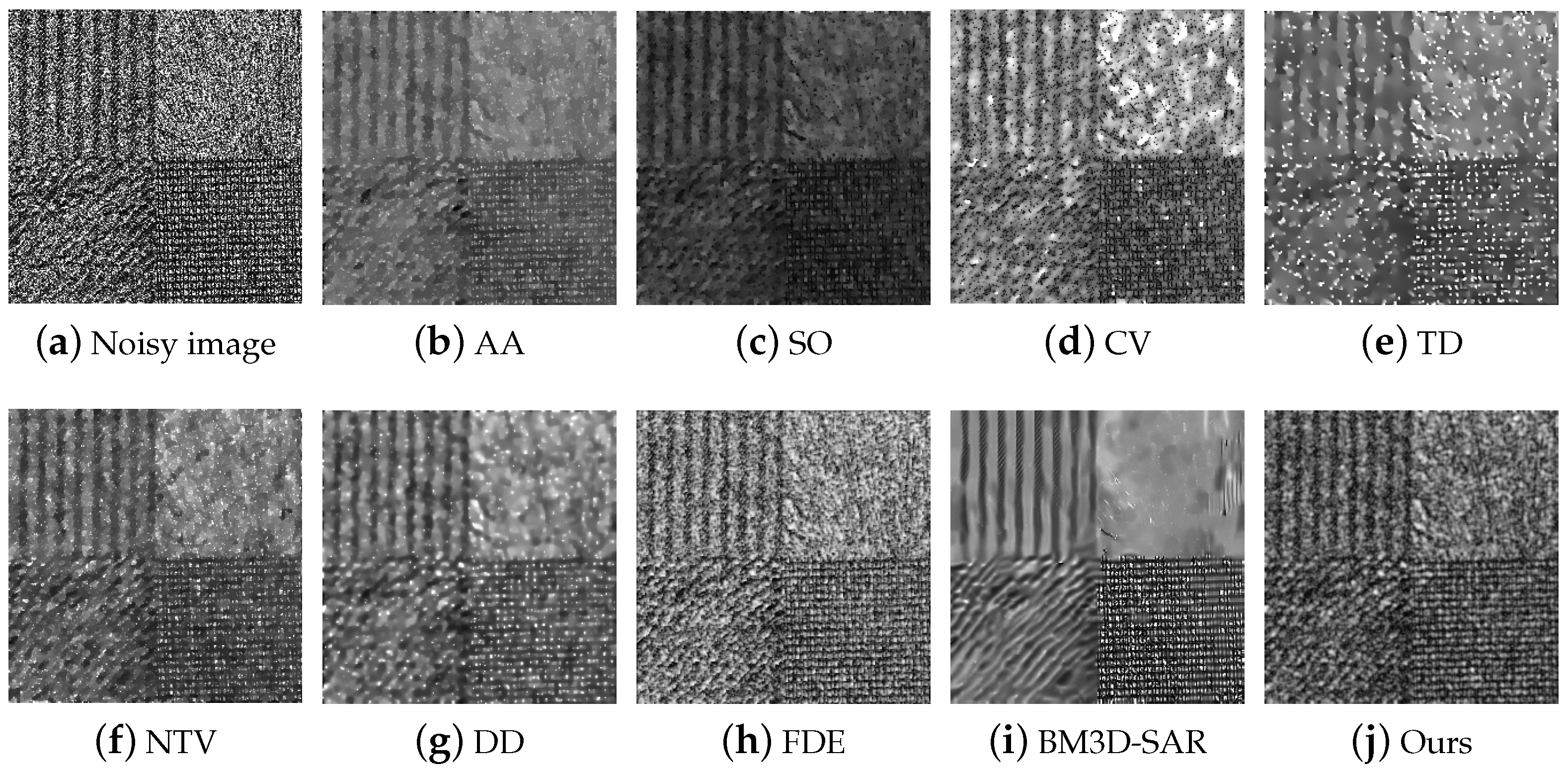
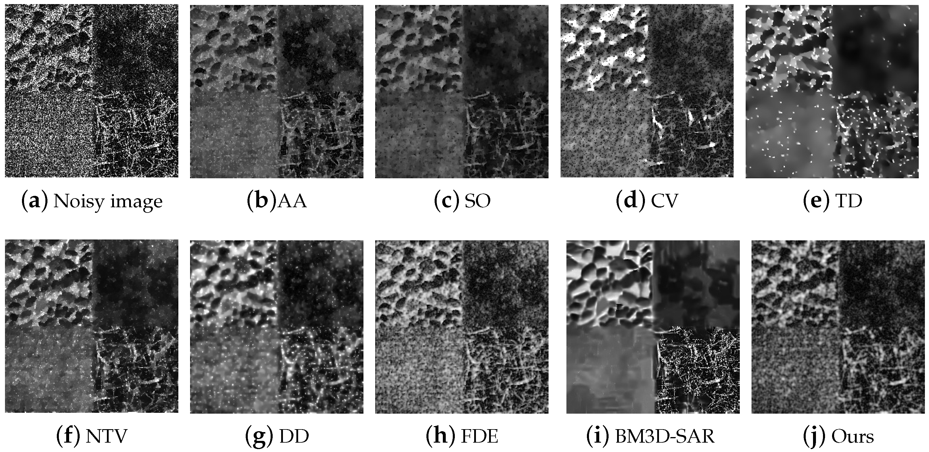
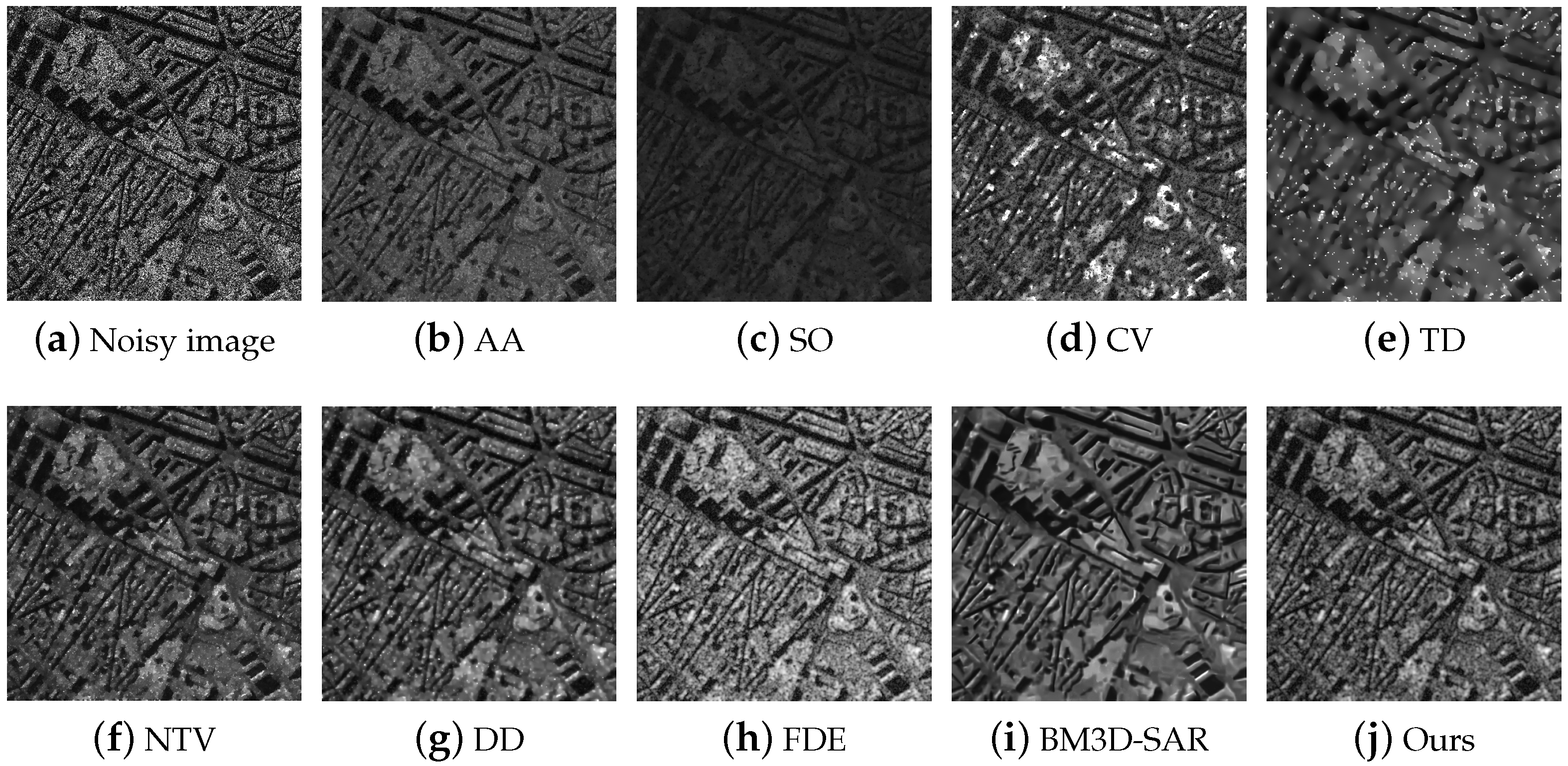
To demonstrate the despeckling ability of the FTDE method, various experiments are carried out applying different test images which are degraded by multiplicative noise with the looks $L=1,4,10$. In Figure 2, we show the original test images used in the numerical simulations. We display the restored results of four test images contaminated by multiplicative noise with $L=1$ in Figure 3, Figure 4, Figure 5 and Figure 6. For the quantitative comparison, we present the PSNR, MAE, SSIM, and IICC values of the despeckled results in

Table 3. Quantitative comparison of the different models for the texture1 image.

Model	SO	CV	AA	TD	NTV	DD	FDE	BM3D-SAR	Ours
$L=1$
PSNR	9.31	10.98	12.65	11.15	12.45	12.57	12.58	12.83	12.82
MAE	68.50	49.91	46.68	52.57	46.39	47.55	46.18	41.63	45.56
SSIM	0.15	0.31	0.25	0.21	0.31	0.25	0.40	0.36	0.40
IICC	0.52	0.43	0.54	0.38	0.53	0.46	0.58	0.59	0.55
$L=4$
PSNR	14.65	13.73	13.90	13.87	15.27	14.55	15.78	15.85	15.70
MAE	34.81	39.11	41.75	38.42	32.15	36.66	31.62	29.31	32.22
SSIM	0.57	0.45	0.37	0.40	0.63	0.56	0.69	0.67	0.68
IICC	0.76	0.65	0.76	0.64	0.79	0.71	0.80	0.81	0.79
$L=10$
PSNR	17.13	15.28	14.80	16.56	17.85	17.27	18.22	18.30	18.07
MAE	25.98	33.09	37.54	27.30	23.41	26.28	23.48	21.81	24.14
SSIM	0.73	0.59	0.48	0.63	0.80	0.77	0.82	0.82	0.81
IICC	0.86	0.75	0.84	0.80	0.88	0.86	0.89	0.89	0.88

,

Table 4. Quantitative comparison of the different models for the texture2 image.

Model	SO	CV	AA	TD	NTV	DD	FDE	BM3D-SAR	Ours
$L=1$
PSNR	10.96	12.56	14.35	13.92	14.92	15.30	15.01	14.19	15.52
MAE	50.46	37.44	33.56	34.81	30.41	30.97	32.30	29.02	30.96
SSIM	0.23	0.37	0.39	0.29	0.37	0.39	0.43	0.43	0.45
IICC	0.72	0.62	0.75	0.64	0.74	0.74	0.76	0.71	0.76
$L=4$
PSNR	17.66	16.55	15.38	16.61	17.99	17.56	18.06	17.47	18.17
MAE	22.10	25.84	31.45	24.85	20.91	23.18	22.58	21.14	22.53
SSIM	0.60	0.49	0.51	0.51	0.63	0.64	0.67	0.62	0.68
IICC	0.87	0.82	0.87	0.82	0.88	0.85	0.88	0.86	0.88
$L=10$
PSNR	19.80	18.28	15.74	19.07	20.45	20.04	20.62	20.22	20.48
MAE	16.97	20.76	30.43	18.52	15.62	17.23	16.56	15.64	16.87
SSIM	0.75	0.65	0.56	0.70	0.80	0.79	0.80	0.79	0.80
IICC	0.92	0.88	0.91	0.90	0.93	0.92	0.93	0.93	0.93

,

Table 5. Quantitative comparison of the different models for the satellite1 image.

Model	SO	CV	AA	TD	NTV	DD	FDE	BM3D-SAR	Ours
$L=1$
PSNR	13.02	15.44	17.77	17.47	18.56	20.26	19.61	20.50	20.47
MAE	42.07	25.80	23.09	22.33	20.57	17.75	18.84	16.55	17.46
SSIM	0.28	0.36	0.64	0.46	0.46	0.73	0.73	0.74	0.76
IICC	0.82	0.67	0.79	0.68	0.81	0.85	0.85	0.86	0.86
$L=4$
PSNR	20.64	21.75	21.20	21.40	21.67	22.60	22.89	23.40	23.18
MAE	16.15	14.59	15.39	14.31	14.15	13.13	12.94	11.59	12.58
SSIM	0.78	0.60	0.86	0.80	0.66	0.86	0.88	0.88	0.88
IICC	0.90	0.90	0.90	0.88	0.90	0.92	0.92	0.93	0.93
$L=10$
PSNR	23.62	24.04	23.96	23.93	23.74	24.64	24.97	25.66	25.19
MAE	11.33	11.03	11.05	10.74	11.17	10.30	10.17	8.93	9.91
SSIM	0.89	0.90	0.92	0.92	0.93	0.93	0.93	0.94	0.93
IICC	0.94	0.94	0.95	0.94	0.94	0.95	0.95	0.96	0.95

and

Table 6. Quantitative comparison of the different models for the satellite2 image.

Model	SO	CV	AA	TD	NTV	DD	FDE	BM3D-SAR	Ours
$L=1$
PSNR	11.03	13.74	16.32	15.38	16.52	17.74	16.33	17.90	17.77
MAE	56.07	34.88	29.43	29.66	27.68	24.94	29.29	23.77	24.97
SSIM	0.28	0.25	0.53	0.48	0.32	0.59	0.58	0.61	0.61
IICC	0.78	0.65	0.79	0.68	0.78	0.81	0.78	0.82	0.81
$L=4$
PSNR	18.68	18.90	17.43	18.76	19.18	19.53	19.67	20.07	19.90
MAE	21.80	21.23	26.48	20.93	20.20	29.71	19.85	18.33	19.42
SSIM	0.75	0.44	0.65	0.73	0.54	0.77	0.78	0.80	0.79
IICC	0.88	0.86	0.88	0.85	0.88	0.88	0.89	0.89	0.89
$L=10$
PSNR	21.07	20.65	17.86	20.88	21.10	21.34	21.60	21.92	21.72
MAE	16.32	17.17	25.37	16.59	16.13	16.04	15.85	14.80	15.68
SSIM	0.87	0.82	0.69	0.85	0.88	0.86	0.87	0.88	0.87
IICC	0.92	0.91	0.91	0.91	0.92	0.92	0.93	0.93	0.93

, where the best test results are shown in bold face.

From the visual quality of Figure 3, Figure 4, Figure 5 and Figure 6, it is easy to see that our FTDE model gives better test results in terms of multiplicative noise removal than the other compared methods. The common drawback of the SO algorithm, the CV algorithm, the TD algorithm, the AA algorithm, and the NTV algorithm, is excessive smoothness, resulting in the finer details of the original images may not be recovered satisfactorily. As we know, the DD method is based on the nonlinear diffusion equation framework, which can obtain better performance than TV-based methods. However, we can observe that the DD method retained isolated white speckle points in Figure 3g, Figure 4g, Figure 5g and Figure 6g. It is easy to find that the despeckled output obtained from the DD model is not very successful, because the difference operator in this algorithm is local. The FDE algorithm can preserve part of the texture details, but it is not satisfactory enough. Figure 3i, Figure 4i, Figure 5i and Figure 6i show that the BM3D-SAR method is effective in denoising texture images corrupted by multiplicative noise; however, this method causes artificial effects due to the stacking of image blocks in the BM3D-SAR method. For example, some artificial edges and textures appear at the top right part of satellite2 image. In terms of visual effects, the BM3D-SAR method is excessively smooth for some texture details. Since textures are similar to noise, the BM3D-SAR method may remove some textures as noise, and this method will result in incorrect texture information. In contrast, our method is proposed in a combined fractional-order derivative and telegraph diffusion equation framework, which effectively removes multiplicative noise and protect some texture structures, see Figure 3j, Figure 4j, Figure 5j and Figure 6j. In addition, our model does not cause artificial effects. There is little difference in quantitative evaluation between our method and the state of the art method, while our method is more real than the BM3D-SAR method in terms of denoising effect for texture images.

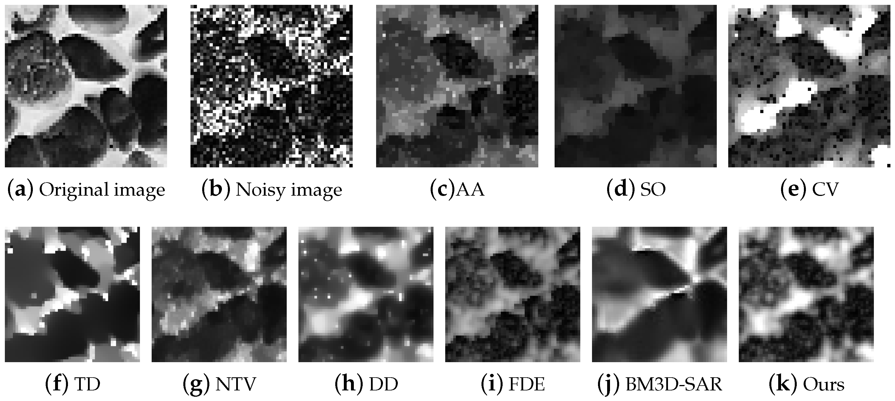
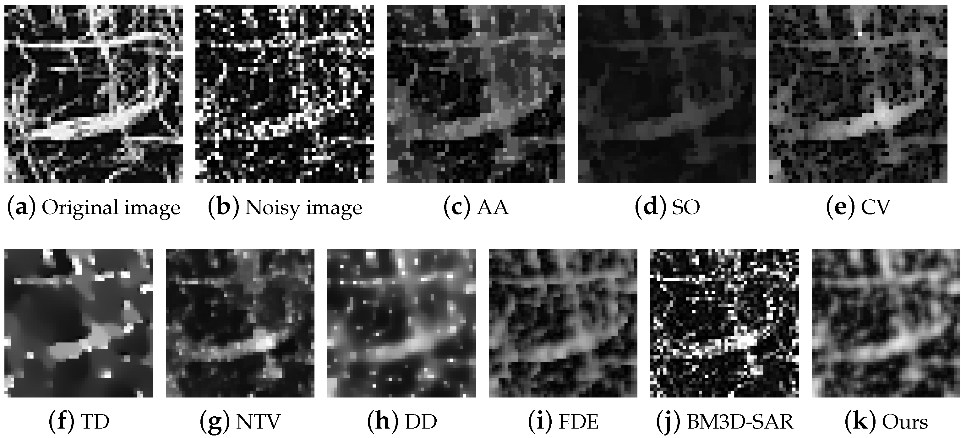
For a clear comparison, we present the zoomed details of the texture1 image obtained by different denoising models in Figure 7 and Figure 8. We choose two parts of the texture1 image that contain plenty of fine detail information. Compared to other methods, our method does a better job preserving textures.

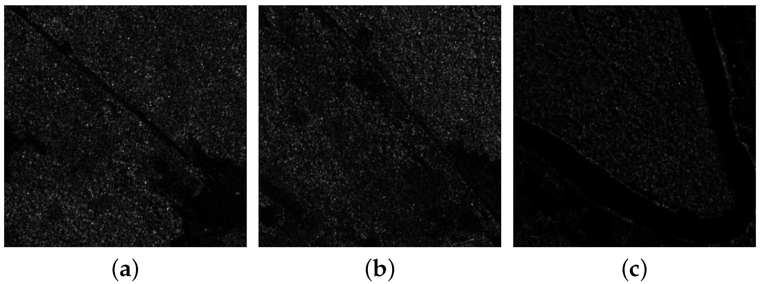
We not only denoise the artificial noise image but also recover the real SAR image. We show three real SAR images in Figure 9, and we display the corresponding denoising results obtained by using the FTDE model in Figure 10. In the simulations, we set $\lambda =0.1$ for three images, $b=2$ and $\epsilon =3\times {10}^{-7}$ for Figure 10a, $b=2.5$ and $\epsilon ={10}^{-7}$ for Figure 10b, $b=2$ and $\epsilon ={10}^{-7}$ for Figure 10c. Observing the result in Figure 10, one can find that the corresponding results may be well despeckled with efficient shape. Moreover, our model can preserve the details and edges of the real SAR images. Therefore, it is easy to say that the proposed algorithm is promising and robust for the speckle noise removal problem in SAR images.

6. Conclusions

In this paper, we proposed a fractional-order telegraph diffusion equation with the gray level indicator to remove the multiplicative noise from texture images. By combining the advantages of the fractional-order derivative and telegraph diffusion equation, the FTDE model features dual preservation for some textures. Due to the introduction of the gray level indicator in the diffusion coefficient, the FTDE model is beneficial to remove high level noise and preserve structural details. We proved the existence and uniqueness of the weak solution of the presented model and provided a numerical algorithm in the frequency domain. Numerical results show that our model is able to preserve structural details of texture images while removing multiplicative noise, both in terms of visual effects and quantitative analysis. They also show the potential of the fractional-order derivative operator in further image processing tasks. However, the internal essential mechanism of the fractional-order derivative and textures in our model is not clear enough. In future work, we will delve into the essential connection between fractional order derivatives and texture images.

References

1. Tur, M.; Chin, K.; Goodman, J. When is speckle noise multiplicative? Appl. Opt. 1982, 21, 1157–1159. [Google Scholar] [CrossRef] [PubMed]
2. Wagner, R.; Smith, S.; Sandrik, J.; Lopez, H. Statistics of speckle in ultrasound B-scans. IEEE Trans. Son. Ultrason. 1983, 30, 156–163. [Google Scholar] [CrossRef]
3. Argenti, F.; Lapini, A.; Bianchi, T.; Alparone, L. A tutorial on speckle reduction in synthetic aperture radar images. IEEE Geosci. Remote Sens. Mag. 2013, 1, 6–35. [Google Scholar] [CrossRef] [Green Version]
4. Yao, W.; Guo, Z.; Sun, J.; Wu, B.; Gao, H. Multiplicative noise removal for texture images based on adaptive anisotropic fractional diffusion equations. SIAM J. Imaging Sci. 2019, 12, 839–873. [Google Scholar] [CrossRef]
5. Majee, S.; Ray, R.; Majee, A. A gray level indicator-based regularized telegraph diffusion model: Application to image despeckling. SIAM J. Imaging Sci. 2020, 13, 844–870. [Google Scholar] [CrossRef]
6. Bamler, R. Principles of synthetic aperture radar. Surv. Geophys. 2000, 21, 147–157. [Google Scholar] [CrossRef]
7. Oliver, C.; Quegan, S. Understanding Synthetic Aperture Radar Images; SciTech Publishing: Raleigh, NC, USA, 2004. [Google Scholar]
8. Aubert, G.; Aujol, J. A variational approach to removing multiplicative noise. SIAM J. Appl. Math. 2008, 68, 925–946. [Google Scholar] [CrossRef]
9. Shi, J.; Osher, S. A nonlinear inverse scale space method for a convex multiplicative noise model. SIAM J. Imaging Sci. 2008, 1, 294–321. [Google Scholar] [CrossRef]
10. Huang, Y.; Ng, M.; Wen, Y. A new total variation method for multiplicative noise removal. SIAM J. Imaging Sci. 2009, 2, 20–40. [Google Scholar] [CrossRef] [Green Version]
11. Dong, Y.; Zeng, T. A convex variational model for restoring blurred images with multiplicative noise. SIAM J. Imaging Sci. 2013, 6, 1598–1625. [Google Scholar] [CrossRef]
12. Abd-Elmoniem, K.; Youssef, A.; Kadah, Y. Real-time speckle reduction and coherence enhancement in ultrasound imaging via nonlinear anisotropic diffusion. IEEE Trans. Biomed. Eng. 2002, 49, 997–1014. [Google Scholar] [CrossRef] [PubMed]
13. Zhou, Z.; Guo, Z.; Dong, G.; Sun, J.; Zhang, D.; Wu, B. A doubly degenerate diffusion model based on the gray level indicator for multiplicative noise removal. IEEE Trans. Image Process. 2015, 24, 249–260. [Google Scholar] [CrossRef] [PubMed]
14. Averbuch, A.; Epstein, B.; Rabin, N.; Turkel, E. Edge-enhancement postprocessing using artificial dissipation. IEEE Trans. Image Process. 2006, 15, 1486–1498. [Google Scholar] [CrossRef] [PubMed]
15. Ratner, V.; Zeevi, Y. Image enhancement using elastic manifolds. In Proceedings of the 14th International Conference on Image Analysis and Processing, Modena, Italy, 10–14 September 2007; pp. 769–774. [Google Scholar]
16. Zauderer, E. Partial Differential Equations of Applied Mathematics; John Wiley & Sons: New York, NY, USA, 2011. [Google Scholar]
17. Cao, Y.; Yin, J.; Liu, Q.; Li, M. A class of nonlinear parabolic-hyperbolic equations applied to image restoration. Nonlinear Anal. Real World Appl. 2010, 11, 253–261. [Google Scholar] [CrossRef]
18. You, Y.; Kaveh, M. Fourth-order partial differential equations for noise removal. IEEE Trans. Image Process. 2000, 9, 1723–1730. [Google Scholar] [CrossRef] [Green Version]
19. Zeng, W.; Lu, X.; Tan, X. A class of fourth-order telegraph-diffusion equations for image restoration. J. Appl. Math. 2011, 2011, 240370. [Google Scholar] [CrossRef] [Green Version]
20. Zhang, W.; Li, J.; Yang, Y. Spatial fractional telegraph equation for image structure preserving denoising. Signal Process. 2015, 107, 368–377. [Google Scholar] [CrossRef]
21. Majee, S.; Jain, S.K.; Ray, R.K.; Majee, A.K. A Fuzzy Edge Detector Driven Telegraph Total Variation Model for Image Despeckling. arXiv 2019. [Google Scholar] [CrossRef]
22. Shymanskyi, V.; Sokolovskyy, Y. Variational Formulation of the Stress-Strain Problem in Capillary-Porous Materials with Fractal Structure. In Proceedings of the IEEE 15th International Conference on Computer Sciences and Information Technologies (CSIT), Zbarazh, Ukraine, 23–26 September 2020; pp. 1–4. [Google Scholar]
23. Hendy, M.; Amin, M.; Ezzat, M. Two-dimensional problem for thermoviscoelastic materials with fractional order heat transfer. J. Therm. Stress. 2019, 42, 1298–1315. [Google Scholar] [CrossRef]
24. Zhou, J.; Salahshour, S.; Ahmadian, A. Modeling the dynamics of COVID-19 using fractal-fractional operator with a case study. Results Phys. 2022, 33, 105103. [Google Scholar] [CrossRef]
25. Bai, J.; Feng, X. Fractional-order anisotropic diffusion for image denoising. IEEE Trans. Image Process. 2007, 16, 2492–2502. [Google Scholar] [CrossRef]
26. Cuesta, E.; Finat, J. Image Processing by means of linear integro-differential equation. In Proceedings of the Third IASTED International Conference on Visualization, Imaging and Image Processing, Benalmadena, Spain, 8–10 September 2003. [Google Scholar]
27. Janev, M.; Pilipović, S.; Atanacković, T.; Obradović, R.; Ralević, N. Fully fractional anisotropic diffusion for image denoising. Math. Comput. Model. 2011, 54, 729–741. [Google Scholar] [CrossRef]
28. Zhang, J.; Chen, K. A total fractional-order variation model for image restoration with nonhomogeneous boundary conditions and its numerical solution. SIAM J. Imaging Sci. 2015, 8, 2487–2518. [Google Scholar] [CrossRef] [Green Version]
29. Zhang, J.; Wei, Z.; Xiao, L. A fast adaptive reweighted residual-feedback iterative algorithm for fractional-order total variation regularized multiplicative noise removal of partly-textured images. Signal Process. 2014, 98, 381–395. [Google Scholar] [CrossRef]
30. Chen, D.; Sun, S.; Zhang, C.; Chen, Y.; Xue, D. Fractional-order TV-L2 model for image denoising. Open Phys. 2013, 11, 1414–1422. [Google Scholar] [CrossRef] [Green Version]
31. Dong, F.; Chen, Y. A fractional-order derivative based variational framework for image denoising. Inverse Probl. Imaging 2016, 10, 27–50. [Google Scholar] [CrossRef] [Green Version]
32. Che, J.; Guan, Q.; Wang, X. Image denoising based on adaptive fractional partial differential equations. In Proceedings of the 2013 6th International Congress on Image and Signal Processing (CISP), Hangzhou, China, 16–18 December 2013; pp. 288–292. [Google Scholar]
33. Pu, Y. Fractional calculus approach to texture of digital image. In Proceedings of the International Conference on Signal Processing, Guilin, China, 16–20 November 2006; pp. 1002–1006. [Google Scholar]
34. Pu, Y.; Wang, W.; Zhou, J.; Wang, Y.; Jia, H. Fractional differential approach to detecting textural features of digital image and its fractional differential filter implementation. Sci. China 2008, 51, 1319–1339. [Google Scholar] [CrossRef]
35. Zhang, X.; Liu, R.; Ren, J.; Gui, Q. Adaptive Fractional Image Enhancement Algorithm Based on Rough Set and Particle Swarm Optimization. Fractal Fract. 2022, 6, 100. [Google Scholar] [CrossRef]
36. Li, D.; Tian, X.; Jin, Q.; Hirasawa, K. Adaptive fractional-order total variation image restoration with split Bregman iteration. ISA Trans. 2017, 82, 210–222. [Google Scholar] [CrossRef] [PubMed]
37. Shan, X.; Sun, J.; Guo, Z.; Yao, W.; Zhou, Z. Fractional-order diffusion model for multiplicative noise removal in texture-rich images and its fast explicit diffusion solving. BIT Numer. Math. 2022, 62, 1319–1354. [Google Scholar] [CrossRef]
38. Ju, N. The maximum principle and the global attractor for the dissipative 2D quasi-geostrophic equations. Commun. Math. Phys. 2005, 255, 161–181. [Google Scholar] [CrossRef]
39. Burczak, J.; Granero-Belinchón, R. Suppression of blow up by a logistic source in 2D Keller–Segel system with fractional dissipation. J. Differ. Equ. 2017, 263, 6115–6142. [Google Scholar] [CrossRef] [Green Version]
40. Schumer, R.; Benson, D.; Meerschaert, M.; Wheatcraft, S. Eulerian derivation of the fractional advection-dispersion equation. J. Contam. Hydrol. 2001, 48, 69–88. [Google Scholar] [CrossRef]
41. He, J. Approximate analytical solution for seepage flow with fractional derivatives in porous media. Comput. Methods Appl. Mech. Eng. 1998, 167, 57–68. [Google Scholar] [CrossRef]
42. Chen, S.; Liu, F.; Jiang, X.; Turner, I.; Burrage, K. Fast finite difference approximation for identifying parameters in a two-dimensional space-fractional nonlocal model with variable diffusivity coefficients. SIAM J. Numer. Anal. 2017, 54, 606–624. [Google Scholar] [CrossRef]
43. Pan, M.; Zheng, L.; Liu, F.; Liu, C.; Chen, X. A spatial-fractional thermal transport model for nanofluid in porous media. Appl. Math. Model. 2018, 53, 622–634. [Google Scholar] [CrossRef]
44. Podlubny, I. Fractional Differential Equations, an Introduction to Fractional Derivatives, Fractional Differential Equations, to Methods of Their Solution and Some of Their Applications; Mathematics in Science and Engineering Process; Mag. Academic Press: San Diego, CA, USA, 1999. [Google Scholar]
45. Xu, W.; Tang, C.; Zhang, J.; Su, Y.; Su, R.K.L. Two parabolic–hyperbolic oriented partial differential equations for denoising in electronic speckle pattern interferometry fringes. Appl. Opt. 2015, 54, 4720–4726. [Google Scholar] [CrossRef]
46. Zhou, Z.; Guo, Z.; Zhang, D.; Wu, B. A nonlinear diffusion equation-based model for ultrasound speckle noise removal. J. Nonlinear Sci. 2018, 28, 443–470. [Google Scholar] [CrossRef]
47. Shan, X.; Sun, J.; Guo, Z. Multiplicative noise removal based on the smooth diffusion equation. J. Math. Imaging Vis. 2019, 61, 763–779. [Google Scholar] [CrossRef]
48. Tychonoff, A. Ein fixpunktsatz. Math. Ann. 1935, 111, 767–776. [Google Scholar] [CrossRef]
49. Adams, R.; Fournier, J. Sobolev Spaces; Elsevier: Amsterdam, The Netherlands, 2003. [Google Scholar]
50. Evans, L. Partial Differential Equations; American Mathematical Society: Providence, RI, USA, 2010. [Google Scholar]
51. Lions, J.; Magenes, E. Non-Homogeneous Boundary Value Problems and Applications; Springer Science & Business Media: Berlin/Heidelberg, Germany, 2012. [Google Scholar]
52. Roubíček, T. Nonlinear Partial Differential Equations with Applications; Springer Science & Business Media: Berlin/Heidelberg, Germany, 2013. [Google Scholar]
53. Candan, C.; Kutay, M.; Ozaktas, H. The discrete fractional Fourier transform. In Proceedings of the IEEE International Conference on Acoustics, Speech, and Signal Processing, Phoenix, AZ, USA, 15–19 March 1999; pp. 1713–1716. [Google Scholar]
54. Ozaktas, H.; Arikan, O.; Kutay, M.; Bozdagt, G. Digital computation of the fractional Fourier transform. IEEE Trans. Signal Process. 1996, 44, 2141–2150. [Google Scholar] [CrossRef] [Green Version]
55. Taylor, M. Partial Differential Equations I; Basic Theory, Applied Mathematical Sciences; Springer: New York, NY, USA, 2011. [Google Scholar]
56. LeVeque, R. Finite Difference Methods for Ordinary and Partial Differential Equations: Steady-State and Time-Dependent Problems; Society for Industrial and Applied Mathematics: Philadelphia, PA, USA, 2007. [Google Scholar]
57. Do, M.; Vetterli, M. The finite ridgelet transform for image representation. IEEE Trans. Image Process. 2003, 12, 16–28. [Google Scholar] [CrossRef] [Green Version]
58. Deledalle, C.; Denis, L.; Tabti, S.; Tupin, F.; Reigber, A.; Jager, M. Mulog, or how to apply Gaussian denoisers to multi-channel SAR speckle reduction? IEEE Trans. Image Process. 2017, 26, 4389–4403. [Google Scholar] [CrossRef] [Green Version]
59. Durand, S.; Fadili, J.; Nikolova, M. Multiplicative noise removal using L1 fidelity on frame coefficients. J. Math. Imaging Vis. 2010, 36, 201–226. [Google Scholar] [CrossRef] [Green Version]
60. Wang, Z.; Bovik, A.; Sheikh, H.; Simoncelli, E. Image quality assessment: From error visibility to structural similarity. IEEE Trans. Image Process. 2004, 13, 600–612. [Google Scholar] [CrossRef]
61. Wang, Z.; Bovik, A.; Lu, L. Why is image quality assessment so difficult? In Proceedings of the IEEE International Conference on Acoustics, Speech, and Signal Processing, Hong Kong, China, 6–10 April 2003. [Google Scholar]
Figure 1. Comparison results: (a) Original signal. (b) Result of telegraph diffusion-based model. (c) Result of non-telegraph diffusion-based model.
Fractalfract 07 00064 g001
Figure 2. Test images. (a) Texture1. (b) Texture2. (c) Satellite1. (d) Satellite2.
Fractalfract 07 00064 g002
Figure 3. The despeckled results on the texture1 image: (a) Noisy: L = 1 . (bj) Despeckled results.
Fractalfract 07 00064 g003
Figure 4. The despeckled results on the texture2 image: (a) Noisy: L = 1 . (bj) Despeckled results.
Fractalfract 07 00064 g004
Figure 5. The despeckled results on the satellite1 image: (a) Noisy: L = 1 . (bj) Despeckled results.
Fractalfract 07 00064 g005
Figure 6. The despeckled results on the satellite2 image: (a) Noisy: L = 1 . (bj) Despeckled results.
Fractalfract 07 00064 g006
Figure 7. The first zoomed detail of despeckled results on the texture1 image: (a) The original image. (b) Noisy: L = 1 . (ck) Despeckled results.
Fractalfract 07 00064 g007
Figure 8. The second zoomed detail of despeckled results on the texture1 image: (a) The original image. (b) Noisy: L = 1 . (ck) Despeckled results.
Fractalfract 07 00064 g008
Figure 9. Real SAR images: (a) The SAR1 image. (b) The SAR2 image. (c) The SAR3 image.
Fractalfract 07 00064 g009
Figure 10. Restored real SAR images by the FTDE model: (a) The restored SAR1 image. (b) The restored SAR2 image. (c) The restored SAR3 image.
Fractalfract 07 00064 g010