Abstract
The multifractal relationship between reference evapotranspiration (ET0), computed by the Penmann-Monteith equation (PM), relative humidity () and mean surface temperature () was studied in the middle zone of the Guadalquivir River Valley (south Spain) in a previous study. This work extends that study to the average wind speed () and solar radiation (), focusing on more recent years. All agro-meteorological variables were analyzed by multifractal detrended cross-correlation analysis (MFCCA) and multifractal detrended fluctuation analysis (MFDFA). The outcomes revealed persistent long-term autocorrelations, with and having the highest persistence (). More precise results of multifractal properties than in the previous study were obtained for , , and due to the elimination of trends in the signals. Only medium and large fluctuations in showed multifractal cross-correlations with its controlling factors, except for . Moreover, joint scaling exponents differed from individual exponents. These phenomena contrast with what has been observed in previous cross-correlation studies, revealing that some differences exist in the dynamics of multifractality among the analyzed variables. On the other hand, the – relation showed that extreme events in are mainly ruled by high temperature fluctuations, which match conclusions drawn in the previous study.
1. Introduction
Evapotranspiration is an important variable for scheduling irrigation systems and water resource planning, which directly influence crop yield and are strongly dependent on climatic conditions [1]. This variable is the combination of two factors: water evaporation from the soil, ruled by climatic conditions, and crop evaporation and transpiration, which are governed both by physical and biological processes [2]. In 1975, the United Nations Food and Agriculture Organization (FAO) established a conventional computing technique to determine an approximation of actual evapotranspiration when measuring it using lysimeters and evaporation pans is not possible. It simply involves separating these two factors into two different variables: reference evapotranspiration () and crop coefficients [2,3,4]. The former variable describes maximum evapotranspiration based on a reference crop: a natural grass surface with some specific features [5]. The most frequently used computing methods are based on the Thornthwaite, Hargreaves and Penman-Monteith (PM) equations [6]. However, the superiority of the FAO-56 PM equation [3] over other equations has been demonstrated [7,8].
Reference evapotranspiration has been a widely studied variable in the last decades, including investigations of its temporal and spatial patterns related to the climate change [1,6,9,10,11] and its role in models of the phenological response of olive crops [12].
Different agro-meteorological variables (such as , surface temperature, and wind speed), are characterized by nonlinear characteristics which evolve differently at distinct timescales, showing a multifractal nature [13]. The multifractal theory states that some systems and, particularly, some time series might be described by a combination of mixed fractal subsets [14,15], each characterized by a different scaling exponent or singularity strength [2,16]. The variable has also nonlinear relationships with its controlling factors, which reveals multifractal cross-correlations, as has been shown in previous studies [17,18,19,20]. Therefore, the study of the nonlinearity and scaling properties of might be of help in improving the modelling of the interrelationships between these variables [17,20].
A common method for studying the multifractality of a nonlinear time series is multifractal detrended analysis (MFDFA), proposed by Kantelhardt et al. [21]. However, to analyze the multifractality of cross-correlations between two time series, multifractal detrended cross-correlation analysis (MFCCA) is increasingly being used [22,23,24]. This technique was proposed by Oświȩcimka et al. as a proper generalization of the computation of the fractal cross-correlation scaling exponent, , for different statistical moments to determine multifractal cross-correlations between two time series [25]. The exponent is based on the detrended fluctuation analysis (DCCA), which was first used by Podobnik and Stanley [26] to investigate power law correlations between different time series in the presence of nonstationarity. Additionally, it quantifies the strength of these cross-correlations for fluctuations of different sizes, identifying the main dominant fluctuations in the interaction between different variables [27].
In a preceding study, multifractal relations between and two of its predictor variables, mean temperature () and relative humidity (), were found in the area of the middle zone of the Guadalquivir River Valley (south Spain) by using joint multifractal analysis [2]. Despite the successful application of this methodology in different fields [28,29,30], it presents some difficulties when attempting to interpret more than three variables’ distributions [2]. For this reason, a study of correlations between and meteorological variables using a method whose results are more easily interpretable, such as MFCCA, is relevant for a better understanding of the interactions between these variables. This method has gained popularity in the study of in recent years [17,19]. Therefore, the aim of this study is to extend the research into the interaction of in the work of Ariza-Villaverde et al. [2] with the mentioned and , as well as the average wind speed at 2 m above the surface () and solar radiation (). For this purpose, an agro-meteorological time series of 21 years data (in the period 2001–2021) and daily resolution were selected to be analyzed. Individual multifractal exponents were also computed by MFDFA to compare them to the cross-correlation results.
2. Materials and Methods
2.1. Data
Daily records of mean temperature (), relative humidity (), wind speed at 2 m heigh (), and solar radiation () in the period 2001–2021 were used in this study (a total of data). Raw data from climatic variables had less than 1% missing values and were obtained from the Open Data website https://www.juntadeandalucia.es/agriculturaypesca/ifapa/riaweb/web/datosabiertos (accessed on 27 December 2022). Missing values were omitted in our calculations. The station is located in the city of Córdoba, southern Spain (37°51′25″ N, 4°48′10″ W; 94 m above sea level) and belongs to the Agroclimatic Information Network of Andalusia. The maintenance of this network and the cited website are carried out by the IFAPA (Andalusian Institute for Research and Training in Agriculture, Fishery, Food and Ecological Production) [31].
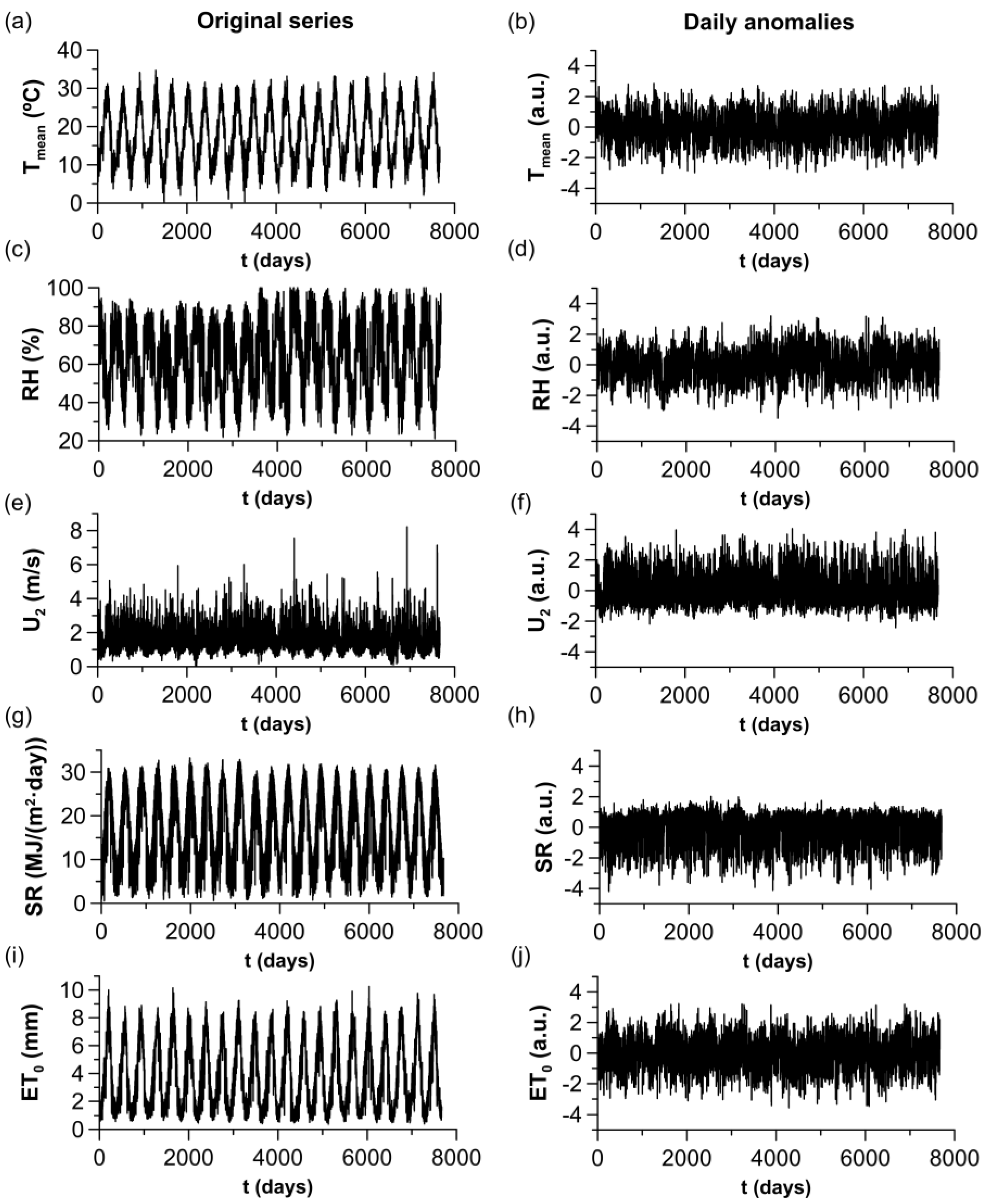
The area of study is characterized by a continental Mediterranean climate [32]: a temperate climate with dry and hot summers, classified as Csa according to the Köppen climate classification [2]. Reference evapotranspiration data from the same period were computed by the IFAPA from the climatic variables according to the FAO-56 Penman-Monteith (PM) equation [3]. All data series can be seen in Figure 1 and the main descriptive statistical parameters can be found in Table 1.
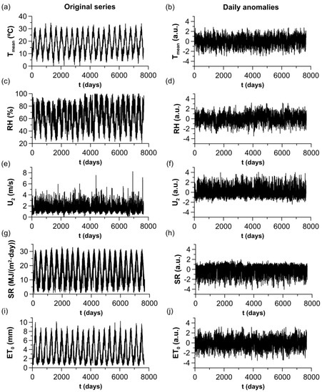
Figure 1.
Meteorological time series and reference evapotranspiration. (a,c,e,g,i) Original series. (b,d,f,h,j) Daily anomalies of time series. (a,b) Mean temperature (). (c,d) Relative humidity (). (e,f) Wind speed at 2 m heigh (). (g,h) Solar radiation (). (i,j) Reference evapotranspiration ().

Table 1.
Statistical properties of the agro-meteorological time series.
2.2. Seasonal Detrending
The agro-meteorological time series display seasonal trends (see Figure 1). Because periodicities can influence the analysis of nonlinear properties of time series [17,33], the seasonal component of these series must be eliminated before applying multifractal methods. For this purpose, the standardized anomalies of daily series were obtained using the following formula [16,34,35,36,37]: , where is the calendar mean and is the calendar standard deviation.
2.3. Multifractal Detrending Analysis Algorithms
The MFCCA and MFDFA algorithms are closely related. The former is based in DCCA and was conceived by Oświȩcimka et al. [25] to study the multifractal cross-correlations between two time series. The MFDFA method was developed by Kantelhardt et al. [21] as a generalization of the detrended fluctuation analysis [38] to obtain the scaling properties of one single multifractal stationary or nonstationary signal. Both consists of the following initial steps.
First, the integrated series after subtracting the mean or “profile” is computed in MFDFA (MFCCA) for the (two) time series ( and ), with :
Next, the profile is divided (both profiles are divided) into nonoverlapping segments of length , where denotes the greatest integer number lower than the quotient. The segments, , must be taken in both directions [19] to avoid the omission of the remaining part of the series in the calculations.
Then, for each one of segments, the local trend of the profile (each profile) is obtained by fitting a polynomial of order m (, ). Trends are subtracted from the series and the detrended cross-covariance (detrended variance) can be computed as:
for and
for .
It must be pointed out that the detrended variance is recovered in the MFDFA method by setting in Equations (2) and (3) [21]. Next, the average is computed over all segments for different q statistical moments and is repeated for different values of the length or scale, .
For the MFDFA method, the fluctuation function is obtained as:
For , the expression in Equation (4) diverges and a logarithmic averaging operation must be applied instead.
If the analyzed signal has long-range power law-correlated fluctuations, the fluctuation function can be expressed as:
The scaling exponent, , can be computed by the least-squares regression of versus in a log–log plot and is called the generalized Hurst exponent [39]. In fact, coincides with the value of the well-known classical Hurst exponent [39,40] for stationary series, whereas for nonstationary series the Hurst exponent is obtained from [16]. For positive values of , describes the scaling behavior of the large fluctuations whereas for negative it is related to the scaling behavior of the small fluctuations.
From , other interesting exponents can be derived [19]. The singularity exponent, , and its spectrum, , were considered relevant for this study since their results are widely used to assess the complexity of the studied signals [16,41,42,43,44,45]. The singularity exponent or Lipschitz-Hölder exponent, can be obtained as:
where is the mass exponent and can be computed from the expression [21]. Then, the singularity spectrum or multifractal spectrum can be computed by means of the Legendre transformation:
Plots of commonly have the shape of a concave down parabola with different properties which characterize them: the singularity of maximum spectrum, , the width, , and the asymmetry of the spectrum. The first property correspond to the most dominant scaling behavior, while the width indicates the strength of the multifractality of the signal [43]. Asymmetry is measured in different ways in the literature [41,43,46]. Here, the asymmetry index (AI) was used, in a similar manner as previous in studies of reference evapotranspiration [17,19]:
where and are, respectively, the widths of the left and right tails of the spectrum. Positive values of the AI describe left-skewed spectra, i.e., the left tail is wider than the right one [47]. These signals are characterized by more complex extreme events or large fluctuations and more regular and frequent small fluctuations. The opposite happens with negative values of the AI (right-skewed spectra), where spectra exhibit small fluctuations with fine structure. If the AI is zero, the spectrum is symmetric and the complexity of small fluctuations is similar to large fluctuations.
The cross-covariance obtained in MFCCA, unlike the detrended variance, can be positive or negative [25], and the qth-order covariance function is computed regarding the sign:
where denotes the sign function.
In this case, if both series are long term power-law cross-correlated, the covariance function is expected to exhibit the following relation:
where if the qth-order covariance function is negative and is the multifractal cross-correlation exponent and describes the fractal properties of the cross-covariance [25]. Note that Equation (10) is similar to Equation (5) in the MFDFA method. For monofractal cross-correlation, is independent of and has the same value obtained by DCCA [26]. For multifractal cross-correlation, the value computed by DCCA is equal to the multifractal exponent for the second statistical moment, .
Kwapień et al. defined the q-dependent detrended cross-correlation coefficient as the ratio between the detrended covariance () and variance () functions [27]:
For , the definition of the standard detrended cross-correlation coefficient () is retrieved [48]. However, the definition of a q-dependent coefficient allows the characterization of the cross-correlation of large and small fluctuations between both series for statistical moments which are higher or lower than 2, respectively [27]. For , values of this coefficient are bound within the same range as : . For negative moments, the computation of can lead to very large absolute values that deviate greatly from 1 due to very small values in the denominator in Equation (11). According to Kwapień et al. [27], this issue might be addressed by applying the multiplicative inverse of those values higher than the unit and the result, , is then within the range . If the signal fluctuations (for ) are weakly cross-correlated or are uncorrelated, values of this function either violently fluctuate within the interval or are close to zero. On the contrary, if small fluctuations are cross-correlated, a stable non-zero function is obtained for and some scales, even if the original values of the cross-correlation coefficients exceed 1 [27].
3. Results
3.1. MFDFA of Agro-Meteorological Times Series
MFDFA was applied to all four meteorological variables and , considering a range of scales, , between 8 and days, with steps of 1 day, and values of between −4 and 4, with steps of 0.2. These values are similar to those used in previous studies [2,13,17,19].
As Oświęcimka et al. state, the effects of trends in analyzed data is one of the problems that multifractal analysis has [49]. The polynomial of order two is most frequently used for detrending in MFDFA, however, this sometimes leads to less accurate results than using polynomials of higher orders, as the mentioned authors show. To investigate the optimum polynomial order, polynomial orders from up to 5 were chosen and the computation of the qth order detrended fluctuation functions were obtained in every case. Next, the polynomial order of trends for which the fluctuation functions better fitted to a power law (which yielded the highest Pearson correlation coefficients in the fits of the log–log plots) was chosen. We found that was the best order of the polynomial to perform the analysis.
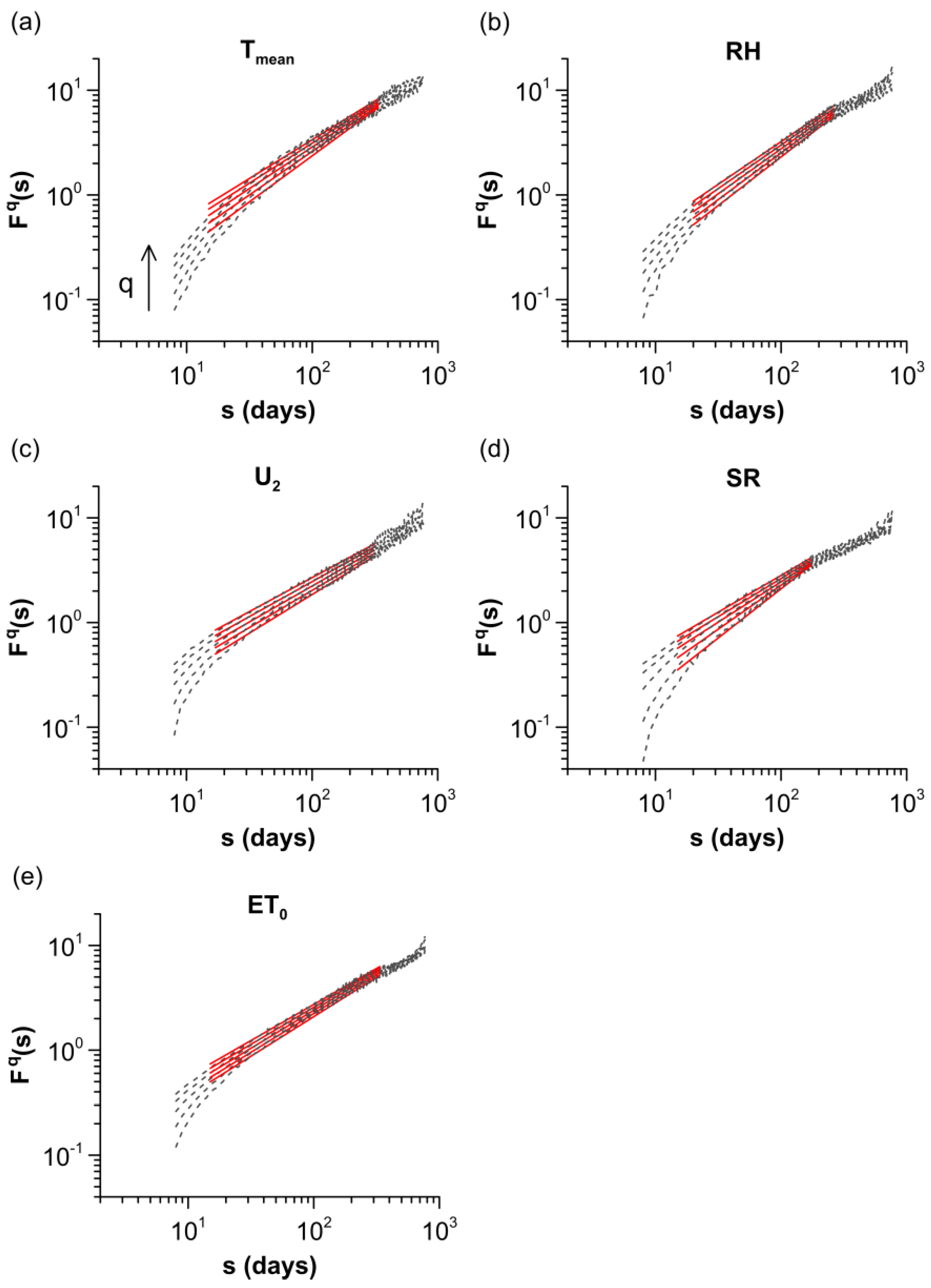
The fluctuation functions computed for the detrending polynomial order and are shown in Figure 2 for every agro-meteorological variable, and it can be seen that they are in increasing order of . The log–log plots of vs. the scale, fit well to a straight line for every moment and for a wide range of scales between 15–20 and 172–335 days. Fluctuation functions for every and all agro-meteorological variables show Pearson correlation coefficients that exceed the value of 0.990. According to the protocol of Makowiec and Fuliński [50], scaling exponents can be considered as representatives for the underlying scaling phenomena when a linear approximation for each in a logarithmic scale of the fluctuation function vs. dependence over the same range of scales has a Pearson correlation coefficient higher than 0.98.

Figure 2.
Detrended fluctuation functions (gray dashed lines) with their linear fits (red solid lines). For reasons of clarity, only fluctuation functions and their fits for are displayed. (a) . (b) . (c) . (d) . (e) .
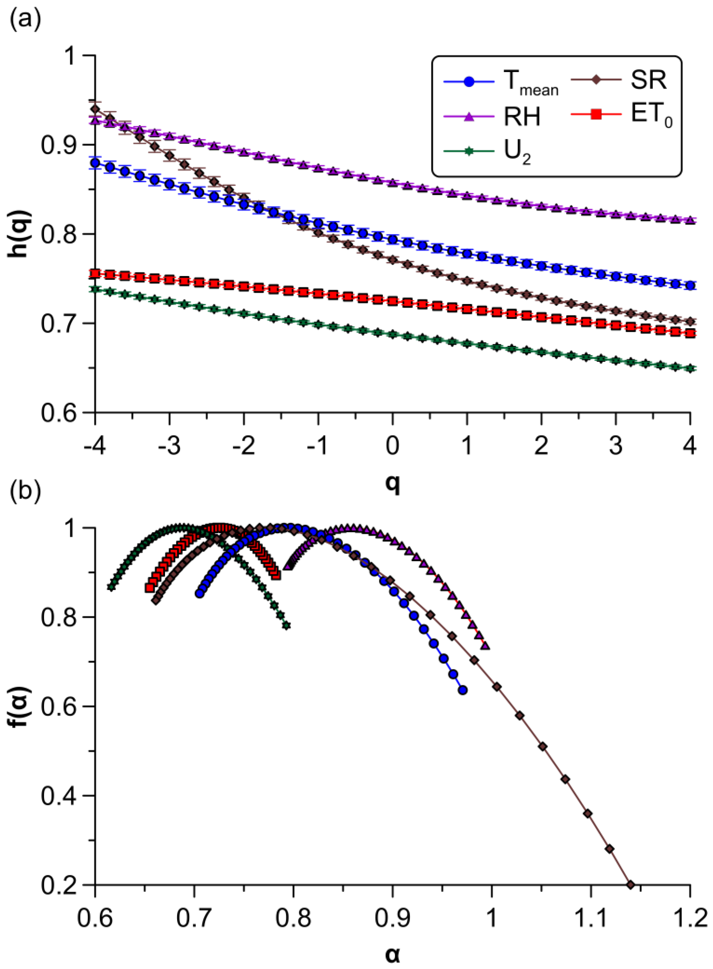
Generalized Hurst exponents or slopes from these fits with their statistical errors can be seen in Figure 3a. Since all the scaling exponents were higher than 0.5, small and large fluctuations of every variable displayed persistent long-range correlations. Similar outcomes have been obtained by other authors for the time series of daily maximum air temperature, minimum air temperature, and recorded in years 1992–2019 in India, and time series of daily air temperature, , , wind speed, air pressure, and recorded in the years 1961–1990 in California (USA) [17,19]. Moreover, different scaling exponents for every can be observed, which confirms their multifractal nature. The series exhibits the curve with the highest exponents for almost all the statistical moments considered, which means that this variable presents the most persistent correlations. For large and medium fluctuations, was followed in order of strength of correlations by , , and . For small and very small fluctuations, and both had the strongest correlations, followed by , and . This is due to the broad range of scaling exponents () that shows, approximately twice the value of the other variables (see Table 2). This denotes that the series exhibits the highest degree of multifractality and is the most complex signal.
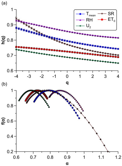
Figure 3.
Multifractal plots of agro-meteorogical variables. (a) Generalized Hurst exponents. (b) Multifractal spectra.

Table 2.
Multifractal parameters of the agro-meteorogical variables.
In Figure 3b, multifractal spectra of these variables are depicted. As can be seen in the figure, they are ordered from higher to lower value of (from right to left), where a lower value implies a less correlated signal (and one which has more complex small fluctuations). The width is much higher for the time series, again denoting a higher degree of multifractality for this variable. Additionally, the right tail of this spectrum indicates that small fluctuations of exhibit a fine structure which is characterized by the largest range of observed in these variables (see Table 2). Lastly, the AI suggests that all meteorological variables had slightly right-skewed spectra, where was noticeable by its clear asymmetric shape, whereas displayed an almost symmetric multifractal spectrum with a small deviation to a left-skewed spectrum. This means that the small fluctuations of the main controlling factors of had fine structure and were more complex, whereas those observed in reference evapotranspiration were more regular and homogeneous.
These outcomes differ considerably from those obtained by the joint multifractal analysis in the same area of study in the previous research [2]. Even though a higher number of years were analyzed here, different individual multifractal spectra for , and and their deviation from can explained due to the elimination of the trend component in MFDFA, which is known to affect the multifractal properties [33,49].
3.2. MFCCA of Meteorological Times Series with
Similarly, the MFCCA method was applied to pairs of meteorological factors and with the same range of moments and scales, used in the application of MFDFA. The same procedure explained in Section 3.1 was performed to find the optimum polynomial order of trends. Once again, the best order of polynomial to eliminate trends was observed to be .
Log–log plots of detrended cross-covariance functions for different values of are shown in Figure 4. It was found that the covariance function of and was negative, as might be expected, since a rise in one variable results in a reduction in the other and vice versa. For relatively high positive moments and several scales, covariance functions follow a power law. For negative and low positive moments, they are almost zero or display violent fluctuations around zero, with a sign which strongly depends on the timescale, leading to irregular curves like those shown in the figure. Consequently, meteorological variables do not show power law cross-correlations with for small fluctuations. Only the covariance between and also show a nonlinear scaling with violent fluctuations for and all scales (Figure 4c), denoting that neither variable exhibits multifractal cross-correlations.
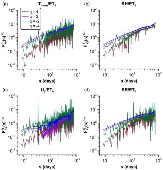
Figure 4.
Detrended cross-covariance functions . For reasons of clarity, only fluctuation functions for q = [4, 2, 2, 4] are displayed. (a) –. (b) –. (c) –. (d) –.
The existence of power-law cross-correlations between pairs of these meteorological factors and reference evapotranspiration have also been observed in previous studies [17,19]. However, in those studies they were observed for fluctuations of any magnitude. In this study, we have established that only large and medium fluctuations exhibit power-law temporal correlations, whereas correlations between small fluctuations do not follow Equation (10) or are negligible (see Figure 4). A similar behavior was found for several time series in a financial context [23,25,47].
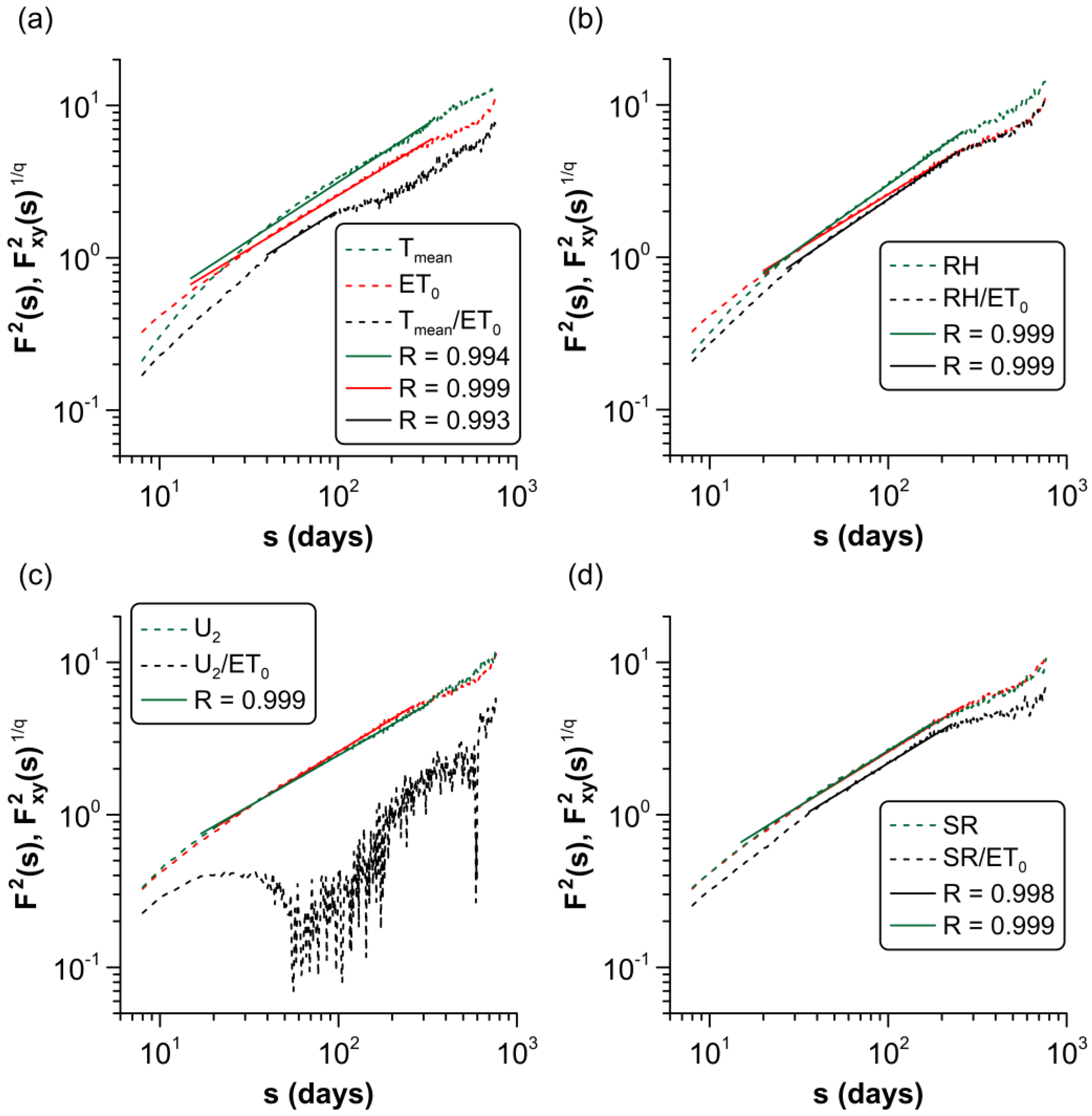
Log–log plots of the second-order covariance functions, , of each meteorological factor with and second-order variance functions, , obtained in the previous section, are shown together vs. the scale in Figure 5. Linear trends (solid lines) of and with scale can be noticed in Figure 5a,b,d, showing the power-law scaling of these functions. Correlation coefficients of linear fits for these curves can also be seen in this figure. Once again, the protocol of Makowiec and Fuliński was applied to the detrended cross-correlation functions to consider the scaling exponents as representatives of the scaling phenomenon [50].
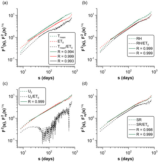
Figure 5.
Detrended variance and covariance functions for of meteorological variables with (dashed lines) and their linear fits (solid lines). (a) –. (b) –. (c) –. (d) –.
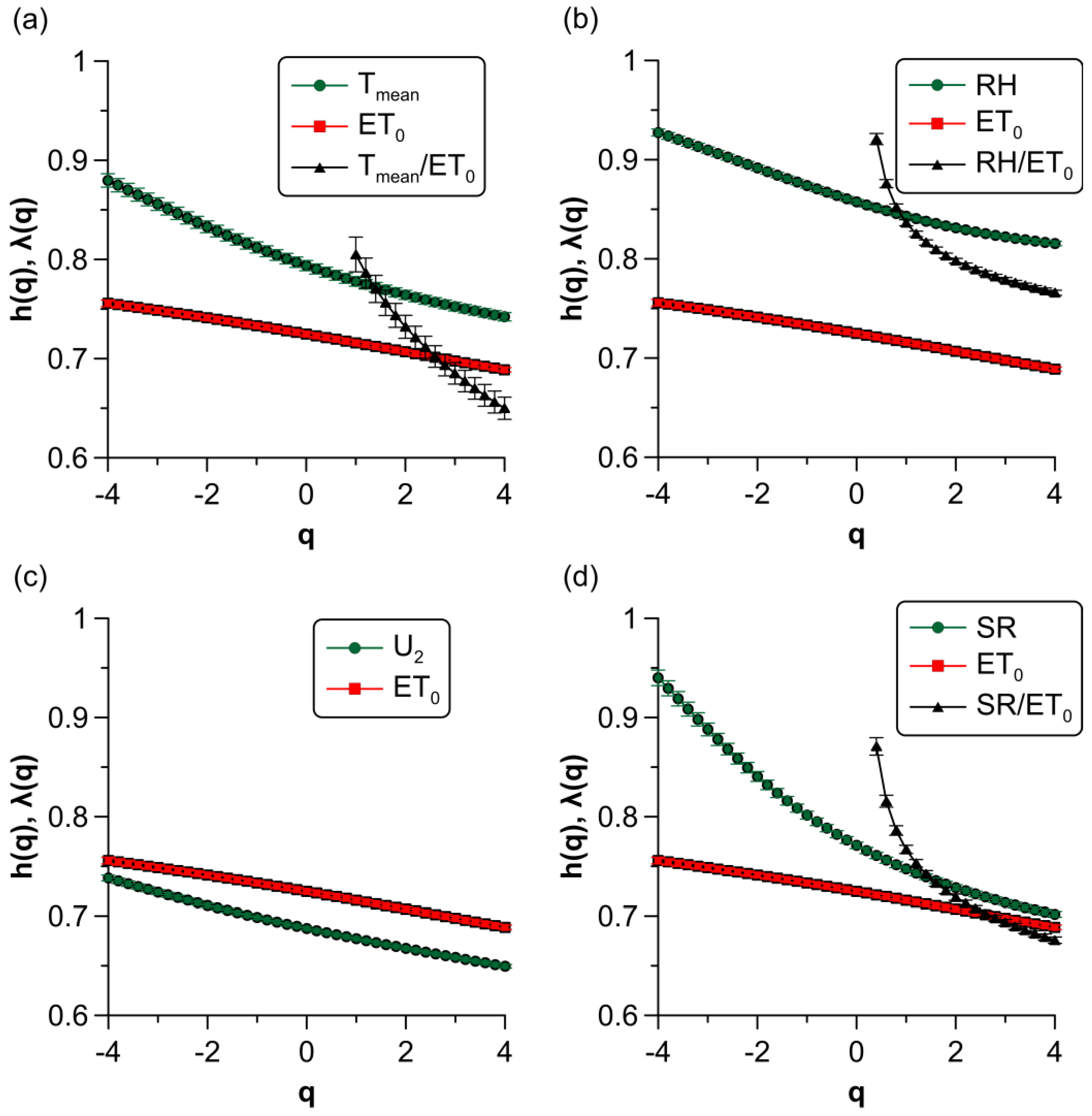
The multifractal cross-correlation exponents for in the –, –, and – links are shown in Figure 6 (black triangles) together with their individual scaling exponents (green and red symbols). They were obtained by fitting the covariance functions to a straight line in the ranges of scales , , and days, respectively (see Figure 5). can only be computed for in the case of the – relation and for in the other two cases. Pearson correlation coefficients from least-squares regressions were higher than 0.980 for every value of , and exponents were all higher than 0.5 and had larger statistical errors than their individual counterparts. Furthermore, they rapidly increased for medium fluctuations, showing a strong q-dependency and, thus, multifractal cross-correlations.
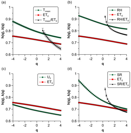
Figure 6.
Multifractal cross-correlation exponents, of meteorological variables with and their generalized Hurst exponents . (a) –. (b) . (c) . Multifractal cross-correlation was not observed in this case. (d) .
For the second-order moment, was approximately the average of the individual exponents, (see the small differences between both quantities, , in Table 3). However, for different values of , significantly deviated from for medium and relatively small fluctuations (Figure 6a,b,d) and for large fluctuations in the case of and (Figure 6a,d). This phenomenon has not been observed before in recent studies of the reference evapotranspiration, where multifractal correlation exponents stay within the range of the individual scaling exponents [17,19]. According to Oświȩcimka et al., the difference between and arises from distinct values of proportionality constants in the power law behavior of each process [25]. This fact suggests that the nature and dynamics of multifractality of the meteorological factors and differ considerably.

Table 3.
MFCCA parameters and Pearson correlation coefficient ( ) at a significance level of 0.01 of the agro-meteorogical series.
The multifractal spectra of relations which exhibited multifractal cross-correlations are depicted in Figure 7. These spectra were completely left-sided spectra () and their most relevant properties can be seen in Table 3. Spectral widths were lower than the width found for each individual variable, except for the – link (see Table 2 and Table 3), which might also be directly inferred from the wide range of exponents shown in Figure 6a. This means that infrequent higher singularities of were mainly governed by extreme temperature values, which is consistent with the conclusions drawn in a previous study [2].
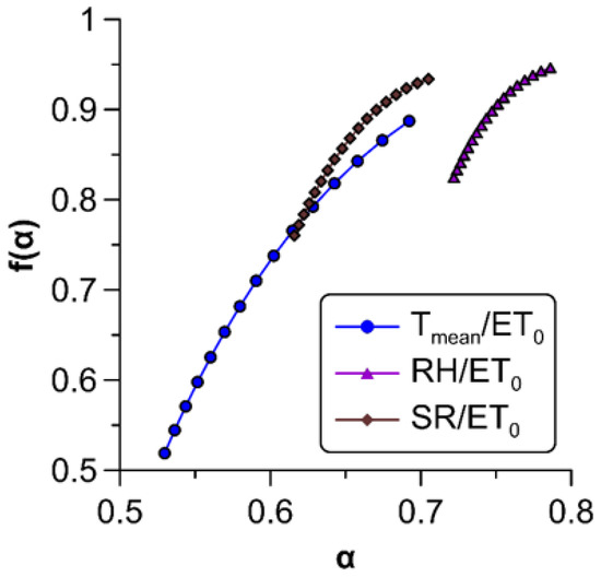
Figure 7.
Multifractal spectra of various pairs of cross-correlations with .
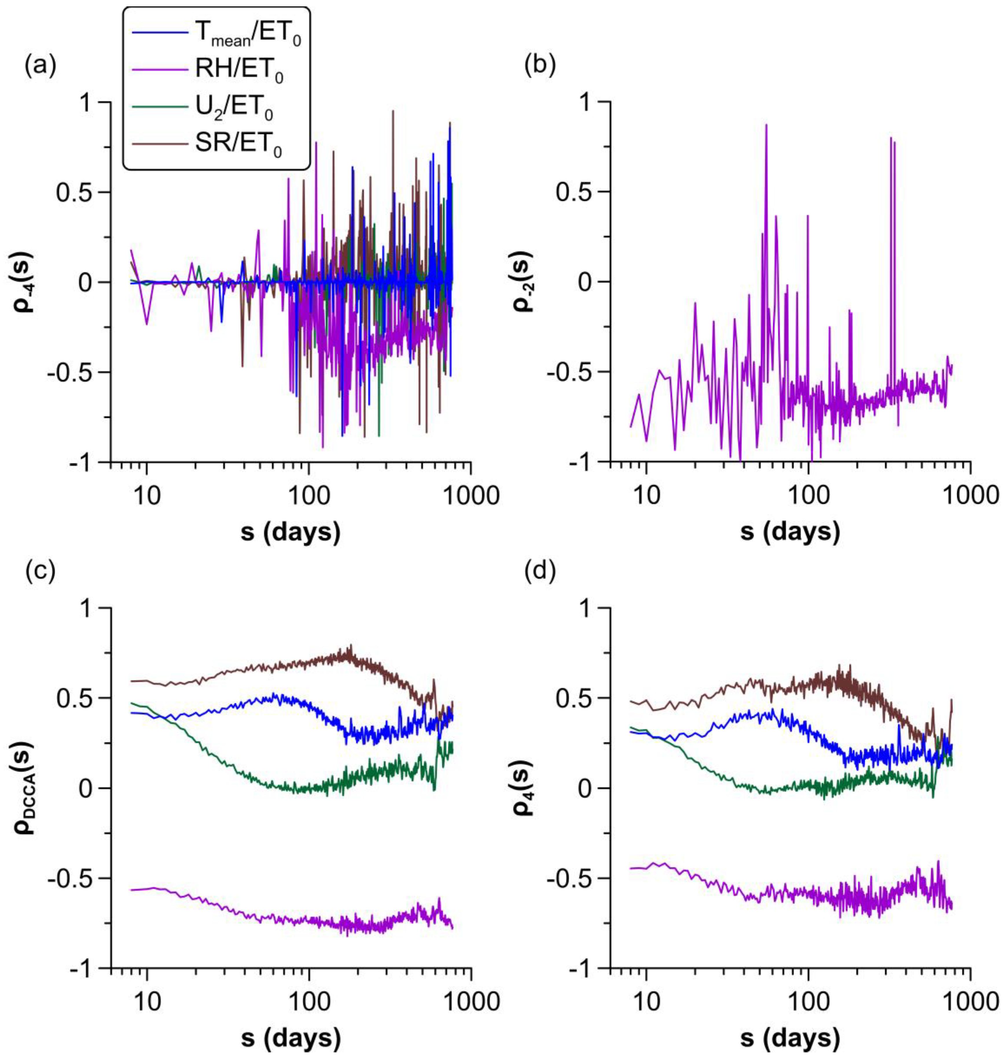
Lastly, Figure 8 shows the results of the q-dependent detrended cross-correlation coefficient, which allows us to quantify the strength of correlations between different pairs of links for fluctuations of different sizes.

Figure 8.
q-dependent detrended cross-correlation coefficients vs. the scale, , for different values of . (a) . (b) . Curves of the , – and links are omitted because of the presence of violent fluctuations in the range . (c) (). (d) .
Small and very small fluctuations of did not exhibit cross-correlations with any variable, since the normalized version of the coefficient fluctuated around zero or was highly unstable with violent fluctuations in the range (see Figure 8a,b and Section 2.3). For the sake of clarity, the coefficients for –, – and – links are not depicted in Figure 8b due to the extreme fluctuations observed in the range in these cases. Therefore, small fluctuations of (for ) do not show correlations with meteorological factors.
Medium-sized fluctuations, described by the standard DCCA coefficient , were weakly cross-correlated with all the analyzed meteorological factors for a wide range of scales, with the and being the most correlated ones. As was expected, the correlation between and was negative. Correlations were more stable and increased slightly with scale up to 60, 300, and 200 days (several months) for , , and , respectively. On the contrary, correlations slightly decreased with scale up to 50 days for , becoming negligible (see Figure 8c). For the first three variables, these bounds are closely related to the upper limits of the best scales where covariance functions fit well to power laws. From these boundaries, trends become more irregular and are inverted for large scales, except for , whose trend changes twice.
The Pearson correlation coefficients shown in Table 3 are close to the values of in every case, as occurred in a previous study [19]. Both coefficients clearly show the existence of some correlations which cannot be fitted to power-law behavior between and . Nevertheless, they are only significant for low timescales, from days to weeks, and are negligible for larger scales.
Very extreme events of can be analyzed for and these are correlated with all the meteorological factors, similarly to medium fluctuations, with a slight decrease in the strength of correlations in every case.
4. Conclusions
The behavior of five agro-meteorological variables in the middle zone of the Guadalquivir River Valley (south Spain) revealed time series with persistent long-range autocorrelations and multifractality. The variables , , and showed moderate persistence, while and exhibited the highest persistence, denoting more predictable signals. Furthermore, more precise results of multifractal properties than in a previous study [2] were obtained for , , and due to the elimination of trends in the original signals. The main controlling factors of , especially , displayed complex small fluctuations, whereas had more regular and homogeneous small fluctuations.
, , and exhibited multifractal cross-correlations with only for medium and large fluctuations. This suggests that complexity of is mainly due to relations between large events relating to various meteorological factors. On the contrary, previous studies performed in other regions have found multifractal cross-correlations for fluctuations of any magnitude [17,19]. Results of q-dependent cross-correlation exponents confirmed the absence of correlations for small fluctuations, whereas correlations existed for every variable for medium and large fluctuations. – and – links had the strongest correlations. Correlations between and were significant only for small scales, which indicates that does not influence the complexity of in the area analyzed.
Joint scaling exponents, , were close to the average of the individual scaling exponents for , whereas they differed for small and large fluctuations, meaning that some differences exist in the dynamics of multifractality among the analyzed variables. On the other hand, the singularity spectra showed that the – link had a wider spectra and higher singularities, which means that infrequent extreme events in are mainly ruled by high fluctuations of temperature, which is consistent with the results obtained in the previously mentioned study [2].
These conclusions allow confirmation of the usefulness of the MFCCA method in identifying multifractal cross-correlations when more than three variables are involved. Moreover, it has the advantage of being more easily interpretable than distributions of many dimensions obtained by the joint multifractal method.
Author Contributions
Conceptualization, J.G.-G. and A.B.A.-V.; methodology, J.G.-G.; software, J.G.-G.; validation, J.G.-G.; formal analysis, J.G.-G.; investigation, J.G.-G.; resources, J.G.-G. and A.B.A.-V.; data curation, J.G.-G.; writing—original draft preparation, J.G.-G.; writing—review & editing, J.G.-G.; visualization, J.G.-G.; supervision, A.B.A.-V., E.G.d.R., and F.J.J.-H.; project administration, E.G.d.R. and F.J.J.-H.; funding acquisition, E.G.d.R. and F.J.J.-H. The FLAE approach for the sequence of authors is applied in this work. All authors have read and agreed to the published version of the manuscript.
Funding
This research was funded by the European Regional Development Fund (Research project UCO-1379178, Operational Program Framework Andalusia 2014–2020) and the Andalusian Research Plan Group TEP-957.
Data Availability Statement
Publicly available datasets were analyzed in this study. This data can be found here: https://www.juntadeandalucia.es/agriculturaypesca/ifapa/riaweb/web/datosabiertos (accessed on 27 December 2022).
Acknowledgments
The authors gratefully acknowledge the support of the funding sources.
Conflicts of Interest
The authors declare no conflict of interest. The funding sponsors had no role in the design of the study; in the collection, analyses, or interpretation of data; in the writing of the manuscript; or in the decision to publish the results.
References
- Tabari, H.; Hosseinzadeh Talaee, P. Sensitivity of Evapotranspiration to Climatic Change in Different Climates. Glob. Planet. Change 2014, 115, 16–23. [Google Scholar] [CrossRef]
- Ariza-Villaverde, A.B.; Pavón-Domínguez, P.; Carmona-Cabezas, R.; Gutiérrez de Ravé, E.; Jiménez-Hornero, F.J. Joint Multifractal Analysis of Air Temperature, Relative Humidity and Reference Evapotranspiration in the Middle Zone of the Guadalquivir River Valley. Agric. For. Meteorol. 2019, 278, 107657. [Google Scholar] [CrossRef]
- Allen, R.G.; Pereira, L.S.; Raes, D.; Smith, M. Crop Evapotranspiration—Guidelines for Computing Crop Water Requirements—FAO Irrigation and Drainage Paper 56. Fao Rome 1998, 300, D05109. [Google Scholar]
- Doorenbos, J.; Pruitt, W.O. Guidelines for Predicting Crop Water Requirements. Irrig. Drain. Pap. (FAO) 1975, 24, 1–179. [Google Scholar]
- Gong, L.; Xu, C.; Chen, D.; Halldin, S.; Chen, Y.D. Sensitivity of the Penman–Monteith Reference Evapotranspiration to Key Climatic Variables in the Changjiang (Yangtze River) Basin. J. Hydrol. 2006, 329, 620–629. [Google Scholar] [CrossRef]
- Li, Y.; Qin, Y.; Rong, P. Evolution of Potential Evapotranspiration and Its Sensitivity to Climate Change Based on the Thornthwaite, Hargreaves, and Penman–Monteith Equation in Environmental Sensitive Areas of China. Atmos. Res. 2022, 273, 106178. [Google Scholar] [CrossRef]
- Jensen, M.E.; Burman, R.D.; Allen, R.G. Evapotranspiration and Irrigation Water Requirements. ASCE Manuals and Reports on Engineering Practices (USA) No. 70; American Society of Civil Engineers: New York, NY, USA, 1990; p. 332. [Google Scholar]
- López-Urrea, R.; Olalla, F.M.d.S.; Fabeiro, C.; Moratalla, A. An Evaluation of Two Hourly Reference Evapotranspiration Equations for Semiarid Conditions. Agric. Water Manag. 2006, 86, 277–282. [Google Scholar] [CrossRef]
- Nam, W.-H.; Hong, E.-M.; Choi, J.-Y. Has Climate Change Already Affected the Spatial Distribution and Temporal Trends of Reference Evapotranspiration in South Korea? Agric. Water Manag. 2015, 150, 129–138. [Google Scholar] [CrossRef]
- Sun, J.; Wang, G.; Sun, X.; Hu, Z.; Lin, S.; Wang, F.; Yang, Y. New Cognition on the Response of Reference Evapotranspiration to Climate Change in China Using an Independent Climatic Driver System. Agric. Water Manag. 2022, 262, 107445. [Google Scholar] [CrossRef]
- Yassen, A.N.; Nam, W.-H.; Hong, E.-M. Impact of Climate Change on Reference Evapotranspiration in Egypt. CATENA 2020, 194, 104711. [Google Scholar] [CrossRef]
- Oteros, J.; García-Mozo, H.; Vázquez, L.; Mestre, A.; Domínguez-Vilches, E.; Galán, C. Modelling Olive Phenological Response to Weather and Topography. Agric. Ecosyst. Environ. 2013, 179, 62–68. [Google Scholar] [CrossRef]
- Zhan, C.; Liang, C.; Zhao, L.; Zhang, Y.; Cheng, L.; Jiang, S.; Xing, L. Multifractal Characteristics Analysis of Daily Reference Evapotranspiration in Different Climate Zones of China. Phys. A Stat. Mech. Its Appl. 2021, 583, 126273. [Google Scholar] [CrossRef]
- Feder, J. Fractals; Springer US: Boston, MA, USA, 1988; ISBN 978-1-4899-2126-0. [Google Scholar]
- Mandelbrot, B.B. The Fractal Geometry of Nature; W.H. Freeman: San Francisco, CA, USA, 1982; ISBN 978-0-7167-1186-5. [Google Scholar]
- Gómez-Gómez, J.; Carmona-Cabezas, R.; Sánchez-López, E.; Gutiérrez de Ravé, E.; Jiménez-Hornero, F.J. Multifractal Fluctuations of the Precipitation in Spain (1960–2019). Chaos Solitons Fractals 2022, 157, 111909. [Google Scholar] [CrossRef]
- Adarsh, S.; Nityanjaly, L.J.; Pham, Q.B.; Sarang, R.; Ali, M.; Nandhineekrishna, P. Multifractal Characterization and Cross Correlations of Reference Evapotranspiration Time Series of India. Eur. Phys. J. Spec. Top. 2021, 230, 3845–3859. [Google Scholar] [CrossRef]
- Adarsh, S.; Sanah, S.; Murshida, K.K.; Nooramol, P. Scale Dependent Prediction of Reference Evapotranspiration Based on Multi-Variate Empirical Mode Decomposition. Ain Shams Eng. J. 2018, 9, 1839–1848. [Google Scholar] [CrossRef]
- Sankaran, A.; Krzyszczak, J.; Baranowski, P.; Devarajan Sindhu, A.; Kumar, N.; Lija Jayaprakash, N.; Thankamani, V.; Ali, M. Multifractal Cross Correlation Analysis of Agro-Meteorological Datasets (Including Reference Evapotranspiration) of California, United States. Atmosphere 2020, 11, 1116. [Google Scholar] [CrossRef]
- Sreedevi, V.; Adarsh, S.; Nourani, V. Multiscale Coherence Analysis of Reference Evapotranspiration of North-Western Iran Using Wavelet Transform. J. Water Clim. Change 2022, 13, 505–521. [Google Scholar] [CrossRef]
- Kantelhardt, J.W.; Zschiegner, S.A.; Koscielny-Bunde, E.; Havlin, S.; Bunde, A.; Stanley, H.E. Multifractal Detrended Fluctuation Analysis of Nonstationary Time Series. Phys. A 2002, 316, 87–114. [Google Scholar] [CrossRef]
- Plocoste, T.; Pavón-Domínguez, P. Multifractal Detrended Cross-Correlation Analysis of Wind Speed and Solar Radiation. Chaos 2020, 30, 113109. [Google Scholar] [CrossRef]
- Wątorek, M.; Drożdż, S.; Oświȩcimka, P.; Stanuszek, M. Multifractal Cross-Correlations between the World Oil and Other Financial Markets in 2012–2017. Energy Econ. 2019, 81, 874–885. [Google Scholar] [CrossRef]
- Zhang, C.; Ni, Z.; Ni, L. Multifractal Detrended Cross-Correlation Analysis between PM2.5 and Meteorological Factors. Phys. A Stat. Mech. Its Appl. 2015, 438, 114–123. [Google Scholar] [CrossRef]
- Oświȩcimka, P.; Drożdż, S.; Forczek, M.; Jadach, S.; Kwapień, J. Detrended Cross-Correlation Analysis Consistently Extended to Multifractality. Phys. Rev. E 2014, 89, 023305. [Google Scholar] [CrossRef]
- Podobnik, B.; Stanley, H.E. Detrended Cross-Correlation Analysis: A New Method for Analyzing Two Nonstationary Time Series. Phys. Rev. Lett. 2008, 100, 084102. [Google Scholar] [CrossRef] [PubMed]
- Kwapień, J.; Oświęcimka, P.; Drożdż, S. Detrended Fluctuation Analysis Made Flexible to Detect Range of Cross-Correlated Fluctuations. Phys. Rev. E 2015, 92, 052815. [Google Scholar] [CrossRef] [PubMed]
- Jiménez-Hornero, F.J.; Jiménez-Hornero, J.E.; Gutiérrez de Ravé, E.; Pavón-Domínguez, P. Exploring the Relationship between Nitrogen Dioxide and Ground-Level Ozone by Applying the Joint Multifractal Analysis. Environ. Monit. Assess. 2010, 167, 675–684. [Google Scholar] [CrossRef] [PubMed]
- Plocoste, T.; Pavón-Domínguez, P. Temporal Scaling Study of Particulate Matter (PM10) and Solar Radiation Influences on Air Temperature in the Caribbean Basin Using a 3D Joint Multifractal Analysis. Atmos. Environ. 2020, 222, 117115. [Google Scholar] [CrossRef]
- Zeleke, T.B.; Si, B.C. Characterizing Scale-Dependent Spatial Relationships between Soil Properties Using Multifractal Techniques. Geoderma 2006, 134, 440–452. [Google Scholar] [CrossRef]
- Gavilán, P.; Lorite, I.J.; Tornero, S.; Berengena, J. Regional Calibration of Hargreaves Equation for Estimating Reference ET in a Semiarid Environment. Agric. Water Manag. 2006, 81, 257–281. [Google Scholar] [CrossRef]
- García-Marín, A.P.; Jiménez-Hornero, F.J.; Ayuso-Muñoz, J.L. Multifractal Analysis as a Tool for Validating a Rainfall Model. Hydrol. Process. 2008, 22, 2672–2688. [Google Scholar] [CrossRef]
- Hu, K.; Ivanov, P.C.; Chen, Z.; Carpena, P.; Eugene Stanley, H. Effect of Trends on Detrended Fluctuation Analysis. Phys. Rev. E 2001, 64, 011114. [Google Scholar] [CrossRef]
- Kantelhardt, J.W.; Koscielny-Bunde, E.; Rybski, D.; Braun, P.; Bunde, A.; Havlin, S. Long-Term Persistence and Multifractality of Precipitation and River Runoff Records. J. Geophys. Res. 2006, 111, D01106. [Google Scholar] [CrossRef]
- Gong, H.; Fu, Z. Beyond Linear Correlation: Strong Nonlinear Structures in Diurnal Temperature Range Variability over Southern China. Chaos Solitons Fractals 2022, 164, 112737. [Google Scholar] [CrossRef]
- Rybski, D.; Bunde, A.; von Storch, H. Long-Term Memory in 1000-Year Simulated Temperature Records. J. Geophys. Res. 2008, 113, D02106. [Google Scholar] [CrossRef]
- Xavier Júnior, S.F.A.; Stosic, T.; Stosic, B.; Jale, J.D.S.; Xavier, É.F.M. A Brief Multifractal Analysis of Rainfall Dynamics in Piracicaba, São Paulo, Brazil. Acta Sci. Technol. 2018, 40, 35116. [Google Scholar] [CrossRef]
- Peng, C.-K.; Buldyrev, S.V.; Havlin, S.; Simons, M.; Stanley, H.E.; Goldberger, A.L. Mosaic Organization of DNA Nucleotides. Phys. Rev. E 1994, 49, 1685–1689. [Google Scholar] [CrossRef]
- Kantelhardt, J.W.; Rybski, D.; Zschiegner, S.A.; Braun, P.; Koscielny-Bunde, E.; Livina, V.; Havlin, S.; Bunde, A. Multifractality of River Runoff and Precipitation: Comparison of Fluctuation Analysis and Wavelet Methods. Phys. A 2003, 330, 240–245. [Google Scholar] [CrossRef]
- Zhang, Q.; Xu, C.-Y.; Chen, Y.D.; Yu, Z. Multifractal Detrended Fluctuation Analysis of Streamflow Series of the Yangtze River Basin, China. Hydrol. Process. 2008, 22, 4997–5003. [Google Scholar] [CrossRef]
- Baranowski, P.; Krzyszczak, J.; Slawinski, C.; Hoffmann, H.; Kozyra, J.; Nieróbca, A.; Siwek, K.; Gluza, A. Multifractal Analysis of Meteorological Time Series to Assess Climate Impacts. Clim. Res. 2015, 65, 39–52. [Google Scholar] [CrossRef]
- Gómez-Gómez, J.; Carmona-Cabezas, R.; Ariza-Villaverde, A.B.; Gutiérrez de Ravé, E.; Jiménez-Hornero, F.J. Multifractal Detrended Fluctuation Analysis of Temperature in Spain (1960–2019). Phys. A Stat. Mech. Its Appl. 2021, 578, 126118. [Google Scholar] [CrossRef]
- Kalamaras, N.; Tzanis, C.; Deligiorgi, D.; Philippopoulos, K.; Koutsogiannis, I. Distribution of Air Temperature Multifractal Characteristics Over Greece. Atmosphere 2019, 10, 45. [Google Scholar] [CrossRef]
- Sarker, A.; Mali, P. Detrended Multifractal Characterization of Indian Rainfall Records. Chaos Solitons Fractals 2021, 151, 111297. [Google Scholar] [CrossRef]
- Telesca, L.; Lovallo, M. Analysis of the Time Dynamics in Wind Records by Means of Multifractal Detrended Fluctuation Analysis and the Fisher–Shannon Information Plane. J. Stat. Mech. 2011, 2011, P07001. [Google Scholar] [CrossRef]
- Shimizu, Y.; Thurner, S.; Ehrenberger, K. Multifractal spectra as a measure of complexity in human posture. Fractals 2002, 10, 103–116. [Google Scholar] [CrossRef]
- Drożdż, S.; Minati, L.; Oświȩcimka, P.; Stanuszek, M.; Wątorek, M. Signatures of the Crypto-Currency Market Decoupling from the Forex. Future Internet 2019, 11, 154. [Google Scholar] [CrossRef]
- Vassoler, R.T.; Zebende, G.F. DCCA Cross-Correlation Coefficient Apply in Time Series of Air Temperature and Air Relative Humidity. Phys. A Stat. Mech. Its Appl. 2012, 391, 2438–2443. [Google Scholar] [CrossRef]
- Oświęcimka, P.; Drożdż, S.; Kwapień, J.; Górski, A.Z. Effect of Detrending on Multifractal Characteristics. Acta Phys. Pol. A 2013, 123, 597–603. [Google Scholar] [CrossRef]
- Makowiec, D.; Fuliński, A. Multifractal Detrended Fluctuation Analysis as the Estimator of Long-Range Dependence. Acta Phys. Pol. B 2010, 41, 1025–1050. [Google Scholar]
Disclaimer/Publisher’s Note: The statements, opinions and data contained in all publications are solely those of the individual author(s) and contributor(s) and not of MDPI and/or the editor(s). MDPI and/or the editor(s) disclaim responsibility for any injury to people or property resulting from any ideas, methods, instructions or products referred to in the content. |
© 2023 by the authors. Licensee MDPI, Basel, Switzerland. This article is an open access article distributed under the terms and conditions of the Creative Commons Attribution (CC BY) license (https://creativecommons.org/licenses/by/4.0/).

