Article

The Nonlinear Dynamics Characteristics and Snap-Through of an SD Oscillator with Nonlinear Fractional Damping

1
State Key Laboratory of Mechanical Behavior and System Safety of Traffic Engineering Structures, Shijiazhuang Tiedao University, Shijiazhuang 050043, China
2
Department of Engineering Mechanics, Shijiazhuang Tiedao University, Shijiazhuang 050043, China
*
Author to whom correspondence should be addressed.
Fractal Fract. 2022, 6(9), 493; https://doi.org/10.3390/fractalfract6090493
Submission received: 30 July 2022 / Revised: 17 August 2022 / Accepted: 18 August 2022 / Published: 2 September 2022
(This article belongs to the Special Issue Advances in Fractional Order Derivatives and Their Applications)

Abstract

:
A smooth and discontinuous (SD) oscillator is a typical multi-stable state system with strong nonlinear properties and has been widely used in many fields. The nonlinear dynamic characteristics of the system have not been thoroughly investigated because the nonlinear restoring force cannot be integrated. In this paper, the nonlinear restoring force is represented by a piecewise nonlinear function. The equivalent coefficients of fractional damping are obtained with an orthogonal function. The influence of fractional damping on the transition set, the amplitude–frequency response and the snap-through of the SD oscillator are analyzed. The conclusions are as follows: The nonlinear piecewise function accurately mimics the nonlinear restoring force and maintains a nonlinearity property. Fractional damping can significantly affect the stiffness and damping property simultaneously. The equivalent coefficients of the fractional damping are variable with regard to the fractional-order power of the excitation frequency. A hysteresis point, a bifurcation point, a frequency island, pitchfork bifurcations and transcritical bifurcations were discovered in the small-amplitude resonant region. In the non-resonant region, the increase in the fractional parameters leads to the probability of snap-through declining by increasing the symmetry of the attraction domain or reducing the number of stable states.

1. Introduction

Geometric nonlinearity is one of the three major nonlinear problems in engineering applications. Many engineering applications, such as vehicle suspension and gear driving systems, typically exhibit nonlinear characteristics. Nonlinear systems are made equivalent to linear systems to facilitate analytical calculations. In this process, the accurate nonlinear dynamics behavior of the nonlinear system cannot be obtained. If the system has been working at high intensity for a long time, the model errors caused by this equivalent linearization will accumulate. Therefore, establishing an accurate geometric nonlinear system model and analyzing the nonlinear dynamic behavior of the model can ensure the safe and stable operation of the system.
The smooth and discontinuous (SD) oscillator is a typical geometric nonlinear system. The system, which consists of one concentrated mass and two slanted springs, was simplified by a simply supported beam model [1]. The prototypical model of an SD oscillator is shown in Figure 1. This model has been widely used to study snap-through phenomena [2], energy-harvesting mechanisms [3], quasi-zero vibration isolators [4] and applications in many other fields.
In Figure 1, X ( t ) is the displacement of the oscillator, m is the mass, c is the damping coefficient, k is the stiffness of the springs, l is the constant distance and L is the original length of the spring. The dynamics model of the prototypical SD oscillator is:
m X ¨ ( t ) + c X ˙ ( t ) + 2 k X ( t ) 1 L X ( t ) 2 + l 2 = 0
This system (1) is made dimensionless by letting α = l / L ( α is the smooth parameter) ω 0 2 = 2 k / m , 2 ζ = c / m and x = X ( t ) / L :
x ¨ + 2 ζ x ˙ + ω 0 2 x 1 1 x 2 + α 2 = 0
where the nonlinear restoring force is F r e = ω 0 2 x 1 1 / x 2 + α 2 .
Notably, when the original length L is greater than the distance l ( 0 < α < 1 ), the oscillator has two stable positions (position 1 and position 3, as shown in Figure 1b). When the displacement or the velocity of the oscillator is smaller than the threshold, the oscillator vibrates at a small amplitude in stable position 1 or 3. If the displacement or the velocity of the oscillator exceeds the threshold (the threshold is the boundary of the attract domain, which will be discussed in Section 4), the oscillator will quickly jump from stable position 1 to stable position 3, or from 3 to 1. These stable position changes are called “snap-through”. However, when the original length L is smaller than the distance l ( α > 1 ), the oscillator has only one stable position (position 2). Thus, in this condition, the oscillator cannot change its stable position.
The dimensionless system parameters are selected as ω 0 2 = 2 , α = 0, 0.5, 1 and 1.5. Diagrams of the nonlinear restoring force F r e and the stiffness of the SD oscillator are shown in Figure 2.
Figure 2a shows the nonlinear restoring force with different smooth parameters, and Figure 2b shows the stiffness of the SD oscillator. In Figure 2a, the nonlinear restoring force has a jump point at x = 0 when α = 0 . In Figure 2b, the stiffness is negative in the neighborhood of x = 0 ( x 1 < x < x 2 ) when the smooth parameter is 0.5. The slope of F r e , i.e., the stiffness, approaches ω 0 2 when x approaches infinity. These phenomena indicate that the system is discontinuous when α = 0 , and it has a negative stiffness property when the smooth parameter is in the interval 0 < α < 1 . The system has a quasi-zero stiffness property when α = 1 . Additionally, its stiffness is positive when α > 1 .
SD oscillators have been widely used in many fields due to their special nonlinear properties. Researchers have conducted many in-depth studies on SD oscillators. Avramov et al. [5] connected an SD-like truss with a spring–mass system and investigated snap-through and nonlinear vibration characteristics. Brennan et al. [6] used an SD-like model with snap-through characteristics to represent the wings of dipteran insects. Their results show that the snap-through phenomenon resulted in a velocity jump in the system. When the operating frequency was below the natural frequency, the system had a great advantage in flight. Ichiro et al. [7] studied the nonlinear characteristics of an elastic–plastic system using a multi-folding microstructure system composed of SD structures. Waite et al. [8] investigated the attractor coexistence and the competing resonance of a truss with the SD structure. Hao et al. [9,10] designed a quasi-zero-stiffness vibration isolator based on an SD oscillator. Currier et al. [11] designed a mechanical fish that had an SD-like spine structure. The structure provided sufficient acceleration for the fish to swim. SD oscillators are also widely applied in nonlinear energy sinks [12,13] and energy harvesting [14,15]. Myongwon et al. [16] demonstrated a 1D lattice of bistable elements. The lattices exhibited energy-harvesting capabilities from transition waves, and energy was transmitted in the form of waves. Tan et al. [17] designed a triboelectric nanogenerator constituted by a bow-type Teng with a snap-through phenomenon. The equipment converted low-frequency vibrations into electricity with a high efficiency.
In terms of nonlinear dynamics, the trilinear piecewise function method [18] and the elliptic function method [19] have been proposed for investigating the nonlinear dynamics characteristics of SD oscillators. Subsequently, Tian et al. [20] studied the codimension-two bifurcation and the Hopf bifurcation of an SD oscillator. Cao et al. [21] analyzed the limit case response of an SD oscillator. In this case, the SD oscillator lost hyperbolicity due to a discontinuous characteristic that was different from a standard double-well system. Shen et al. [22] studied the bifurcation characteristics of symmetric subharmonic orbits and asymmetric subharmonic orbits of a discontinuous SD oscillator. Han et al. [23] used singularity theory to obtain the transition set of a coupled SD oscillator. The chaos threshold was obtained using the Melnikov method. [24] The multiple buckling and the codimension-three bifurcation of an SD oscillator were analyzed [25,26]. Tian et al. [27] studied the chaos threshold of an asymmetric SD oscillator subjected to constant excitation with the topological equivalence method. Yue et al. [28] investigated the random bifurcation of an SD oscillator based on the generalized cell-mapping method. In terms of the frequency domain, Santhosh et al. [29] found a chaotic solution for an SD oscillator caused by the symmetry breaking. Chen et al. [30,31] studied the global bifurcation characteristics of a discontinuous SD oscillator that was equivalent to a Filippov system. Wang et al. [32] represented fractional damping using a Markov chain. The random P bifurcation of an SD oscillator with fractional damping was studied. Their results show that both the smooth parameter and the excitation amplitude induced a random P-bifurcation of the SD oscillator. Through experiments, Chang et al. [33] proved that the periodic motion of an SD oscillator is highly sensitive to the initial displacement and the smooth parameter.
The nonlinear dynamic behaviors of SD oscillators with integral damping have been thoroughly studied. However, two limitations exist in the current research. One limitation is that the Taylor series expansion method is used to mimic the nonlinear restoring force in SD oscillators. The calculation accuracy of the equivalence transformation is acceptable when displacement responses are small. However, this can produce large errors if displacement responses are large. The other limitation is that the integer-damping model is used to represent the energy dissipation. However, in terms of long-term dynamic behaviors, the memory properties and frequency dependence characteristics are not well revealed. It is proven that these properties can be more accurately revealed by the fractional damping model [34,35]. Caputo et al. [36] proposed a fractional-order model to describe the dissipation characteristics, which correlate well with the experimental results of many materials. Padovan et al. [37] investigated the nonlinear response characteristics of a Duffing system with fractional damping. Chang et al. [38] proposed a nonlinear fractional damping model based on the Caputo fractional model [39]. The nonlinear fractional damping model described the energy-dissipation propertoes of metal rubber damping, and the theoretical solution fit well with the results of dynamic load experiments. Their results show that the fractional term simultaneously influenced the frequency and the amplitude of the response. However, research on the vibration characteristics of SD oscillators with fractional damping is not sufficient.
Combined with the current research status, it is necessary to study the nonlinear characteristics of SD oscillators with fractional damping. Therefore, in this article, an equivalent piecewise function is proposed for accurately representing the nonlinear restoring force of an SD oscillator. Moreover, a nonlinear fractional damping model is introduced into the SD oscillator to represent the energy dissipation and viscoelastic properties of a metal rubber damping. This article mainly focuses on the nonlinear amplitude–frequency response and transition characteristics in the resonant region and snap-through phenomena in the non-resonant region of the system. In Section 1, an introduction to this paper is presented. In Section 2, the nonlinear piecewise function is used to approximate the nonlinear restoring force of the SD oscillator. The equivalent damping coefficient and the equivalent stiffness coefficient of fractional damping are derived using the energy equivalent method. The piecewise differential equation of the SD oscillator with nonlinear fractional damping is obtained. In Section 3, the amplitude–frequency response function, the stable criteria and the transition set of the SD oscillator are obtained through calculations. In Section 4, the influence of fractional damping parameters on the nonlinear dynamic characteristics is analyzed in detail. The conclusions are provided in Section 5.

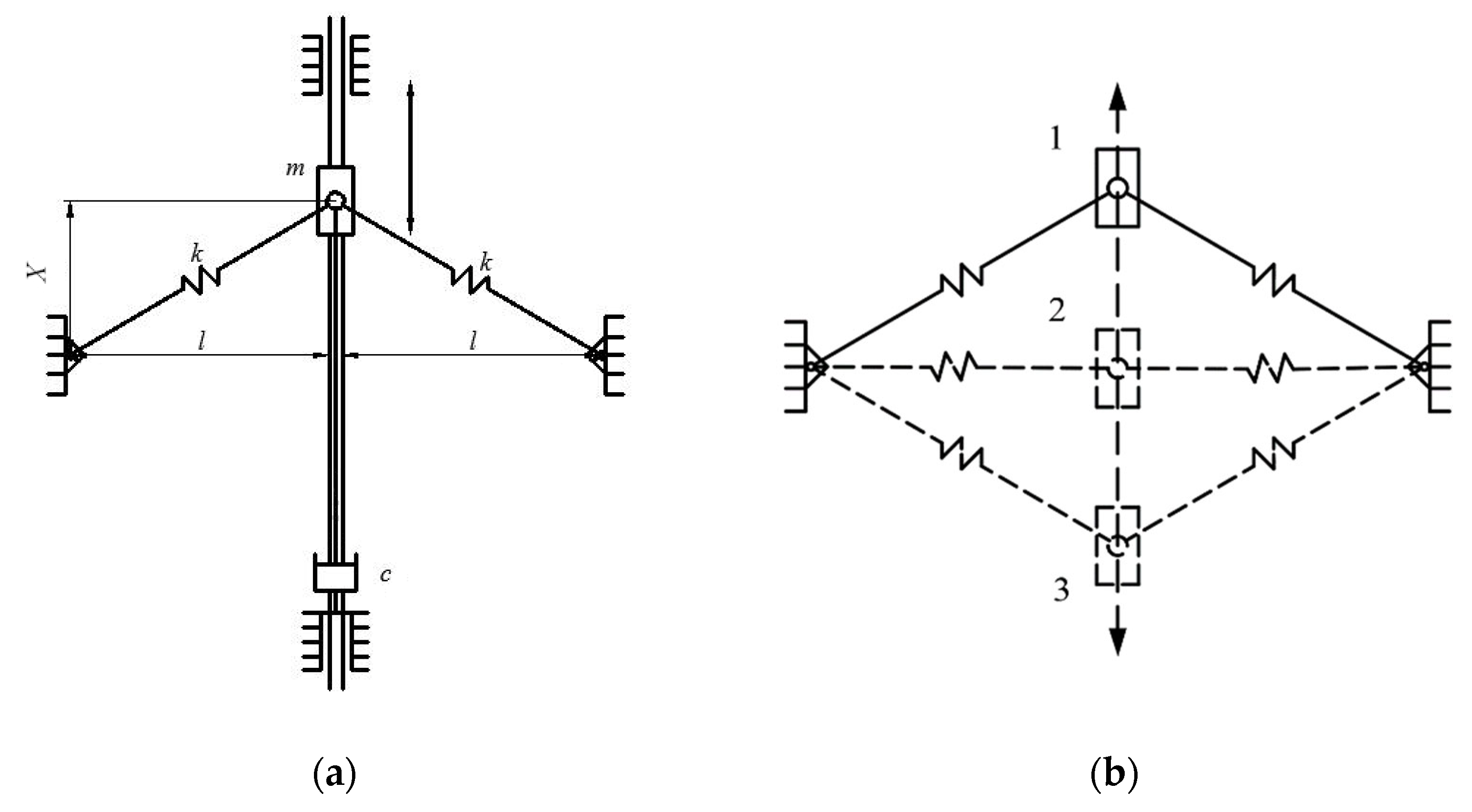
2. The Model of an SD Oscillator with Nonlinear Fractional Damping

The differential equation of the SD oscillator with nonlinear fractional damping is:
m X ¨ ( t ) + A ¯ ¨ + c X ˙ ( t ) + 2 k 0 X ( t ) 1 L X ( t ) 2 + l 2 + k 1 X ( t ) + k 3 X ( t ) 3 + h D p [ X ( t ) ] = 0
where A ¯ = A cos ω t is the external displacement excitation, A is the excitation amplitude, ω is the excitation frequency and X ( t ) is the displacement. F f r a c = k 1 X ( t ) + k 3 X ( t ) 3 + h D p [ X ( t ) ] is the damping force of a metal rubber damping [38], k 1 is the linear stiffness coefficient, k 3 is the nonlinear stiffness coefficient, h is the fractional coefficient, p is the fractional order and h D p [ X ( t ) ] is the Caputo fractional model [39,40]. The reason the Caputo model is selected is because its initial condition is the same form as the integer-order differential equation. It is convenient for addressing the problem of initial value in dynamics [41].
The new length scale L 1 and new time scale t 1 are selected as:
L 1 = L ,   t 1 = m k 1
The following dimensionless transformances are determined:
x ( τ ) = X ( t ) L ,   τ = t t 1 ,   2 ζ = c t 1 m ,   K 0 = 2 k 0 t 1 2 m ,   K 1 = k 1 t 1 2 m ,   K 3 = k 3 t 1 2 L 2 m ,   H = h t 1 2 m ,   α = l L ,   Ω = ω t 1 ,   F = A Ω 2 L
By substituting the above dimensionless transformances into Equation (3), we can rewrite the equation as:
x ¨ ( τ ) + 2 ζ x ˙ ( τ ) K 0 F n + K 1 x ( τ ) + K 3 x ( τ ) 3 + H D p [ x ( τ ) ] = F cos ( Ω τ )
The nonlinear restoring force of Equation (5) is defined as:
F n = x ( τ ) 1 1 x ( τ ) 2 + α 2
Equation (6) is nonintegral; therefore, the amplitude–frequency response function of the system cannot be obtained. The nonlinear piecewise function P n is introduced to obtain the equivalent function of Equation (6):
P n = x ( τ ) + B 1 , x ( τ ) < x 0 B 2 x ( τ ) 3 + B 3 x ( τ ) 2 + B 4 x ( τ ) , x 0 x ( τ ) < x 0 x ( τ ) + B 5 , x ( τ ) x 0
where B i i = 1 , 2 , 3 , 4 , 5 is undetermined constants and x 0 x 0 > 0 is the piecewise point of Equation (7).
F n is the first derivative with respect to τ . Let F n = 0 , and two extreme points ( x ˜ 1 , 2 , y ˜ 1 , 2 ) of Equation (6) can be obtained:
( x ˜ 1 , 2 , y ˜ 1 , 2 ) = ± α 4 / 3 α 2 , ± α 4 / 3 α 2 1 1 α 2 / 3
Let the middle segment of Equation (7) satisfy Equation (8), and we can obtain:
B 2 = α 4 / 3 α 2 / 3 2 1 + α 2 / 3 α 8 / 3 B 3 = 0 B 4 = 3 1 + α 2 / 3 2 α 2 / 3
Next, calculate the piecewise point x 0 and the corresponding function y 0 to obtain the constants B 1 and B 5 . Obviously, lim x F n = 1 , and the following can be set:
P n ( x 0 ) = 1
When x = x 0 , the piecewise point x 0 and the function y 0 of Equation (7) can be obtained:
x 0 = 1 3 1 α 2 / 3 α 4 / 3 + α 2 / 3 1 + α 2 / 3 α 8 / 3
y 0 = 1 3 α 2 / 3 4 α 2 / 3 + 3 α 2 / 3 3 3 α 10 / 3 α 4 / 3 + α 2 / 3 1 + α 2 / 3 α 8 / 3 3 / 2
Let the first and the third parts of Equation (7) satisfy the following conditions:
P n x 0 = y 0
P n x 0 = y 0
We can obtain B 1 and B 5 :
B 1 = 1 3 α 2 / 3 4 α 4 / 3 + α 2 / 3 3 + α 4 / 3 3 3 1 + α 2 / 3 α 10 / 3 α 4 / 3 + α 2 / 3 1 + α 2 / 3 α 8 / 3 3 / 2 B 5 = 1 3 α 2 / 3 4 α 4 / 3 α 2 / 3 3 + α 4 / 3 3 3 1 + α 2 / 3 α 10 / 3 α 4 / 3 + α 2 / 3 1 + α 2 / 3 α 8 / 3 3 / 2
By substituting Equations (9) and (15) into Equation (7), the nonlinear piecewise function is derived. By selecting α = 0.1, 0.5 and 0.9, the results of F n , P n , a linear piecewise function and a three-order Taylor series-equivalent function, are depicted in Figure 3.
Figure 3 shows that using the three-order Taylor series-equivalent function to approach F n is not effective because the deviation between curves for three-order Taylor series and F n sharply increases. The linear piecewise function and P n are in good agreement with F n . However, a larger error is generated at the extreme points of F n , and the nonlinear characteristics of the system are eliminated in the interval x 0 < x < x 0 , when the linear piecewise function is used to represent F n . By analyzing the curve of P n , it is found that P n correlates well with F n , and the nonlinear characteristics are maintained. Thus, many novel nonlinear phenomena have been discovered, such as the hysteresis point, the bifurcation point and transcritical bifurcation, which will be discussed in Section 4.
By substituting Equation (7) into Equation (5) to replace Equation (6), the differential equation of the SD oscillator with nonlinear fractional damping is written as:
x ¨ ( τ ) + 2 ζ x ˙ ( τ ) K 0 P n + K 1 x ( τ ) + K 3 x ( τ ) 3 + H D p [ x ( τ ) ] = F cos ( Ω τ )
The Caputo model [39] is used to represent the viscoelastic characteristics of nonlinear fractional damping, i.e., the fractional term in Equation (16):
D p [ X ] = 1 Γ ( 1 p ) 0 t X ( u ) t u p d u
where Γ ( ) is a gamma function.
When setting H D p [ x ( τ ) ] = c e q x ˙ ( τ ) + k e q x ( τ ) , sin ( φ ) and cos ( φ ) are multiplied on both sides. Both sides of the equations are integrated in one vibration period because the sum of the energy dissipated by damping and the energy stored by springs is a constant.
H Γ ( 1 p ) lim T 1 T 0 T 0 t a ω sin ( ω u + θ ) τ u p d u sin ( ω τ + θ ) d t = c e q a cos φ × sin φ d x H Γ ( 1 p ) lim T 1 T 0 T 0 t a ω sin ( ω u + θ ) τ u p d u cos ( ω τ + θ ) d t = k e q a cos φ × cos φ d x
where x ( τ ) = a cos Ω τ + θ = a cos φ .
Based on the orthogonality of trigonometric functions, the equivalent stiffness coefficient k e q and the equivalent damping coefficient c e q can be obtained as:
k e q = H Ω p cos p π 2 c e q = H Ω p 1 sin p π 2
It can be found that the fractional order p is the p th power or the ( p 1 ) th power of the excitation frequency Ω in Equation (19). Thus, c e q x ˙ ( τ ) + k e q x ( τ ) is a variable coefficient function with different values of power Ω because the response frequency in x ( τ ) and x ˙ ( τ ) is the same as the excitation frequency. Additionally, the fractional order p has different influences on k e q and c e q because of different values of the power. In terms of the vibration theory, fractional order p affects the stiffness property and the damping property of the system simultaneously.
Fractional order p is selected as 0, 0.3, 0.7 and 1. The results of the equivalent coefficients are depicted in Figure 4.
Figure 4a shows the results of the equivalent stiffness coefficient k e q . Figure 4b shows the results of the equivalent damping coefficient c e q . Figure 4 illustrates that k e q increases with increases in Ω , while c e q decreases. When Ω is above Ω 1 = e π tan ( p π / 2 ) / 2 , k e q first increases, then decreases as p increases (the variation tendency is marked by black arrows), while k e q monotonically decreases when Ω is smaller than Ω 1 = e π tan ( p π / 2 ) / 2 (the variation tendency is marked by red arrows). When Ω is above Ω 2 = e π cot ( p π / 2 ) / 2 , c e q monotonically increases as p increases (the variation tendency is marked by red arrows), while c e q first increases, then decreases when Ω is smaller than Ω 2 = e π cot ( p π / 2 ) / 2 (the variation tendency is marked by black arrows). When p equals 0, k e q and c e q equal H and 0, respectively. When p equals 1, k e q and c e q equal 0 and H , respectively. The above results illustrate that the fractional order and excitation frequency have a significant influence on the stiffness property and the damping property of the system simultaneously.
Substituting Equations (18) and (19) into Equation (16), the differential equation of the SD oscillator with a nonlinear fractional damping can be written as:
x ¨ ( τ ) + 2 ζ + H Ω p 1 sin p π 2 x ˙ ( τ ) K 0 P n + K 1 + H Ω p cos p π 2 x ( τ ) + K 3 x ( τ ) 3 = F cos Ω τ

3. The Bifurcation of the Amplitude–Frequency Response and the Stability Conditions of Steady-State Solutions

3.1. The Amplitude–Frequency Response Function of the Primary Resonance

The solution of Equation (20) is supposed as:
x ( τ ) = a cos Ω τ + θ = a cos φ
By substituting Equation (21) into Equation (20), and based on the average method, we can obtain:
a < x 0 :
a ˙ = 1 2 Ω 2 a ζ Ω + a H Ω p sin p π 2 + F sin θ a θ ˙ = 1 2 Ω a 4 3 a 2 B 2 K 0 + K 3 + 4 B 4 K 0 + K 1 Ω 2 + 4 H Ω p cos p π 2 F cos θ
a > x 0 :
a ˙ = 1 2 Ω 2 a ζ Ω + a H Ω p sin p π 2 + F sin θ a θ ˙ = 1 2 Ω K 0 π 2 B 1 + x 0 1 x 0 a 2 + K 0 π 2 B 5 + x 0 1 x 0 a 2 K 0 x 0 2 π 1 x 0 a 2 3 a 2 B 2 + 4 B 4 + 2 B 2 x 0 2 + 2 π a K 0 acos x 0 a + a 2 π K 0 asin ( x 0 a ) 3 a 2 B 2 + 4 B 4 + a K 1 + 3 4 a 3 K 3 a Ω 2 + a H Ω p cos p π 2 F cos θ
By eliminating θ , the amplitude–frequency response functions can be obtained as:
a < x 0 :
2 a ζ Ω + a H Ω p sin p π 2 2 + a 4 3 a 2 B 2 K 0 + K 3 + 4 B 4 K 0 + K 1 Ω 2 + 4 H Ω p cos p π 2 2 = F 2
a > x 0 :
2 a ζ Ω + a H Ω p sin p π 2 2 + K 0 π 2 B 1 + x 0 1 x 0 a 2 + K 0 π 2 B 5 + x 0 1 x 0 a 2 K 0 x 0 2 π 1 x 0 a 2 3 a 2 B 2 + 4 B 4 + 2 B 2 x 0 2 + 2 π a K 0 acos x 0 a + a 2 π K 0 asin x 0 a 3 a 2 B 2 + 4 B 4 + a K 1 + 3 4 a 3 K 3 2 a Ω 2 + a H Ω p cos p π 2 2 = F 2

3.2. The Stability Conditions of the Steady-State Solution

a = a ¯ + Δ a and θ = θ ¯ + Δ θ are substituted into Equations (22) and (23). a ¯ and θ ¯ are the singular points of Equations (22) and (23). Δ a and Δ θ are small disturbances. By eliminating θ ¯ , the following can be obtained:
a < x 0 :
d Δ a d t = R 11 Δ a R 12 Δ θ d Δ θ d t = R 13 Δ a R 14 Δ θ
a > x 0 :
d Δ a d t = R 11 Δ a R 21 Δ θ d Δ θ d t = R 22 Δ a R 14 Δ θ
The detail of R i , j i = 1 , 2 ; j = 1 , 2 , 3 , 4 is written in Appendix A.
Based on the Lyapunov theory, calculate the eigenvalues of the determinant, and the stability conditions of the steady-state solutions are:
a < x 0 :
R 11 + R 14 > 0 R 12 R 13 + R 11 R 14 > 0
a > x 0 :
R 11 + R 14 > 0 R 21 R 22 + R 11 R 14 > 0

3.3. The Transition Set of the Amplitude–Frequency Response Function

The unfolding functions are constructed by Equations (24) and (25).
a < x 0 :
G a , Ω , A , α = 2 a ζ Ω + a H Ω p sin p π 2 2 + a 4 3 a 2 B 2 K 0 + K 3 + 4 B 4 K 0 + K 1 Ω 2 + 4 H Ω p cos p π 2 2 F 2
a > x 0 :
G a , Ω , A , α = 2 a ζ Ω + a H Ω p sin p π 2 2 + K 0 π 2 B 1 + x 0 1 x 0 a 2 + K 0 π 2 B 5 + x 0 1 x 0 a 2 K 0 x 0 2 π 1 x 0 a 2 3 a 2 B 2 + 4 B 4 + 2 B 2 x 0 2 + 2 π a K 0 acos x 0 a + a 2 π K 0 asin x 0 a 3 a 2 B 2 + 4 B 4 + a K 1 + 3 4 a 3 K 3 a Ω 2 + a H Ω p cos p π 2 F cos θ 2 F 2
The excitation frequency Ω and the excitation amplitude A are defined as bifurcation parameters. Based on the singularity theory, the bifurcation plane of the amplitude–frequency response is derived. It is too complex to obtain the explicit formulation of the transition set. Therefore, the transition set obtained is
= B i f H y s
where B i f is the bifurcation set and H y s is the hysteresis set.
B i f = f , α 2 a , Ω , G = G a = G Ω = 0
H y s = f , α 2 a , Ω , G = G a = G a a = 0
The specific formulations of Equations (33) and (34) are written in Appendix B.

4. The Nonlinear Characteristics Analysis of the SD Oscillator with Nonlinear Fractional Damping

4.1. The Nonlinear Characteristics in the Resonant Region

First, the correctness of Equations (24) and (25) should be verified. The ODE45 method is used to calculate the numerical solutions to obtain the amplitude–frequency response of the system. The calculation step t s t e p = 0.0025 . Only forced vibration phenomena are concerned, so that the initial displacement and the initial velocity are zero to exclude the influence of transient resonance. Thus, the results of the numerical solution, Equations (24) and (25) are shown in Figure 5.
Figure 5 displays the results of the amplitude–frequency response of Equations (24) and (25), and the numerical solution. The pink dashed line represents the vibration amplitude a = x 0 . The blue and green solid lines represent the stable solutions calculated by Equations (24) and (25), respectively, while the unstable solution is drawn as a green dashed line. Circles are the numerical solution. The numerical solution is in good agreement with the theoretical solution. The correctness of Equations (24) and (25) is verified.

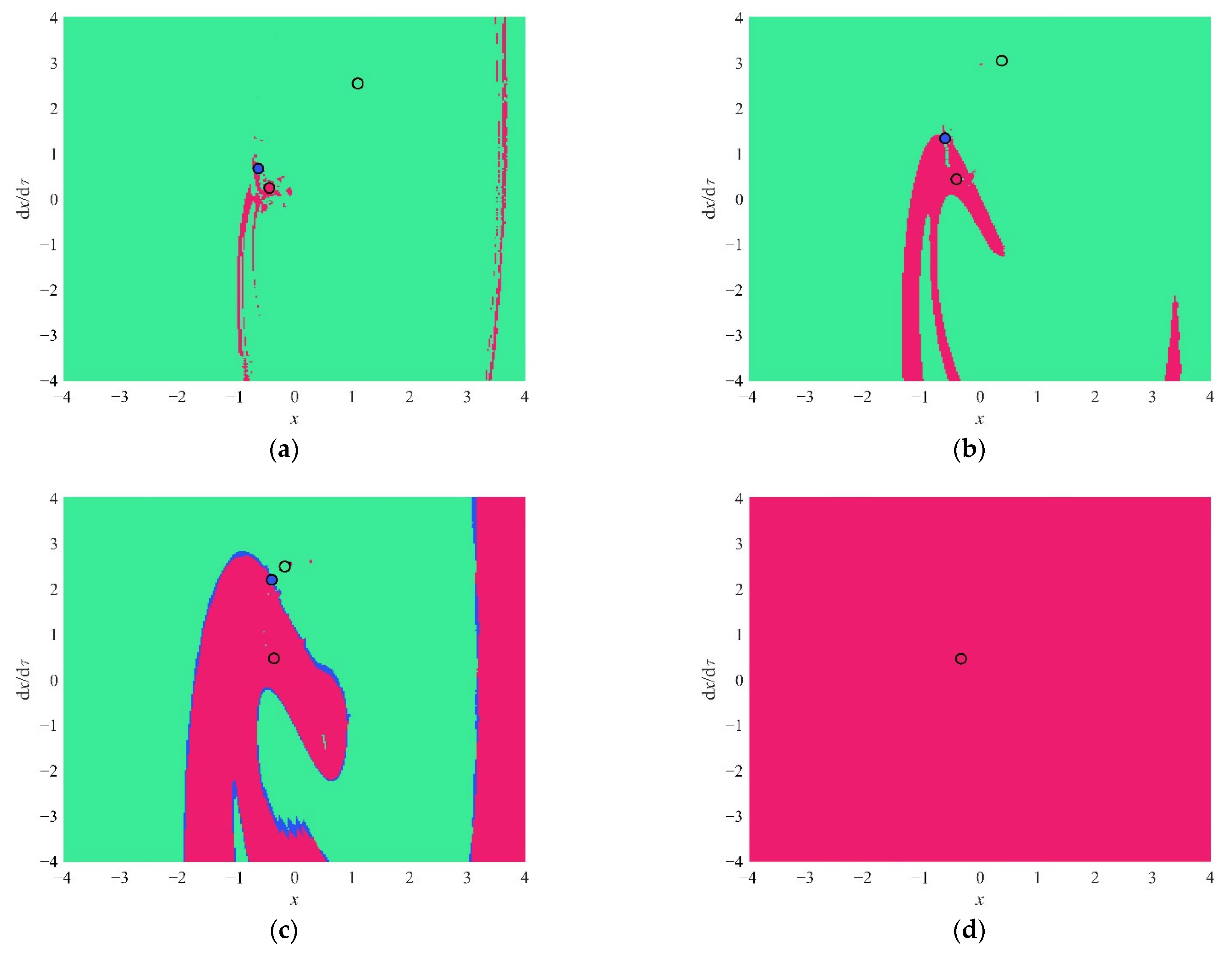
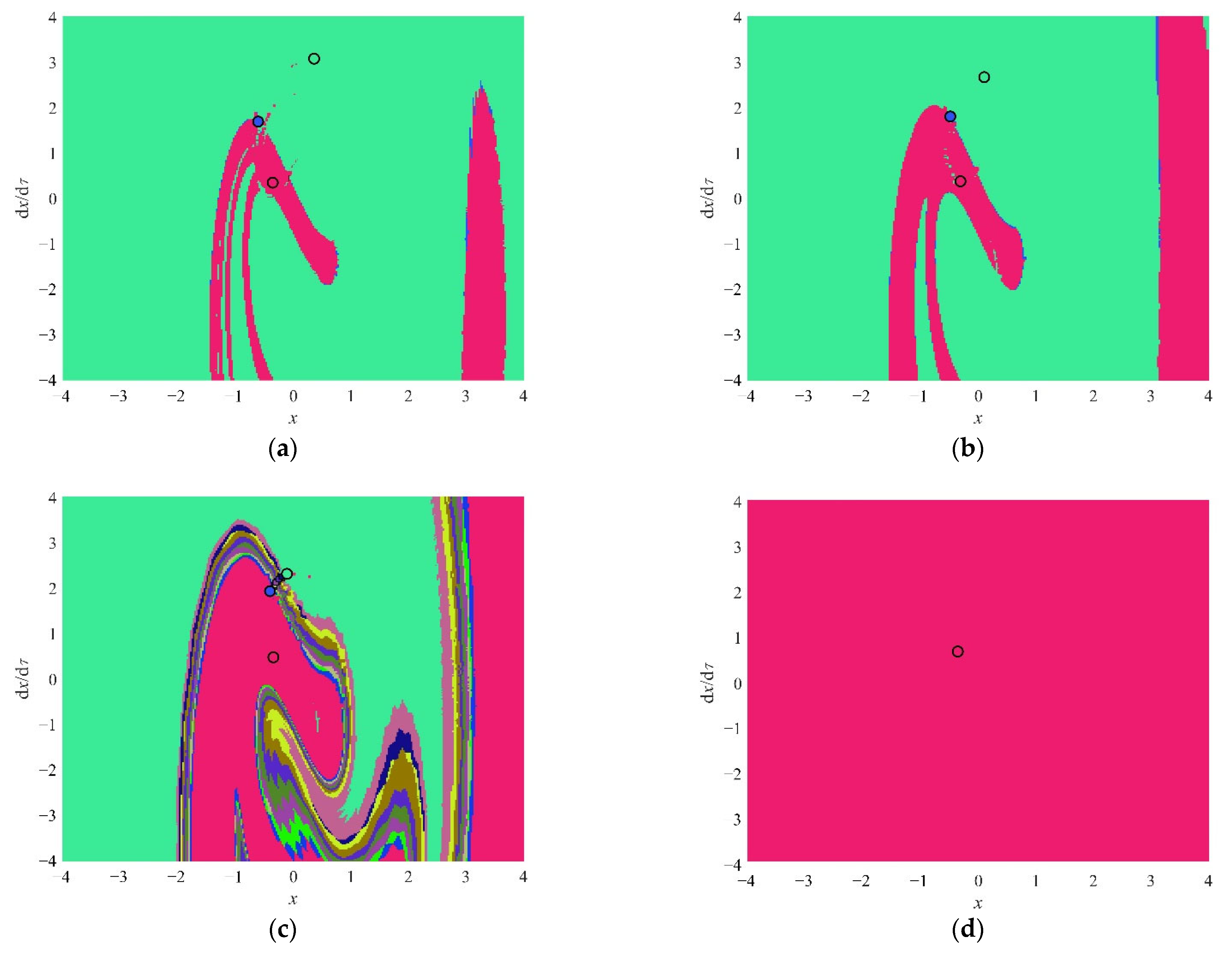
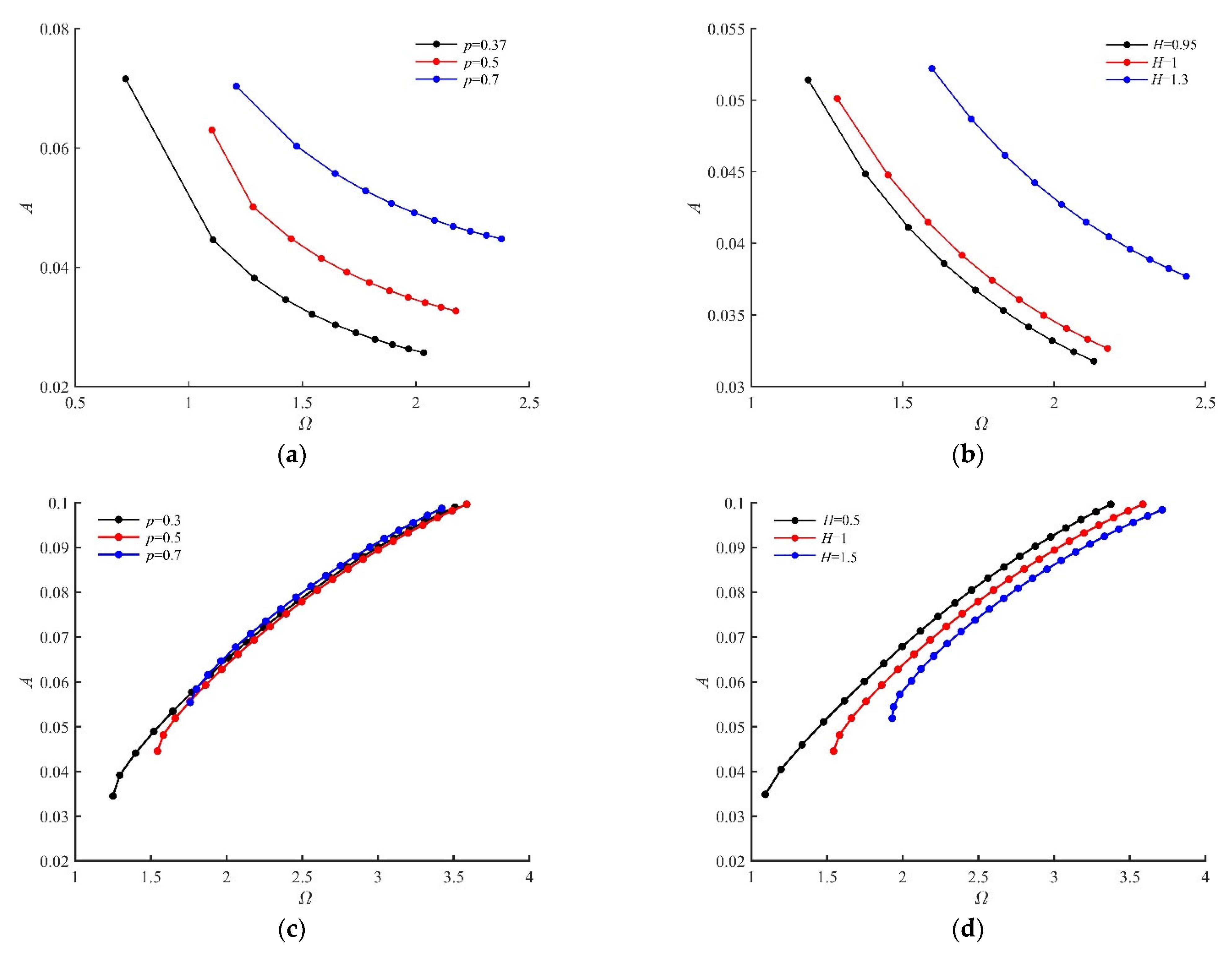
4.1.1. The Influence of the Smooth Parameter in the Transition Set of the System

Based on Equation (32), the influence of the smooth parameter and excitation parameters in the amplitude–frequency response is studied. The parameters selected are ζ = 0.1443 , K 0 = 20 , K 1 = 1 , K 3 = 0.0128 , H = 1 , and α [ 0.89 , 0.99 ] . The transition set, the amplitude–frequency response curves and the distribution of the attractors in the frequency island are depicted in Figure 6.
Figure 6a,b show the results of the bifurcation set and the hysteresis set of Equations (33) and (34), respectively. The explicit function of the bifurcation set and the hysteresis set cannot be directly obtained because the expressions of Equations (33) and (34) are too complex. Thus, in Figure 6a, three surfaces, G = 0 (the red surface), G a = 0 (the green surface) and G Ω = 0 (the blue surface), are drawn in the three-dimension space ( Ω , A , a ) , and their intersection B i f 1 = 1.6606 , 0.051901 , 0.38956 is obtained as the numerical solution of the bifurcation set. Using the same numerical method, in Figure 6b, the result of the hysteresis set H y s 1 = 1.0149 , 0.06301 , 0.34944 can be obtained, and the red surface is G = 0 , the green surface is G a = 0 , and the blue surface is G a a = 0 . After obtaining the transition set, all of the bifurcation conditions of the amplitude–frequency response of the SD oscillator can be calculated.
As shown in Figure 6c, a hysteresis point is generated, as the smooth parameter α equals 0.89. The hysteresis phenomenon leads to the appearance of pitchfork bifurcation. Comparing the green curve and the red curve in Figure 6c, the number of the results of a increases from 1 to 3 in the interval 0.5 < Ω < 1.5 , so that a new multi-solution coexistence region is generated. When α = 0.8594, a bifurcation point is generated. The bifurcation phenomenon leads to the appearance of transcritical bifurcation. Subsequently, a frequency island, which is depicted by closed black curves, occurs in the resonant region. There are three coexistent attractors in the entire region of the frequency island. The three attractors are depicted in Figure 6d by orange, purple and cyan circles, respectively. The attraction domains are drawn in the same colors as the attractors. The orange attractor is a stable attractor with the largest amplitude and the widest attraction domain, corresponding to the top black branch of the frequency island; the purple attractor is a stable attractor with the smallest amplitude and a narrow attraction domain corresponding to the bottom black solid line; and the other unstable attractor corresponds to the black dashed line in Figure 6c.
The above novel nonlinear phenomena in the small amplitude region are disclosed due to the fact that the nonlinear piecewise function P n maintains the nonlinear property of the system in the interval x 0 < x < x 0 . Because of the frequency island, the vibration amplitude of the SD oscillator can be adjusted by imposing a disturbance to change the displacement or the velocity in order to make them exceed the boundary of the attraction domain.
Next, the frequency island is further analyzed in terms of the distributions of the attractors and the time history of vibration. Thus, the distribution of attractors in the frequency island, the time history of vibration of stable attractors and those without the frequency island are drawn in Figure 7 and Figure 8. To highlight the differences, the parameters in Figure 7 and Figure 8 are selected as Ω = 2 , α = 0.85 and Ω = 2 , α = 0.9 , respectively.
Figure 7a shows that two stable attractors (the orange circle and the purple circle) with different amplitudes coexist with an unstable attractor (the cyan circle) in the frequency island. Figure 7b shows the time history of vibration. The stable motion in the black line corresponds to the orange attractor in Figure 7a, and the stable motion in the red line corresponds to the purple attractor in Figure 7a. In Figure 7a, the black arrows and black dots are schematic representations of the attractor-switching phenomenon, supposing a disturbance is imposed in the system, which is in the stable state of the orange attractor. The displacement and the velocity of the system are changed to the first black dot, which marks that the system has entered the purple attraction domain. After a period of time, the system goes through several unstable states (the other black dots) before finally returning to a stable state (the purple circle). The vibration characteristic also changes from the black line to the red line in Figure 7b, and the vibration amplitude significantly decreases. However, without the frequency island, this phenomenon cannot be generated because there is only one attractor, as shown in Figure 8.
In Figure 8a, there is only one stable attractor, and the attraction domain is full of the entire state space. Thus, no matter what the initial conditions are, for example 1 , 0 or 0 , 0 , the stable state of the system can always be represented by the red line in Figure 8b. For most nonlinear systems, a narrow hysteresis region where the attractor-switching phenomenon can be generated, such as 2.5 < Ω < 4.1 in Figure 6c, is found in the resonant region. It is rare that the frequency island results in the entire resonant region generating the attractor-switching phenomenon.

4.1.2. The Influence of the Fractional Damping Parameters in the Transition Set of the System

From the above investigations, when the smooth parameter α decreases and nonlinearity increases, a transition process is disclosed: a hysteresis point followed by a bifurcation point and a frequency island. Further, with the frequency island, the fractional SD oscillator has a novel attractor-switching phenomenon among the entire resonant region. Thus, it is worth investigating the influence of the fractional damping parameters on the transition set. The results of the transition sets with different fractional damping parameters are shown in Figure 9.
Figure 9a,b show the influence of the fractional damping parameters on the hysteresis set of the system. As the fractional parameters increase, the hysteresis point requires the generation of a larger excitation amplitude and higher excitation frequency. In other words, the hysteresis point moves to the high-frequency and large-amplitude region. Figure 9b,c exhibit the influence of the fractional damping parameters in the bifurcation set. As the fractional damping order p increases, the bifurcation point moves to the high-frequency region, but the excitation amplitude has little change. As the fractional damping coefficient H increases, the bifurcation point moves to the high-frequency and small-amplitude region. In other words, the system needs a small excitation amplitude to generate a bifurcation point.
After analyzing the influence of the fractional damping on the hysteresis set and the bifurcation set, the influence of these parameters in the frequency island is investigated. The smooth parameter is selected as α = 0.7 . The amplitude–frequency response curves with different fractional damping parameters are drawn in Figure 10.
Figure 10 shows the amplitude–frequency response curves with differential fractional damping parameters. With the increase in the fractional parameters, both the frequency interval and amplitude of the stable solution in the frequency island decrease. When p = 0.9 in Figure 10a and H = 3.5 in Figure 10b, the frequency island disappears, while the stable solution with a small amplitude remains. The amplitude of the existing attractor decreases as the fractional order increases, while the amplitude increases as the fractional coefficient increases. The results correlate well with Figure 4, because with the fractional order equals 1 and Ω > Ω 2 = e π cot ( p π / 2 ) / 2 , the fractional damping has the equivalent of linear damping and is the strongest damping effect, causing the amplitude to decrease. As the fractional coefficient increases and Ω > Ω 1 = e π tan ( p π / 2 ) / 2 , the fractional damping has a stiffness property and a damping property, but the stiffness property is dominated, causing the amplitude to slightly increase.
To further investigate the reason why the frequency island disappears, the distribution of attractors in the frequency island is depicted in Figure 11 and Figure 12.
In Figure 11 and Figure 12, the stable attractor with a large amplitude is drawn in green, the stable attractor with a small amplitude is drawn in red and the unstable attractor is drawn in dark blue. These figures show the influence of the fractional parameters on the attractors in the frequency island. Figure 11 shows that as the fractional order increases, the green attractor moves closer to the blue attractor; meanwhile, the red attraction domain expands. Then, the green attractor collides with the blue attractor and disappears, while the red attraction domain fills the entire state space since p = 0.7 . This is the reason why the frequency island disappears as the fractional order increases.
Figure 12 shows that as the fractional coefficient increases, the green attractor collides with the blue attractor and becomes a new chaotic attractor (the chaotic attraction domain and the chaotic attractor are multicolored in Figure 12c). Subsequently, the chaotic attractor disappears; meanwhile, the red attraction domain expands until it fills the entire state space as shown in Figure 12d. This is the reason why the frequency island disappears as the fractional coefficient increases.

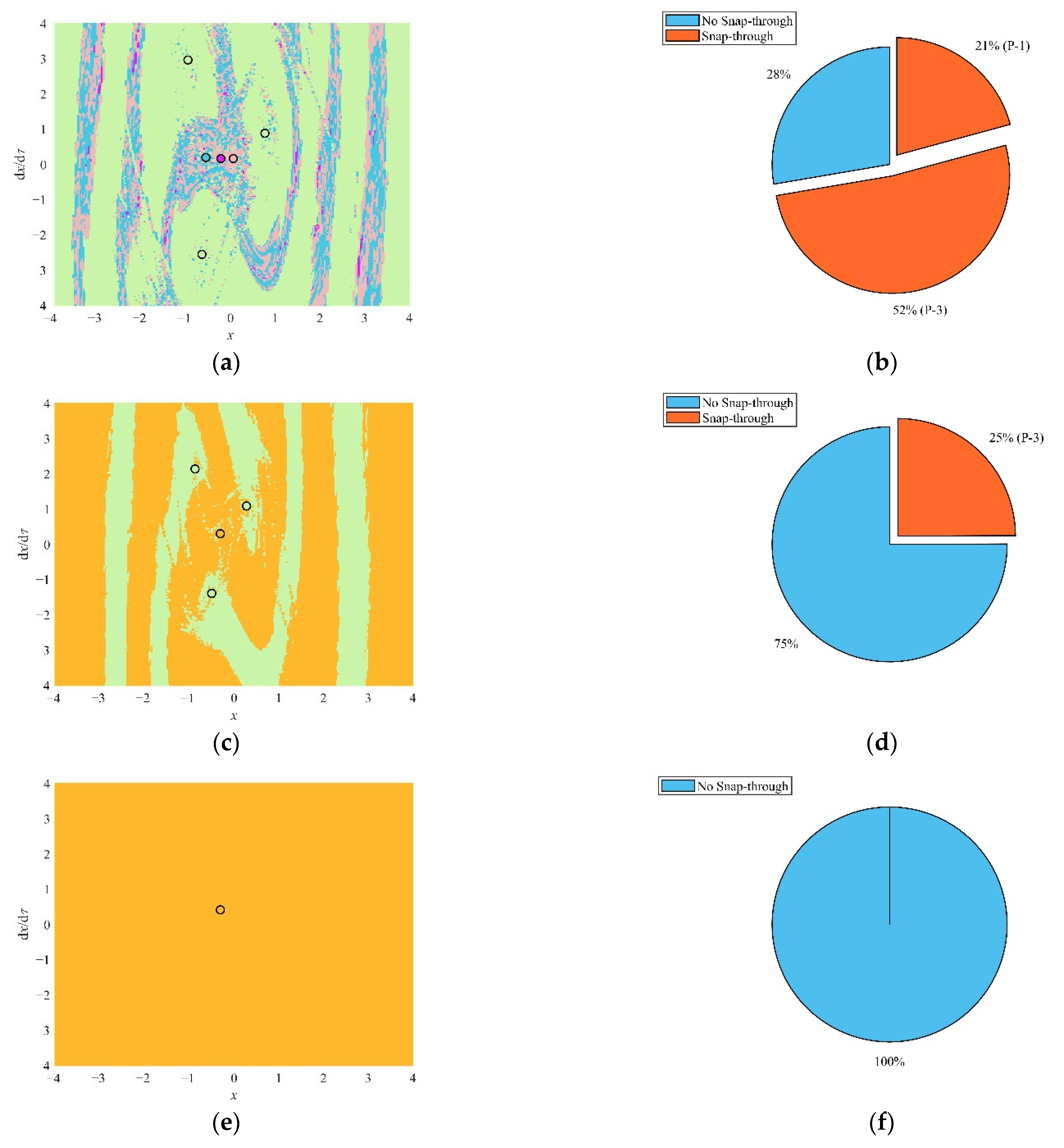
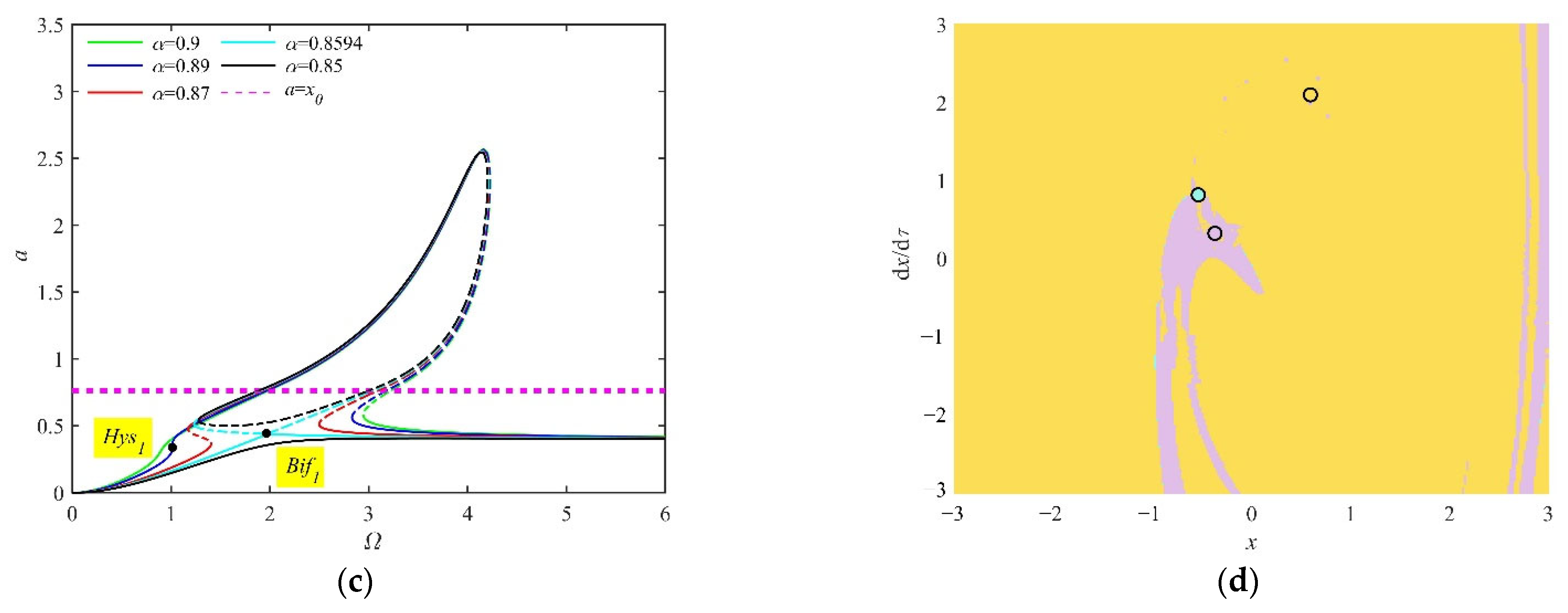
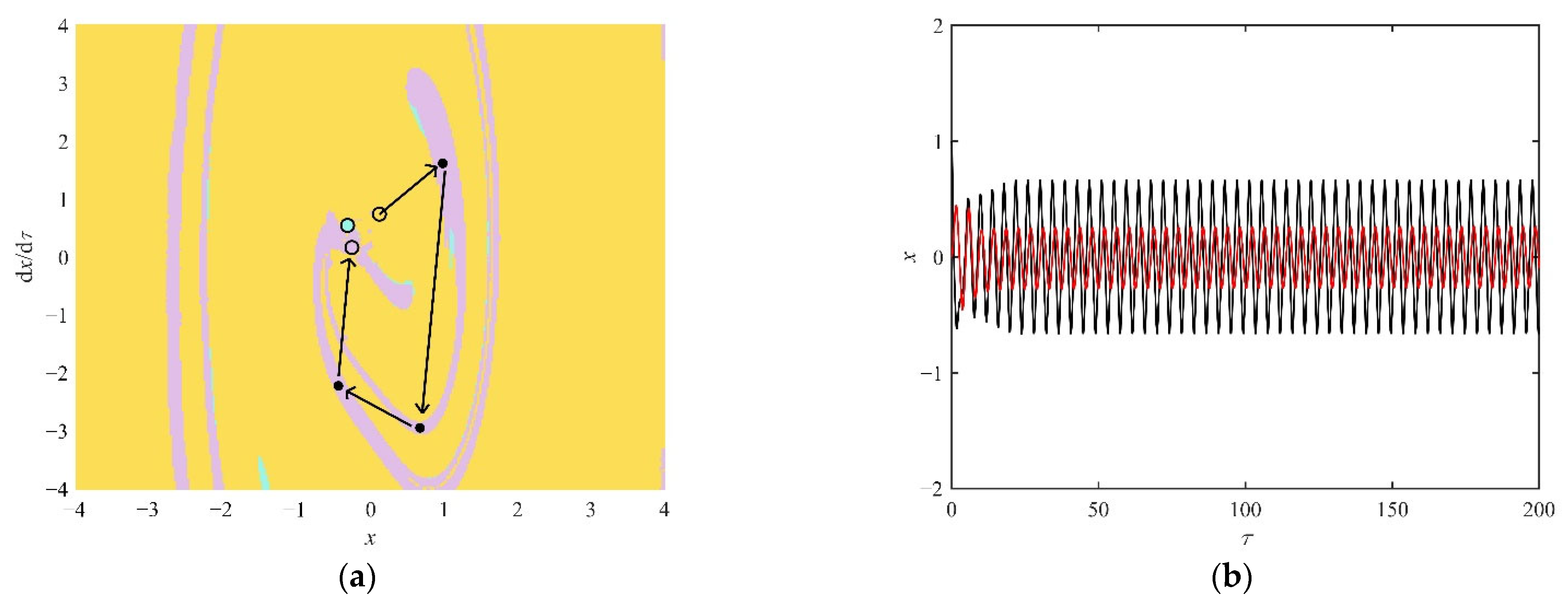
4.2. Analysis of the Snap-Through Phenomenon in the Non-Resonant Region

In the non-resonant region, this article mainly focuses on the snap-through phenomenon that is commonly discovered in multi-well dynamics systems. A multi-well system which generates snap-through phenomena has been analyzed in terms of the nonlinear energy and the competing resonance. When the energy is sufficient to exceed the energy threshold of the potential well, two types of transition phenomena are generated: one is inner-well motion → inter-well motion → inner-well motion (it is a different potential well from the initial well), and the other is inner-well motion → inter-well motion [8,12].
In this section, the influence of the fractional parameters on the snap-through phenomenon in the non-resonant region is analyzed in terms of the global dynamics. The distribution of attractors is obtained when Ω = 1 (the frequency is lower than the natural frequency) and 8.5 (the frequency is higher than the natural frequency). The initial displacement x s and the initial velocity x ˙ s are selected as x s , x ˙ s = 0.7 , 0 to keep the steady-state motion of the system corresponding to the same initial attractor. The random impulse disturbance, which has an amplitude of x i m 1 , 4 , is applied 100 times, and the experiment is repeated 100 times. The probabilities that the system generates snap-through due to the random disturbance and the distribution of attractors in the non-resonant region are shown in Figure 13, Figure 14, Figure 15 and Figure 16.
Figure 13a,b show that the distribution of the attraction domain is helicoid. Two stable attractors (the cyan circle and the pink circle) and one unstable attractor (the purple circle) coexist. By increasing the fractional order, the continuity of the attraction domain increases, and the symmetry enhances. Thus, as shown in Figure 13c,d, the probability of the snap-through decreases from 62% to 40%, which means that the asymptotic stability of the steady-state solution increases.
Figure 14a,b show that by increasing the fractional coefficient, the continuity of the attraction domain of the stable solutions increases, and the symmetry enhances. The probability of the snap-through decreases from 54% to 28% in Figure 14c,d. The asymptotic stability of the steady-state solution increases.
When the excitation frequency is smaller than the natural frequency, the increase in the fractional parameters leads to the continuity and symmetry of the attraction domain of the stable solution increasing. Meanwhile, the asymptotic stability of the steady-state solution increases.
Figure 15a shows that when the excitation frequency is larger than the natural frequency, one stable period-three attractor (the green circles) and three period-one attractors coexist. The attraction domain of the period-one attractors is discontinuous and narrow, which means that the asymptotic stability of the period-one motion is weak. The probability of the snap-through is 77%, which is shown in Figure 15c. By increasing the fractional order, the continuity of the period-one attraction domain increases, and the period-three attractor disappears (the existence conditions of the period-three are broken), as shown in Figure 15b. The probability of the snap-through decreases from 77% to 47%. Note that the two period-one attraction domains are still asymmetric; therefore, the probability of the snap-through in Figure 15d is higher than that in Figure 13d.
Figure 16a,c,e show that by increasing the fractional coefficient, three period-one attractors merge and evolve to a period-one attractor, and the period-one attraction domain expands. The asymptotic stability of the period-one motion increases. Meanwhile, the period-three attractor disappears because the existence condition of the period-three motion is broken. As the fractional coefficient equals 4, the period-three attractor disappears, while the period-one attraction domain fills the entire state space, as shown in Figure 16e. The system evolves from a tristable state to a bistable state and finally to a monostable state. Figure 16b,d,f illustrate that as the continuity of the attraction domain increases, the probability of the snap-through decreases from 73% to 0%. No snap-through occurs when the system is monostable, as shown in Figure 16f.
When the frequency is greater than the natural frequency, caused by an increase in the fractional coefficient, the asymptotic stability of the steady-state solution increases, and the number of the coexisting attractors changes. Thus, the probability of the snap-through decreases. This influence is different from the increase in the fractional order.

5. Conclusions

A new nonlinear piecewise function is proposed to establish the differential equation of the SD oscillator with fractional damping. The Caputo fractional model was used to represent the fractional damping, and the equivalent stiffness coefficient and the equivalent damping coefficient were calculated. The nonlinear dynamics characteristics and snap-through phenomena were studied. The influence of fractional damping on nonlinear dynamic characteristics was analyzed, and some novel and interesting nonlinear phenomena were disclosed. The conclusions from the investigation are as follows:
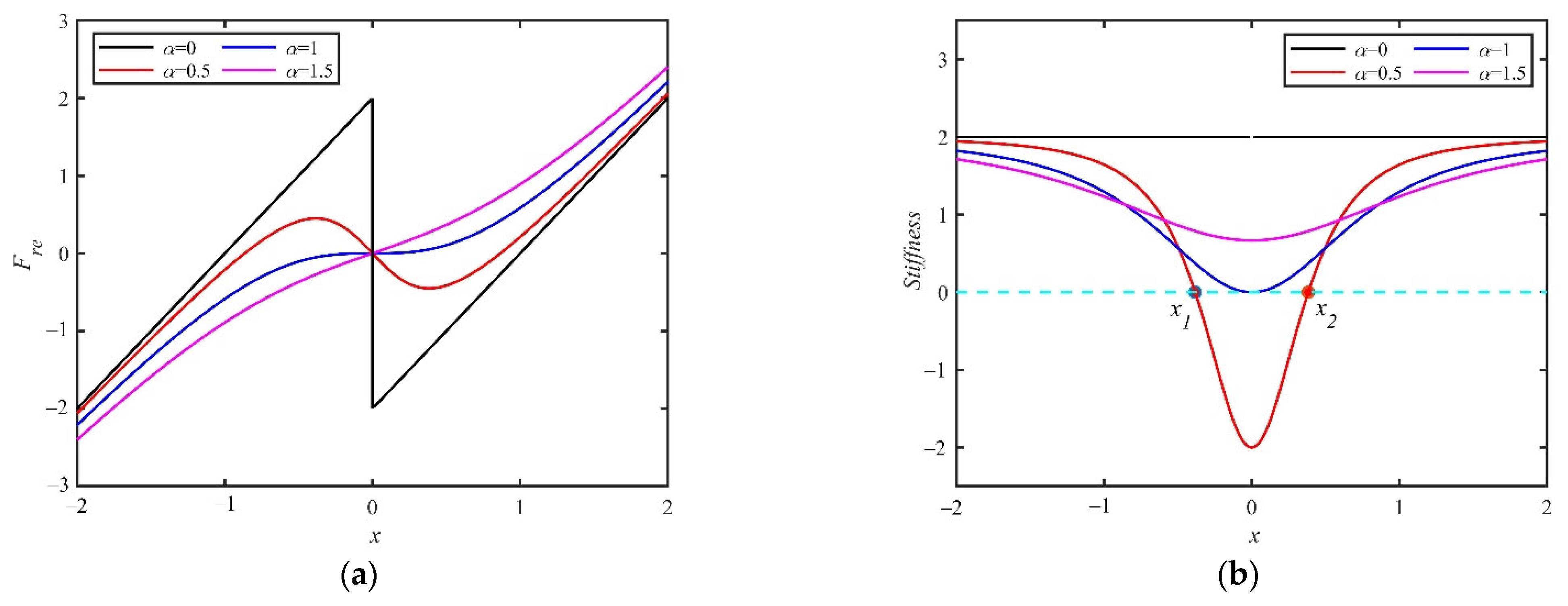
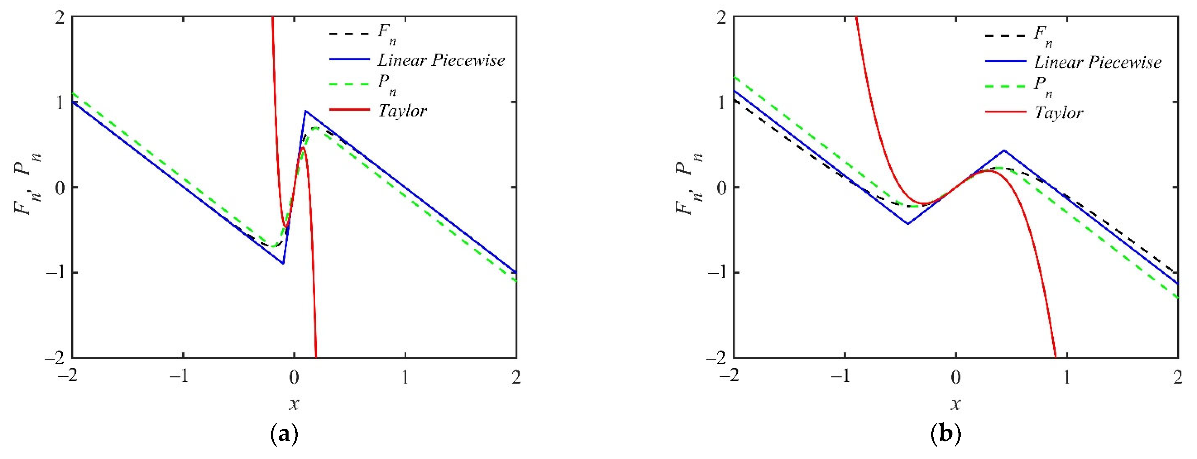
  • The nonlinear restoring force is accurately represented by the piecewise nonlinear function. The nonlinear characteristics of the restoring force in the interval x 0 < x < x 0 are retained, so that some novel nonlinear phenomena are found.
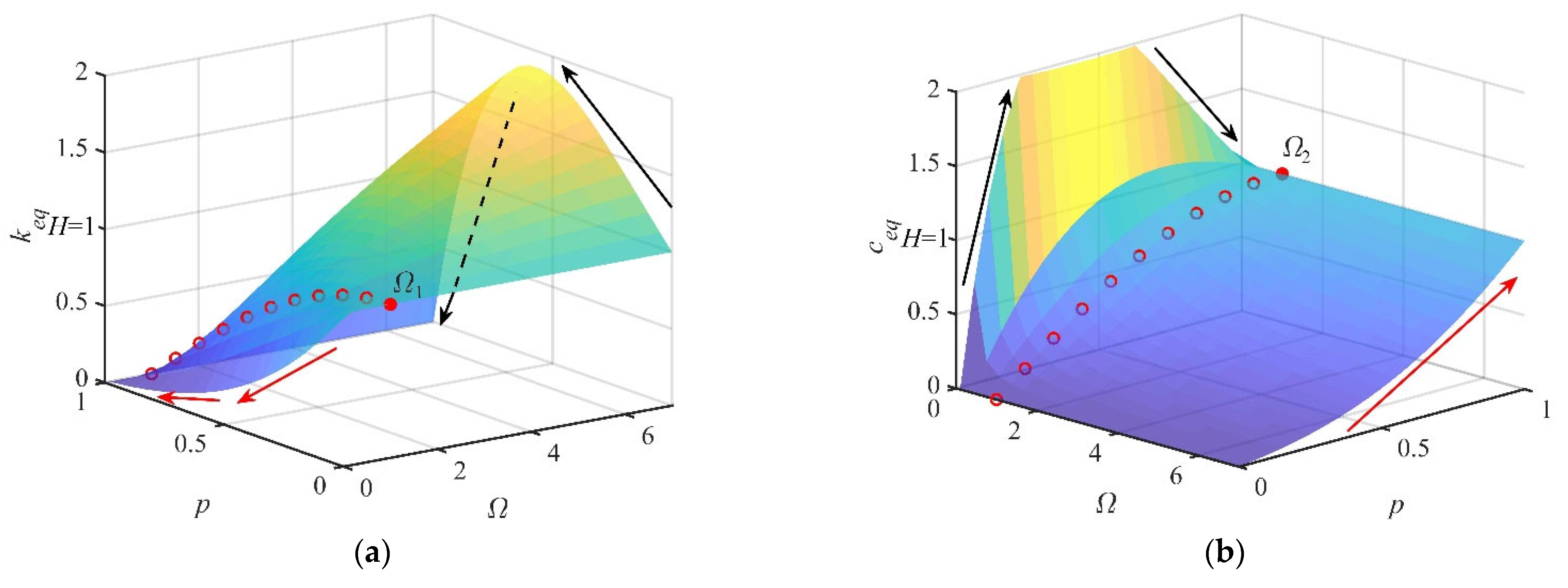
  • The orthogonal function is used to calculate the equivalent fractional coefficients. The equivalent stiffness coefficient and the equivalent damping coefficient are variable with respect to the p th and the ( p 1 ) th power of the excitation frequency. In the high-frequency region, the stiffness characteristic of the fractional model is dominant. The stiffness characteristic increases first and then decreases as the fractional order increases. In the low-frequency region, the damping characteristic of the fractional model is dominant. The damping characteristic increases first and then decreases as the fractional order increases. The fractional model affects the stiffness property and the damping property, simultaneously.
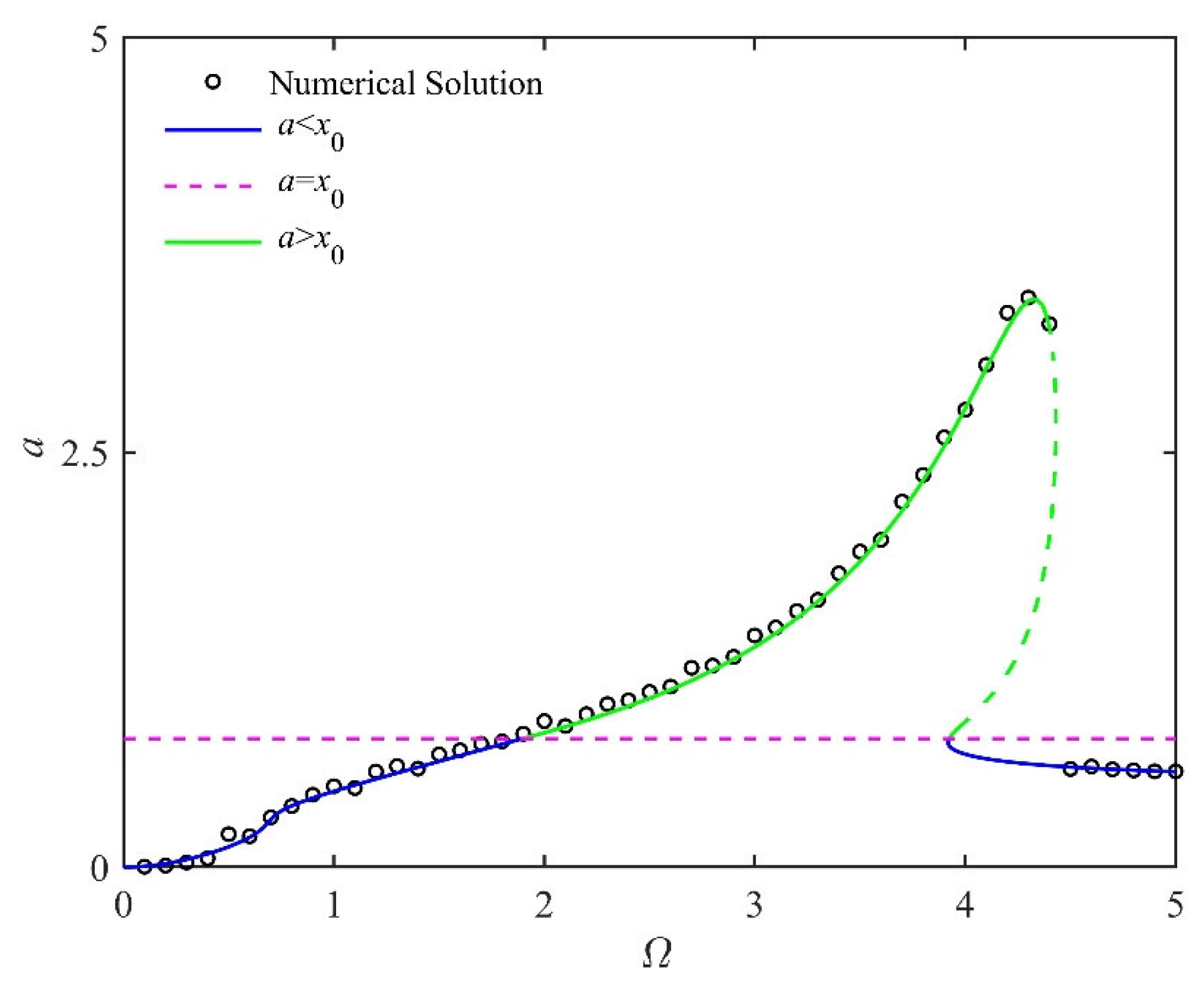
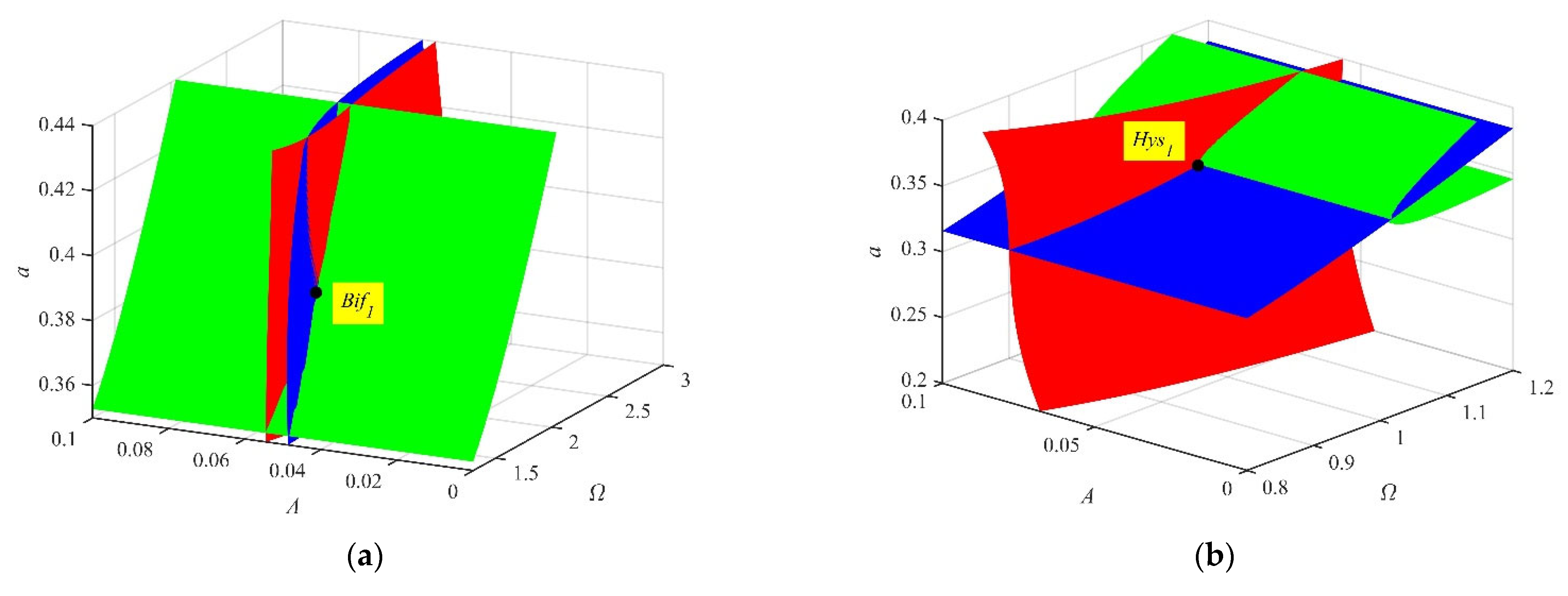
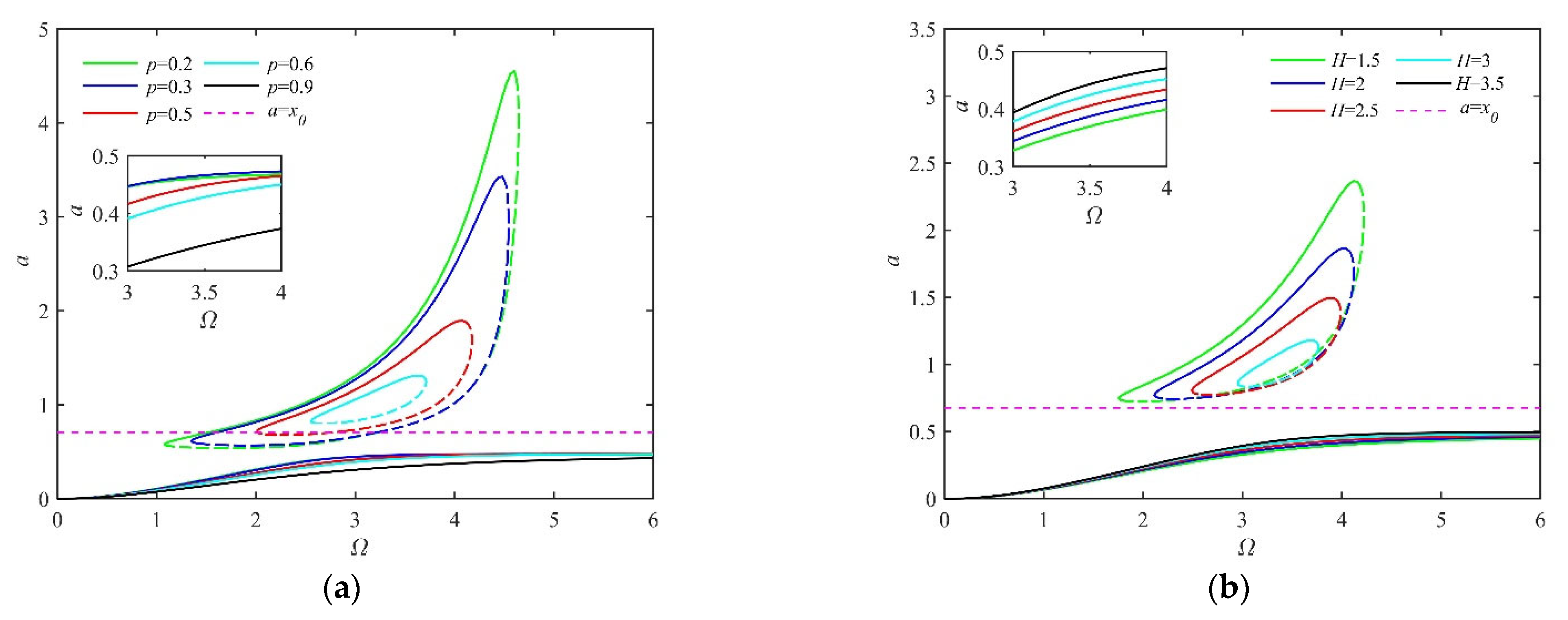
  • Based on the amplitude–frequency response functions, a novel transition process is found. With the decrease in the smooth parameter, the nonlinearity of the system increases. A hysteresis point appears first, followed by a bifurcation point and a frequency island. There are three attractors (two stable attractors and one unstable attractor) in the frequency island. In addition, the variation in the number and the stable state of attractors means that pitchfork bifurcation and transcritical bifurcation are found. It is rare that the vibration amplitude of the system can be changed in the entire resonant region because of the frequency island.
  • As the fractional parameters increase, the hysteresis point moves to the high-frequency and large-amplitude region, and the bifurcation point moves to the high-frequency and small-amplitude region. The frequency interval of the frequency island shortens. Finally, the frequency island disappears because the stable attractor and the unstable attractor collide.
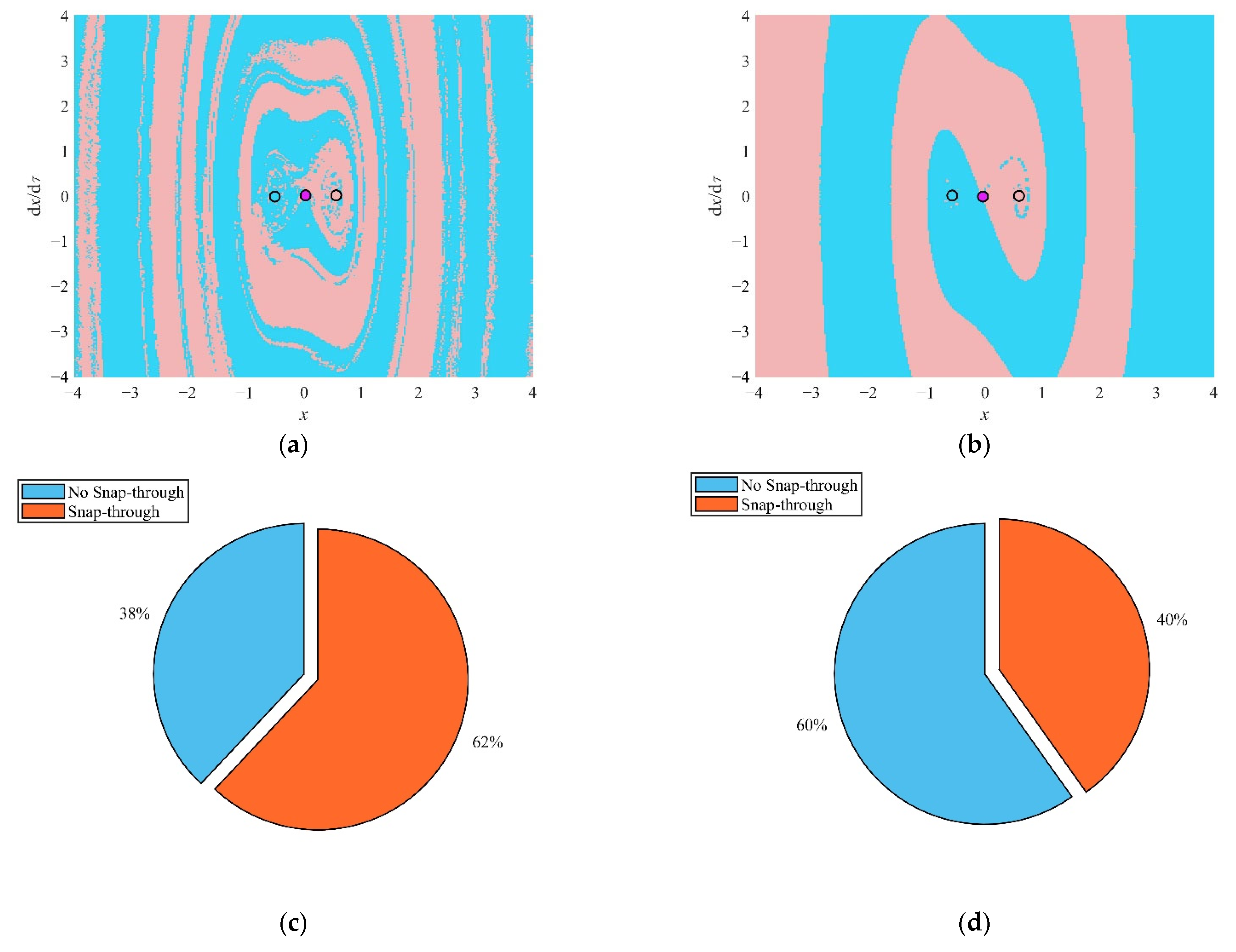
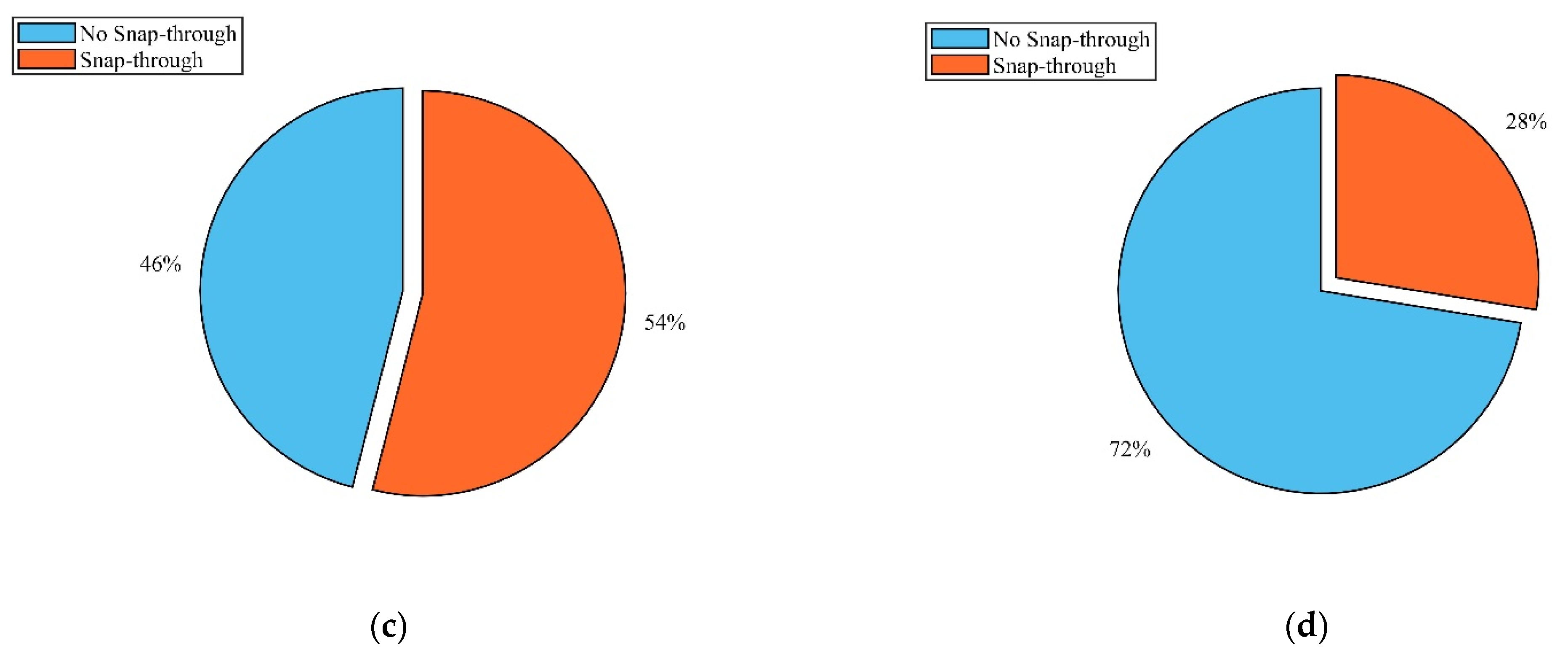
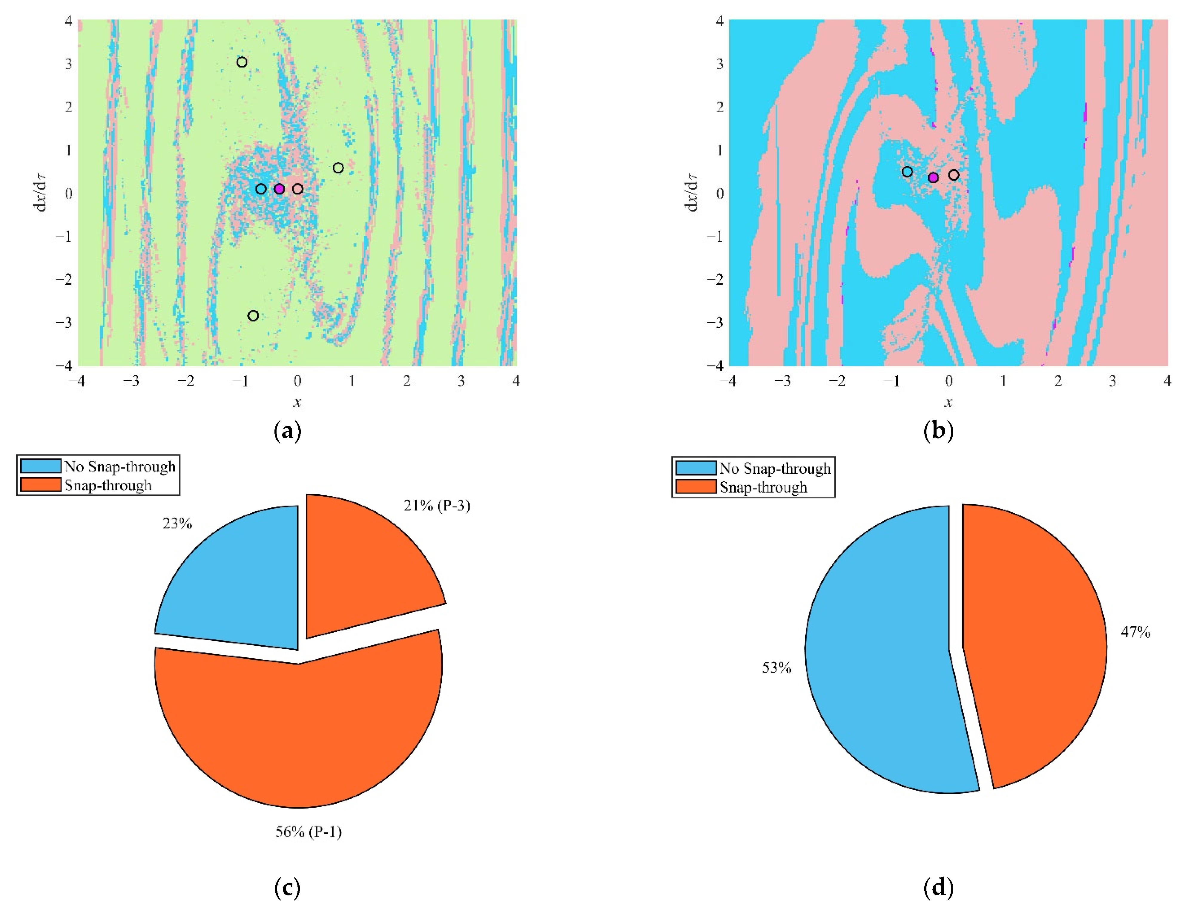
  • In the non-resonant region, the increase in the fractional parameters leads to the probability of the snap-through decreasing and the asymptotic stability of the steady-state solution increasing. When the excitation frequency is smaller than the natural frequency, the symmetry of the attraction domain enhances and the continuity increases. When the excitation frequency is larger than the natural frequency, the number of stable states of the system decreases. When the system is in a monostable state, no snap-through occurs.
Based on the above investigations, some novel nonlinear phenomena, such as a frequency island, of the SD oscillator with nonlinear fractional damping are revealed. This investigation may provide a theoretical basis for applying SD oscillators in energy harvesting, vibration isolation, and many other fields. In the future, some vibration isolation experiments and theoretical investigations for fractional SD oscillators utilizing the novel frequency island phenomenon may be useful for ultra-low-frequency vibration isolators.

Author Contributions

Conceptualization, M.W. and E.C.; methodology, M.W.; software, M.W.; validation, E.C., R.T. and C.W.; formal analysis, M.W.; investigation, M.W.; resources, E.C.; data curation, E.C.; writing—original draft preparation, M.W.; writing—review and editing, E.C. and R.T.; visualization, M.W.; supervision, E.C.; project administration, E.C.; funding acquisition, E.C. All authors have read and agreed to the published version of the manuscript.

Funding

This research was funded by the National Natural Science Foundation of China, grant number 12072205 and the Natural Science Foundation of Hebei Province, grant number A2022210024.

Institutional Review Board Statement

Not applicable.

Informed Consent Statement

Not applicable.

Data Availability Statement

Not applicable.

Acknowledgments

Thanks to the State Key Laboratory of Mechanical Behavior and System Safety of Traffic Engineering Structures.

Conflicts of Interest

The authors declare no conflict of interest.

Appendix A

R 11 = 2 ζ Ω + H Ω p sin p π 2 / 2 Ω
R 12 = a ¯ 4 3 a ¯ 2 B 2 K 0 + K 3 + 4 B 4 K 0 + K 1 Ω 2 + 4 H Ω p cos p π 2 / 2 Ω
R 13 = 9 a ¯ 2 B 2 K 0 + K 3 + 4 B 4 K 0 + K 1 Ω 2 + 4 H Ω p cos p π 2 / 8 π
R 14 = a ¯ 2 ζ Ω + H Ω p sin p π 2 / 2 π
R 21 = 1 2 Ω K 0 π 2 B 1 + x 0 1 x 0 a ¯ 2 + K 0 π 2 B 5 + x 0 1 x 0 a ¯ 2 K 0 x 0 2 π 1 x 0 a ¯ 2 3 a ¯ 2 B 2 + 4 B 4 2 B 2 x 0 2
+ a ¯ 2 2 π K 0 acos x 0 a ¯ + a ¯ 2 π 3 a ¯ 2 B 2 + 4 B 4 K 0 asin x 0 a ¯ + a ¯ K 1 + 3 4 a ¯ 3 K 3 a ¯ Ω 2 + a ¯ H Ω p cos p π 2
R 22 = 2 a ¯ 2 K 0 x 0 18 a ¯ 4 B 2 K 0 x 0 8 a ¯ 2 B 4 K 0 x 0 8 B 1 K 0 x 0 2 + 8 B 5 K 0 x 0 2 + 8 K 0 x 0 3 + 6 a ¯ 2 B 2 K 0 x 0 3 8 B 4 K 0 x 0 3
4 B 2 K 0 x 0 5 + 4 a ¯ 3 K 1 π 1 x 0 a ¯ 2 + 9 a ¯ 5 K 3 π 1 x 0 a ¯ 2 4 a ¯ 3 π 1 x 0 a ¯ 2 Ω 2 + 2 a ¯ 3 K 0 1 x 0 a ¯ 2 acos x 0 a ¯
+ 2 a ¯ 3 9 a ¯ 2 B 2 + 4 B 4 K 0 1 x 0 a ¯ 2 asin x 0 a ¯ + 4 a ¯ 3 H π 1 x 0 a ¯ 2 Ω p cos p π 2 / 8 a ¯ 3 π 2 1 x 0 a ¯ 2

Appendix B

G ˜ a = 4 K 1 + 3 a 2 K 3 + K 0 6 6 / α 2 / 3 + 3 a 2 α 4 / 3 α 2 / 3 / 2 1 + α 2 / 3 α 8 / 3 4 Ω 2 + 4 H Ω p cos p π / 2  
G Ω = 4 f 2 Ω 3 L 2 + 2 a 2 a ζ + a H p Ω p 1 sin p π 2 2 ζ Ω + H Ω p sin p π 2 + a 2 8 8 Ω + 4 H p Ω p 1 cos p π 2 G ˜ a
a < x 0 :
G = f 2 Ω 4 L 2 + 1 16 a 2 3 a 2 K 3 + K 0 α 4 / 3 α 2 / 3 2 1 + α 2 / 3 α 8 / 3 + 4 K 1 + 3 K 0 1 + α 2 / 3 2 α 2 / 3 Ω 2 + 4 H Ω p cos p π 2 2 + 2 a ζ Ω + a H Ω p sin p π 2 2
G a = a 8 6 a 2 K 3 + K 0 α 4 / 3 α 2 / 3 2 1 + α 2 / 3 α 8 / 3 G ˜ a + 16 2 ζ Ω + H Ω p sin p π 2 2 G ˜ a 2
G a a = 1 8 3 a 2 2 K 3 1 + α 2 / 3 α 8 / 3 + K 0 α 4 / 3 + α 2 / 3 8 3 K 0 α 4 / 3 + 2 + α 2 / 3 α 2 + 2 1 + α 2 / 3 α 2 K 1 Ω 2 9 a 2 2 K 3 α 2 / 3 α 4 / 3 + α 2 + K 0 1 + α 2 / 3 8 3 K 0 α 4 / 3 + 2 + α 2 / 3 α 2 + 2 1 + α 2 / 3 α 2 K 1 Ω 2 16 H 1 + α 2 / 3 a 2 Ω p cos p π 2 / 1 + α 2 / 3 2 a 14 / 3 + 16 2 ζ Ω + H Ω p sin p π 2 2 + 6 a 2 K 3 + K 0 α 4 / 3 α 2 / 3 2 1 + α 2 / 3 α 8 / 3 G ˜ a + G ˜ a 2
G Ω = 4 f 2 Ω 3 L 2 + 2 a 2 a ζ + a H p Ω p 1 sin p π 2 2 ζ Ω + H Ω p sin p π 2 + a 2 8 8 Ω + 4 H p Ω p 1 cos p π 2 G ˜ a
a > x 0 :
G = f 2 Ω 4 L 2 + 1 16 a 2 3 a 2 K 3 + K 0 α 4 / 3 α 2 / 3 2 1 + α 2 / 3 α 8 / 3 + 4 K 1 + 3 K 0 1 + α 2 / 3 2 α 2 / 3 Ω 2 + 4 H Ω p cos p π 2 2 + 2 a ζ Ω + a H Ω p sin p π 2 2
G a = 4 K 0 2 B 1 x 0 1 x 0 a 2 4 K 0 2 B 5 + x 0 1 x 0 a 2 + 2 K 0 x 0 1 x 0 a 2 3 a 2 B 2 + 4 B 4 + 2 B 2 x 0 2 8 a K 0 acos x 0 a 2 a 3 a 2 B 2 + 4 B 4 K 0 asin x 0 a a π 4 K 1 + 3 a 2 K 3 4 Ω 2 + 4 H Ω p cos p π 2 × 8 a 2 K 0 x 0 2 a 2 3 a 2 B 2 + 4 B 4 K 0 x 0 4 K 0 2 B 1 x 0 x 0 2 + 4 K 0 x 0 2 2 B 5 + x 0 12 a 2 B 2 K 0 x 0 a 2 x 0 2 2 K 0 x 0 3 3 a 2 B 2 + 4 B 4 + 2 B 2 x 0 2 + 8 a 3 K 0 1 x 0 a 2 acos x 0 a + 12 a 5 B 2 K 0 1 x 0 a 2 asin x 0 a + 2 a 3 3 a 2 B 2 + 4 B 4 K 0 1 x 0 a 2 asin x 0 a + a 3 π 1 x 0 a 2 4 K 1 + 9 a 2 K 3 4 Ω 2 + 4 H Ω p cos p π 2 / 8 a 3 π 2 1 x 0 a 2 + 2 a 2 ζ Ω + H Ω p sin p π 2 2
G a a = 1 x 0 a 2 8 a 2 K 0 x 0 18 a 4 B 2 K 0 x 0 8 a 2 B 4 K 0 x 0 8 B 1 K 0 x 0 2 + 8 B 5 K 0 x 0 2 + 8 K 0 x 0 3 + 6 a 2 B 2 K 0 x 0 3 8 B 4 K 0 x 0 3 4 B 2 K 0 x 0 5 + 4 a 3 K 1 π 1 x 0 a 2 + 9 a 5 K 3 π 1 x 0 a 2 4 a 3 π 1 x 0 a 2 Ω 2 + 8 a 3 K 0 1 x 0 a 2 acos x 0 a + 2 a 3 9 a 2 B 2 + 4 B 4 K 0 1 x 0 a 2 asin x 0 a + 4 a 3 H π 1 x 0 a 2 Ω p cos p π 2 2 4 a 3 π 1 x 0 a 2 Ω 2 + 8 a 3 K 0 1 x 0 a 2 acos x 0 a + 2 a 3 9 a 2 B 2 + 4 B 4 K 0 1 x 0 a 2 asin x 0 a + 4 a 3 H π 1 x 0 a 2 Ω p cos p π 2 2 a 3 1 x 0 a 2 12 a 2 K 1 π + 45 a 4 K 3 π 8 K 1 π x 0 2 36 a 2 K 3 π x 0 2 + 24 a K 0 x 0 1 x 0 a 2 90 a 3 B 2 K 0 x 0 1 x 0 a 2 24 a B 4 K 0 x 0 1 x 0 a 2 + 12 a B 2 K 0 x 0 3 1 x 0 a 2 12 a 2 π Ω 2 + 8 π x 0 2 Ω 2 + 8 K 0 3 a 2 2 x 0 2 acos x 0 a + 2 K 0 45 a 4 B 2 8 B 4 x 0 2 + 12 a 2 B 4 3 B 2 x 0 2 asin x 0 a + 12 a 2 H π Ω p cos p π 2 8 H π x 0 2 Ω p cos p π 2 4 K 0 2 B 1 x 0 1 x 0 a 2 4 K 0 2 B 5 + x 0 1 x 0 a 2 + 2 K 0 x 0 1 x 0 a 2 3 a 2 B 2 + 4 B 4 + 2 B 2 x 0 2 8 a K 0 acos x 0 a 2 a 3 a 2 B 2 + 4 B 4 K 0 asin x 0 a a π 4 K 1 + 3 a 2 K 3 4 Ω 2 + 4 H Ω p cos p π 2 + x 0 2 4 K 0 2 B 1 x 0 1 x 0 a 2 4 K 0 2 B 5 + x 0 1 x 0 a 2 + 2 K 0 x 0 1 x 0 a 2 3 a 2 B 2 + 4 B 4 + 2 B 2 x 0 2 8 a K 0 acos x 0 a 2 a 3 a 2 B 2 + 4 B 4 K 0 asin x 0 a
a π 4 K 1 + 3 a 2 K 3 4 Ω 2 + 4 H Ω p cos p π 2 8 a 2 K 0 x 0 2 a 2 3 a 2 B 2 + 4 B 4 K 0 x 0 4 K 0 2 B 1 x 0 x 0 2 + 4 K 0 x 0 2 2 B 5 + x 0 12 a 2 B 2 K 0 x 0 a 2 x 0 2 2 K 0 x 0 3 3 a 2 B 2 + 4 B 4 + 2 B 2 x 0 2 + 8 a 3 K 0 1 x 0 a 2 acos x 0 a + 12 a 5 B 2 K 0 1 x 0 a 2 asin x 0 a + 2 a 3 3 a 2 B 2 + 4 B 4 × K 0 1 x 0 a 2 asin x 0 a + a 3 π 1 x 0 a 2 4 K 1 + 9 a 2 K 3 4 Ω 2 + 4 H Ω p cos p π 2 + 3 a 2 x 0 2 4 K 0 2 B 1 x 0 1 x 0 a 2 4 K 0 2 B 5 + x 0 1 x 0 a 2 + 2 K 0 x 0 1 x 0 a 2 3 a 2 B 2 + 4 B 4 + 2 B 2 x 0 2 8 a K 0 acos x 0 a 2 a 3 a 2 B 2 + 4 B 4 K 0 asin x 0 a a π 4 K 1 + 3 a 2 K 3 4 Ω 2 + 4 H Ω p cos p π 2 8 a 2 K 0 x 0 2 a 2 3 a 2 B 2 + 4 B 4 K 0 x 0 4 K 0 2 B 1 x 0 x 0 2 + 4 K 0 x 0 2 2 B 5 + x 0 12 a 2 B 2 K 0 x 0 a 2 x 0 2 2 K 0 x 0 3 3 a 2 B 2 + 4 B 4 + 2 B 2 x 0 2 + 8 a 3 K 0 1 x 0 a 2 acos x 0 a + 12 a 5 B 2 K 0 1 x 0 a 2 asin x 0 a + 2 a 3 3 a 2 B 2 + 4 B 4 × K 0 1 x 0 a 2 asin x 0 a + a 3 π 1 x 0 a 2 4 K 1 + 9 a 2 K 3 4 Ω 2 + 4 H Ω p cos p π 2 + 16 a 6 π 2 1 x 0 a 2 3 / 2 2 ζ Ω + H Ω p sin p π 2 2 / 8 a 6 π 2 1 x 0 a 2 3 / 2

References

  1. Cao, Q.J.; Wiercigroch, M.; Pavlovskaia, E.E.; Grebogi, C.; Thompson, J.M.T. Archetypal oscillator for smooth and discontinuous dynamics. Phys. Rev. E 2006, 74, 046218. [Google Scholar] [CrossRef]
  2. Ashwani, K.P.; Nalin, A.C.; Dennis, S.B.; Sanjay, P.B.; Anthony, M.W. Feedback stabilization of snap-through buckling in a preloaded two-bar linkage with hysteresis. Int. J. Nonlinear Mech. 2007, 43, 277–291. [Google Scholar]
  3. Yang, T.; Liu, J.Y.; Cao, Q.J. Response analysis of the archetypal smooth and discontinuous oscillator for vibration energy harvesting. Phys. A Stat. Mech. Its Appl. 2018, 507, 358–373. [Google Scholar] [CrossRef]
  4. Hao, Z.F.; Cao, Q.J.; Wiercigroch, M. Two-sided damping constraint control for high-performance vibration isolation and end-stop impact protection. Nonlinear Dyn. 2016, 86, 2129–2144. [Google Scholar] [CrossRef]
  5. Avramov, K.V.; Mikhlin, Y.V. Snap-through truss as a vibration absorber. J. Vib. Control 2004, 10, 291–308. [Google Scholar] [CrossRef]
  6. Brennan, M.J.; Elliott, S.J.; Bonello, P.; Vincent, J.F.V. The “click” mechanism in dipteran flight: If it exists, then what effect does it have? J. Theor. Biol. 2003, 224, 205–213. [Google Scholar] [CrossRef]
  7. Ichiro, A.; Nakazawa, M. Non-linear dynamic behavior of multi-folding microstructure systems based on origami skill. Int. J. Non-Linear Mech. 2010, 45, 337–347. [Google Scholar]
  8. Waite, J.J.; Virgin, L.N.; Wiebe, R. Competing responses in a discrete mechanical system. Int. J. Bifurc. Chaos 2014, 24, 1430003. [Google Scholar] [CrossRef]
  9. Hao, Z.F.; Cao, Q.J. The isolation characteristics of an archetypal dynamical model with stable-quasi-zero-stiffness. J. Sound Vib. 2015, 340, 61–79. [Google Scholar] [CrossRef]
  10. Hao, Z.F.; Cao, Q.J. A novel dynamical model for GVT nonlinear supporting system with stable-quasi-zero-stiffness. J. Theor. Appl. Mech. 2014, 52, 199–213. [Google Scholar]
  11. Currier, T.M.; Lheron, S.; Modarres-Sadeghi, Y. A bio-inspired robotic fish utilizes the snap-through buckling of its spine to generate accelerations of more than 20 g. Bioinspir. Biomim. 2020, 15, 055006. [Google Scholar] [CrossRef]
  12. Ding, H.; Chen, L.Q. Designs, analysis, and applications of nonlinear energy sinks. Nonlinear Dyn. 2020, 100, 3061–3107. [Google Scholar] [CrossRef]
  13. Geng, X.F.; Ding, H.; Mao, X.Y.; Chen, L.Q. Nonlinear energy sink with limited vibration amplitude. Mech. Syst. Signal Process. 2021, 156, 107625. [Google Scholar] [CrossRef]
  14. Jiang, W.A.; Chen, L.Q. Snap-through piezoelectric energy harvesting. J. Sound Vib. 2014, 333, 4314–4325. [Google Scholar] [CrossRef]
  15. Speciale, A.; Ardito, R.; Marco, B.; Ferrari, M.; Ferrari, V.; Frangi, A.A. Snap-through buckling mechanism for frequency-up conversion in piezoelectric energy harvesting. Appl. Sci. 2020, 10, 3614. [Google Scholar] [CrossRef]
  16. Myongwon, H.; Andres, F. Topological wave energy harvesting in bistable lattices. Smart Mater. Struct. 2022, 31, 015021. [Google Scholar]
  17. Tan, D.G.; Zhou, J.X.; Wang, K.; Zhao, X.; Wang, Q.; Xu, D. Bow-type bistable triboelectric nanogenerator for harvesting energy from low-frequency vibration. Nano Energy 2022, 92, 106746. [Google Scholar] [CrossRef]
  18. Cao, Q.J.; Wiercigroch, M.; Pavlovskaia, E.E.; Thompson, J.M.T.; Grebogi, C. Piecewise linear approach to an archetypal oscillator for smooth and discontinuous dynamics. Philos. Trans. R. Soc. A Math. Phys. Eng. Sci. 2008, 366, 635–652. [Google Scholar] [CrossRef]
  19. Tian, R.L.; Cao, Q.J.; Li, Z.X. Hopf bifurcations for the recently proposed smooth-and-discontinuous oscillator. Chin. Phys. Lett. 2010, 27, 074701. [Google Scholar]
  20. Tian, R.L.; Cao, Q.J.; Yang, S.P. The codimension-two bifurcation for the recent proposed SD oscillator. Nonlinear Dyn. 2010, 59, 19–27. [Google Scholar] [CrossRef]
  21. Cao, Q.J.; Wiercigroch, M.; Pavlovskaia, E.E.; Grebogi, C.; Thompson, J.M.T. The limit case response of the archetypal oscillator for smooth and discontinuous dynamics. Int. J. Non-Linear Mech. 2008, 43, 462–473. [Google Scholar] [CrossRef]
  22. Shen, J.; Li, Y.; Du, Z. Subharmonic and grazing bifurcations for a simple bilinear oscillator. Int. J. Non-Linear Mech. 2014, 60, 70–82. [Google Scholar] [CrossRef]
  23. Han, Y.W.; Cao, Q.J.; Chen, Y.S.; Wiercigroch, M. A novel smooth and discontinuous oscillator with strong irrational nonlinearities. Sci. China Phys. Mech. Astron. 2012, 55, 1832–1843. [Google Scholar] [CrossRef]
  24. Cao, Q.J.; Han, Y.W.; Liang, T.W.; Wiercigroch, M.; Piskarev, S. Multiple buckling and codimension-three bifurcation phenomena of a nonlinear oscillator. Int. J. Bifurc. Chaos 2014, 24, 1430005. [Google Scholar] [CrossRef]
  25. Han, Y.W.; Cao, Q.; Chen, Y.S.; Wiercigroch, M. Chaotic thresholds for the piecewise linear discontinuous system with multiple well potentials. Int. J. Non-Linear Mech. 2015, 70, 145–152. [Google Scholar] [CrossRef]
  26. Han, Y.W.; Cao, Q.J.; Ji, J. Nonlinear dynamics of a smooth and discontinuous oscillator with multiple stability. Int. J. Bifurc. Chaos 2015, 25, 1530038. [Google Scholar] [CrossRef]
  27. Tian, R.L.; Wu, Q.L.; Yang, X.W.; Si, C.D. Chaotic threshold for the smooth-and-discontinuous oscillator under constant excitations. Eur. Phys. J. Plus 2013, 128, 80–91. [Google Scholar] [CrossRef]
  28. Yue, X.L.; Xu, W.; Wang, L. Stochastic bifurcations in the SD (smooth and discontinuous) oscillator under bounded noise excitation. Sci. China Phys. 2013, 56, 1010–1016. [Google Scholar] [CrossRef]
  29. Santhosh, B.; Padmanabhan, C.; Narayanan, S. Numeric-analytic solutions of the smooth and discontinuous oscillator. Int. J. Mech. Sci. 2014, 84, 102–119. [Google Scholar] [CrossRef]
  30. Chen, H. Global analysis on the discontinuous limit case of a smooth oscillator. Int. J. Bifurc. Chaos 2016, 26, 1650061. [Google Scholar] [CrossRef]
  31. Chen, H.B.; Jaume, L.; Tang, Y.L. Global dynamics of a SD oscillator. Nonlinear Dyn. 2018, 91, 1755–1777. [Google Scholar] [CrossRef]
  32. Wang, L.; Xue, L.; Xu, W.; Yue, X. Stochastic P-bifurcation analysis of a fractional smooth and discontinuous oscillator via the generalized cell mapping method. Int. J. Non-Linear Mech. 2017, 96, 56–63. [Google Scholar] [CrossRef]
  33. Chang, Y.J.; Chen, E.L.; Feng, M. Experimental study of the nonlinear dynamics of a smooth and discontinuous oscillator with different smoothness parameters and initial values. J. Theor. Appl. Mech. 2019, 57, 935–946. [Google Scholar] [CrossRef]
  34. Mainardi, F. Fractional relaxation-oscillation and fractional diffusion-wave phenomena. Chaos Solitons Fractals 1996, 7, 1461–1477. [Google Scholar] [CrossRef]
  35. Koeller, R.C. Applications of fractional calculus to the theory of viscoelasticity. J. Appl. Mech. 1984, 51, 299–307. [Google Scholar] [CrossRef]
  36. Caputo, M.; Mainardi, F. A new dissipation model based on memory mechanism. Pure Appl. Geophys. 1971, 91, 134–147. [Google Scholar] [CrossRef]
  37. Padovan, J.; Sawicki, J.T. Nonlinear vibrations of fractionally damped systems. Nonlinear Dyn. 1998, 16, 321–336. [Google Scholar] [CrossRef]
  38. Chang, Y.J.; Tian, W.W.; Chen, E.L.; Shen, Y.J.; Xing, W.C. Dynamic model for the nonlinear hysteresis of metal rubber based on the fractional-order derivative. J. Vib. Shock 2020, 39, 233–241. [Google Scholar]
  39. Caputo, M. Linear models of dissipation whose Q is almost frequency independent. Ann. Geophys. 1966, 19, 383–393. [Google Scholar] [CrossRef]
  40. Caputo, M. Linear model of dissipation whose Q is almost frequency independent-II. Geophys. J. Int. 2007, 13, 239–529. [Google Scholar] [CrossRef]
  41. Tarasov, V.E.; Zaslavsky, G.M. Dynamics with low-level fractionality. Phys. A Stat. Mech. Its Appl. 2006, 368, 399–415. [Google Scholar] [CrossRef] [Green Version]
Figure 1. (a) The prototypical SD oscillator model; (b) the schematic diagram of stable positions of the SD oscillator.
Fractalfract 06 00493 g001
Figure 2. (a) The nonlinear restoring force F r e ; (b) the stiffness of the SD oscillator; two points are x 1 = α α 2 / 3 1 and x 2 = α α 2 / 3 1 , respectively.
Fractalfract 06 00493 g002
Figure 3. The results of F n , P n , a linear piecewise function, and a three-order Taylor series equivalent function (a) α = 0.1 ; (b) α = 0.5 .
Fractalfract 06 00493 g003
Figure 4. The results of (a) the equivalent stiffness coefficient k e q ; (b) the equivalent damping coefficient c e q .
Fractalfract 06 00493 g004
Figure 5. The results of the amplitude-frequency response function and the numerical solution with ζ = 0.1443 , K 0 = 20 , K 1 = 1 , K 3 = 0.0256 , H = 1 , p = 0.5 , α = 0.9 , A = 0.08 .
Fractalfract 06 00493 g005
Figure 6. (a) The bifurcation set B i f 1 ; (b) the hysteresis set H y s 1 ; (c) the amplitude–frequency response curves; (d) the attractors and the attraction domain with α = 0.85 and Ω = 2.5 .
Fractalfract 06 00493 g006aFractalfract 06 00493 g006b
Figure 7. (a) The distribution of attractors in the frequency island; (b) the time history of vibration, the initial conditions of black line are selected as 0.5 , 0 , the initial conditions of red line are selected as 0.5 , 0.5 .
Fractalfract 06 00493 g007
Figure 8. (a) The distribution of attractors without the frequency island; (b) the time history of vibration, the initial conditions of black line, are selected as 1 , 0 , the initial conditions of red line are selected as 0 , 0 .
Fractalfract 06 00493 g008
Figure 9. The results of transition set with α = 0.89 ; (a) the hysteresis set with p = 0.37, 0.5, 0.7 and H = 1 ; (b) the hysteresis set of Equation (20) with H = 0.95, 1, 1.3 and p = 0.5 ; (c) the bifurcation set with p = 0.3, 0.5, 0.7 and H = 1 ; (d) the bifurcation set with H = 0.5, 1, 1.5 and p = 0.5 .
Fractalfract 06 00493 g009
Figure 10. The amplitude frequency response curves with (a) H = 1 , p = 0.2, 0.3, 0.5, 0.6 and 0.9; (b) p = 0.5 , H = 1.5, 2, 2.5, 3 and 3.5.
Fractalfract 06 00493 g010
Figure 11. The distribution of attractors in the frequency island with parameters are set as Ω = 3, H = 2 (a) p = 0.2 , (b) p = 0.5 , (c) p = 0.625 and (d) p = 0.7 .
Fractalfract 06 00493 g011
Figure 12. The distribution of attractors in the frequency island with parameters are set as Ω = 3, p = 0.7 (a) H = 1.5, (b) H = 2.5, (c) H = 3 and (d) H = 3.5.
Fractalfract 06 00493 g012
Figure 13. The distribution of attractors with the parameters are set as Ω = 1, H = 1 (a) p = 0 , and (b) p = 0.99 , and the probability of the snap-through with (c) p = 0 and (d) p = 0.99 .
Fractalfract 06 00493 g013
Figure 14. The distribution of attractors with the parameters are set as Ω = 1, p = 0.5 (a) H = 1, (b) H = 4, and the probability of the snap-through with (c) H = 1 and (d) H = 4.
Fractalfract 06 00493 g014aFractalfract 06 00493 g014b
Figure 15. The distribution of attractors with the parameters are set as Ω = 8.5, H = 1 (a) p = 0.1 , (b) p = 0.99 , and the probability of the snap-through with (c) p = 0.1 and (d) p = 0.99 .
Fractalfract 06 00493 g015
Figure 16. The distribution of attractors with the parameters are set as Ω = 8.5, p = 0.5 (a) H = 1, (c) H = 3, (e) H = 4; (b,d,f) are the diagrams of the probability of the snap-through with H = 1, 3 and 4, respectively.
Fractalfract 06 00493 g016
Publisher’s Note: MDPI stays neutral with regard to jurisdictional claims in published maps and institutional affiliations.

