Article

FOPI/FOPID Tuning Rule Based on a Fractional Order Model for the Process

1
Instituto de Investigaciones en Ingeniería, Facultad de Ingeniería, Universidad de Costa Rica, San José 11501-2060, Costa Rica
2
Curtin Centre for Optimisation and Decision Science, Curtin University, Bentley, WA 6102, Australia
3
Dipartimento di Ingegneria Meccanica e Industriale, Università degli Studi di Brescia, Via Branze 38, 25213 Brescia, Italy
4
Departament de Telecomunicació i d’Enginyeria de Sistemes, Escola d’Enginyeria, Universitat Autònoma de Barcelona, Bellaterra, 08193 Barcelona, Spain
*
Authors to whom correspondence should be addressed.
Fractal Fract. 2022, 6(9), 478; https://doi.org/10.3390/fractalfract6090478
Submission received: 22 July 2022 / Revised: 24 August 2022 / Accepted: 25 August 2022 / Published: 29 August 2022
(This article belongs to the Special Issue Advances in Fractional-Order PID Controllers)

Abstract

:
This paper deals with the design of a control system based on fractional order models and fractional order proportional-integral-derivative (FOPID) controllers and fractional-order proportional-integral (FOPI) controllers. The controller design takes into account the trade-off between robustness and performance as well as the trade-off between the load disturbance rejection and set-point tracking tasks. The fractional order process model is able to represent an extensive range of dynamics, including over-damped and oscillatory behaviors and this simplifies the process modelling. The tuning of the FOPID and FOPI controllers is achieved by using an optimization, as a first step, and in a second step, several fitting functions were used to capture the behavior of the optimal parameters of the controllers. In this way, a new set of tuning rules called FOMCoRoT (Fractional Order Model and Controllers Robust Tuning) is obtained for both FOPID and FOPI controllers. Simulation examples show the effectiveness of the proposed control strategy based on fractional calculus.

1. Introduction

Theoretical and practical studies have demonstrated the advantages of using fractional calculus in the modelling and control of dynamic systems, mainly from an industrial process control point of view [1,2]. For instance, in process modelling, several works (see, for example [3,4,5,6,7,8,9,10,11]) have shown that fractional order models with one or two fractional parameters can represent the process dynamics better than integer transfer functions of low order, such as the well-known first order plus dead time (FOPDT) and second order plus dead time (SOPDT) models. Therefore, a wider range of real-world processes can be modeled and an improved control system design can be achieved.
In particular, this paper considers a fractional first order plus dead time (FFOPDT) model that is able to represent a wide range of dynamics, including non-oscillatory, as the typical first order and oscillatory ones, as those exhibited by under-damped processes. Moreover, the effectiveness of this model has been proved through research (see for example [12,13,14,15,16]). This model is useful in practice because it addresses a frequent shortcoming of tuning rules available in the literature, that is, they are based on a specific low-order integer transfer function, such that they can only be applied to a restricted range of dynamics. Thanks to this feature of the FFOPDT model, it is not necessary to change the method used to tune the integer or non-integer controller, because the structure of the model remains the same irrespective of the over- or under-damped nature of the process.
Another interesting application of fractional calculus is the design of the control algorithm. It has been demonstrated that the fractional proportional-integral-derivative (FOPID) controllers provide more flexibility and accuracy in the adjustment of the feedback system. This can be used to guarantee more stringent specifications related to relative stability—phase, gain margins, and maximum sensitivity—and performance—set-point tracking and load-disturbance rejection—in comparison to those achievable with the classical PID controller (see, for instance [3,5,6,17,18,19]).
In the literature, different approaches to tune FOPID controllers have been devised. Some of them take into account the robustness of the control system with respect to process variations and model uncertainty, and therefore specifications such as gain crossover frequency, phase margin, or robustness to variations of the gain are imposed, see [3,5,20,21]; while others consider the maximum sensitivity index M S as a measure of robustness, as in [6,16,22,23,24,25].
Other approaches have applied artificial intelligence based on fuzzy logic control to adjust the FOPID controller parameters [7,17,26], while others focus exclusively on integral performance criteria as in [27].
Finally, some approaches take into consideration the robustness and the performance of the closed-loop system at the same time; among them, ref [28] optimizes the load-disturbance rejection, ref [29] minimises an objective function in the frequency response, and [18] considers either an optimal performance for set-point tracking task or for load-disturbance rejection.
Despite the wealth of results available in the literature, it is difficult to find a set of rules that consider the trade-off between performance and robustness, and between the set-point tracking task, also known as servo-control operation, and load-disturbance rejection, also known as regulatory-control mode. To overcome these limitations, in this paper we propose a new approach, the FOMCoRoT, to design fractional-order PID and PI controllers. The main novelty of the proposed method is that it explicitly considers the above mentioned trade-offs and uses an FFOPDT model, thereby taking advantage of both a fractional controller and the flexibility of a fractional model. Furthermore, given the considered fractional-order process model, the devised tuning rules are also more general than those found in the literature.
This paper is organized as follows. Section 2 is devoted to the problem formulation, the description of the process model, as well as of the control algorithm and of the performance and robustness indices. Section 3 focuses on the design of the FOMCoRoT method for FOPID and FOPI controllers. An analysis of the robustness and performance is presented in Section 4 and bounds are established to decide when the use of fractional controllers is recommended to guarantee a minimum improvement of the performance compared to the one obtainable with classical PID/PI controllers. Then, in Section 5, simulation examples with the corresponding results are presented. Finally, conclusions are drawn in Section 6.

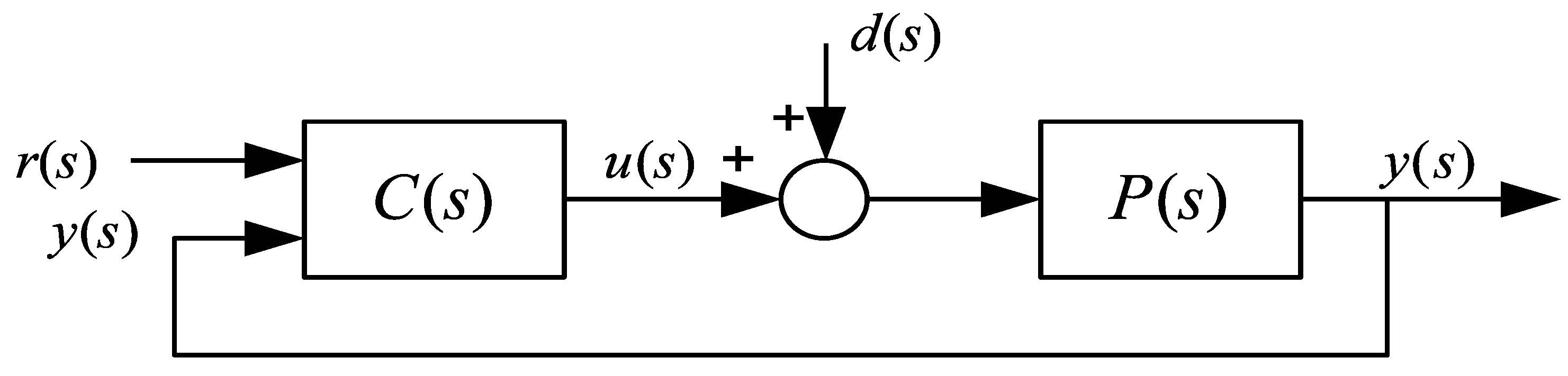
2. Problem Formulation

In order to obtain the tuning rule for FOPI/FOPID controllers, we consider the closed-loop control system shown in Figure 1, where P ( s ) is the controlled process model and C ( s ) the controller to be tuned. In this system, r ( s ) , u ( s ) , d ( s ) , and y ( s ) , are the set-point signal, the controller output, the load-disturbance, and the feedback signal, respectively.

2.1. Controlled Process Model

The controlled process is a Fractional First Order Plus Dead Time model, referred here as a FFOPDT model, whose dynamic is described by the following transfer function:
P ( s ) = K e L s T s α + 1 ,
where K is the static gain, T is the time constant, L is the dead-time, and α is the fractional-order parameter. The FFOPDT dynamics are fully characterized by using two dimensionless parameters: the fractional order α and the normalized fractional dead-time τ 0 , defined as τ 0 = L T 1 α .
This model with values of α between 1 and 2 was selected because it can easily represent the most typical industrial processes with either over- or under-damped dynamics. In Figure 2, it can be seen how the fractional order α modifies the shape of the step response. It is important to highlight that when α = 1 , the classical FOPDT model is obtained, and when α = 2 a pair of pure imaginary poles are found (undamped oscillatory behavior).
When a fractional system is considered, the application of a rational approximation for the non-integer term is required. For this tuning rule design, the integer representation of the fractional term s α is obtained by applying the so-called CRONE approach [30], defined as:
s α s [ ω l , ω h ] α C o k = 1 N 1 + s w z , k 1 + s w p , k , α > 0 ,
where [ ω l , ω h ] (selected as [ 0.001 , 1000 ] in this work) is the frequency range where the approximation is valid and the term C o is adjusted so that the approximation has a unity gain at the logarithmic midpoint of the approximation range. Furthermore, the parameter N in (2) (in this case N = 8 to meet the minimum value N = l o g ( ω h ω l ) recommended by [30]) is used to select the number of poles and zeros of the real-rational transfer function that approximates the fractional term.

2.2. FOPI(D) Controller Equation

The output signal of the considered one-degree-of-freedom (1DoF) PI(D) controller is:
u ( s ) = K p e p ( s ) + e i ( s ) + e d ( s ) ,
with
e p ( s ) =   r ( s ) y ( s ) ,
e i ( s ) =   1 T i s λ [ r ( s ) y ( s ) ] ,
e d ( s ) =   T d s μ T d ζ s + 1 y ( s ) ,
where K p is the proportional gain, T i is the integral time, T d is the derivative time, and λ and μ are the fractional orders for the integral and derivative part, respectively. Moreover, T d ζ is the derivative filter time constant (traditionally selected by fixing ζ = 10 in integer PID controllers) [31]. In order to preserve the effectiveness of this parameter on the performance of the closed-loop system, mainly in the rejection of the high frequency noise and without changing the controller dynamics significantly, it was selected as:
ζ = 10 T d μ 1 μ ,
for FOPID controllers with the purpose of placing the pole corner frequency one decade after the zero frequency of the derivative action as it is often considered in the case of the series PID controller. Notice that an integer order filter has been included because, when using the CRONE approximation, this will be sufficient to guarantee the properness of the controller irrespective of the derivative order μ .
Finally, as shown in (6), the derivative action is only applied to the feedback signal, in order to avoid abrupt changes in the controller output signal, known as derivative kick, when a set-point step change occurs [32]. In the case of a FOPI controller, we simply set e d ( s ) = 0 .

2.3. Performance and Robustness

With the purpose of designing the tuning rule for the FOPI and FOPID controllers, the trade-off between performance and robustness has been considered along the lines of [33,34,35,36]. The function to be optimized is a multi-objective performance index given by:
J t = J e r + J e d ,
where J e r quantifies the set-point tracking performance and J e d measures the load-disturbance rejection performance. Both indices are computed as the integral of the absolute value of the error, given by:
J e = 0 e ( t ) d t = 0 r ( t ) y ( t ) d t .
The integral absolute error (IAE) is commonly used because, generally, it guarantees a low overshoot and a low settling time at the same time [37]. Note that the IAE index is finite only if λ 1 [38]. The design procedure is usually based on a low order model identified at the closed-loop operating point, thereby disregarding non-linearities, which are found in most of the real-world industrial processes. Therefore, it is critical to consider certain stability degree or robustness requirements. For these reasons, the devised tuning rule was obtained by minimising the integral absolute of the error (9), subject to a constraint imposed on the maximum value of the sensitivity function, which is defined as:
M S = max ω S ( j ω ) = max ω 1 1 + C ( j ω ) P ( j ω ) .
This index represents the inverse of the maximum distance of the Nyquist plot from the critical point ( 1 + j 0 ) and therefore provides a measure of the stability margin of the closed-loop system. The M S value should remain, at least for stable processes, in the range 1.4 M S 2.0 [32]. In this paper the limits of this range ( M S t = 1.4 and M S t = 2.0 ) are considered, where M S t denotes the target value of the maximum value of the magnitude of the sensitivity function.

3. Optimal Tuning

In order to find the optimal parameters for the FOPID controller, the range 1.0 α 1.8 for the fractional order α of the model has been considered. Note that for values of α greater than 1.8, the process becomes practically an undamped second order system which is rarely encountered in practical applications.
In the case of FOPI controllers, the fractional order α of the model in the range 1.0 α 1.6 has been established. This is because values of α greater than 1.6 leads to extremely low values of the normalized proportional gain κ p , which is in line with the long-held perception that PI regulators are unsuitable to control highly under-damped processes.
In both cases, the fractional order α was varied in steps of 0.1 and the normalized fractional dead-time τ 0 was considered in the range 0.1 τ 0 2.0 , in steps of 0.1. Note that such a range includes both lag-dominant and dead-time dominant processes for which (FO)PID controllers can achieve a reasonable performance. For larger values of the normalized dead time, more complex control structures, e.g., Smith predictor, should be used.
The optimal parameters for FOPI and FOPID controllers for both M S t = 1.4 and M S t = 2.0 were obtained by optimizing the cost function (8) constrained to M S = M S t , where the maximum sensitivity M S is defined in (10). To solve the optimization problem, the MATLAB© solver fminimax and the active-set algorithm were used. Once the optimal parameters were found, different fitting functions were used to obtain simple tuning rules based on the fractional order model (1).
As an example of how the tuning rule has been obtained, in Figure 3 the optimal values of the normalized proportional gain κ p have been plotted for different values of the normalized fractional dead-time τ 0 , as well as the corresponding interpolating function in the case of the FOPID controller.
As the final result, the following general structure for the normalized FOPID controller parameters has been devised:
κ p = K p K = a 1 τ 0 a 2 + a 3 ,
τ i = T i T λ α = b 1 τ 0 4 + b 2 τ 0 3 + b 3 τ 0 2 + b 4 τ 0 + b 5 ,
λ = 1 ,
τ d = T d T μ α = c 1 τ 0 3 + c 2 τ 0 2 + c 3 τ 0 + c 4 ,
μ = d 1 τ 0 3 + d 2 τ 0 2 + d 3 τ 0 + d 4 ,
Values of the constants are presented in Table 1 for M S t = 1.4 and in Table 2 for M S t = 2.0 .
In the case of the FOPI controller, the following general structure was devised:
κ p = K p K = a 1 τ 0 a 2 + a 3 ,
τ i = T i T λ α = b 1 τ 0 b 2 + b 3 ,
λ = c 1 τ 0 c 2 + c 3 .
Values of the constants are presented in Table 3 for M S t = 1.4 and in Table 4 for M S t = 2.0 . It is important to highlight that when the fractional order α of the model was also equal to one, the optimal value for the fractional term λ of the integral mode was also equal to one. The same happens for values of the normalized fractional dead-time τ 0 greater than 0.6 and M S t = 2.0 and therefore, in those cases, there is not any advantage in using a more complex structure for the controller as the FOPI. For that reason, the fitting functions presented in Equations (16)–(18) were limited to the mentioned range.

4. Robustness and Performance Analysis for the Tuning Rule

4.1. FOPID Controllers

For FOPID controllers, the devised tuning rule for κ p , τ i , τ d , λ , and μ are given by the expressions (11)–(15), where the values of the coefficients are presented in Table 1 for M S t = 1.4 and in Table 2 for M S t = 2.0 . Note that the optimal value for λ is always equal to one, and therefore the advantages in performance and robustness of using a FOPID controller are given by the fractional order μ associated with the derivative part. This is in line with the results shown in [18], where it was proven that the fractional order associated with the integral part did not provide any advantage when a FOPID controller is designed by minimizing the integral absolute error.
To show the effectiveness of the FOMCoRoT tuning rule, two aspects were evaluated. The first was the maximum sensitivity M S . The second was a comparison against the performance obtained with PID controllers designed by the same constraint on the maximum sensitivity and minimizing the same performance index (8). The optimal performance indexes for PID controllers, denoted by J t P I D , were taken from [39] and the J t performance index was obtained by applying the FOMCoRoT tuning rule developed in this work using FOPID controllers. For this comparison, the index η is defined as:
η = J t J t P I D ,
was used. Note that η less than one denotes and improvement in the performance provided by the tuning rule FOMCoRoT.
The evaluation of the maximum sensitivity value was made considering the fractional order α from 1.0 to 1.8 and the normalized fractional dead-time τ 0 from 0.1 to 2.0 , in steps of 0.05 for both parameters. The results are shown in Figure 4 for both M S t = 1.4 (blue surface) and M S t = 2.0 (yellow surface). As it can be seen in the figure, the maximum sensitivity has a stable behavior very close to the target one.
The index η for M S t = 1.4 in Figure 5 shows that the improvement in the performance provided by the use of a FOPID controllers is greater than 5 % (black dashed line in Figure 5) in two specific regions when 1.0 α 1.2 and 0.1 τ 0 1.3 , approximately, and when 1.7 α 1.8 . It is important to highlight that the first region encompasses most of the dynamics present in practical control applications, including first order and overdamped dynamics. In this region, the performance improvement achievable with the FOMCoRoT method can be as high as 10.5% larger than the one obtained with PID controllers. The second region comprises highly underdamped dynamics and, according to [40], for the fractional order range 1.7 α 1.8 the corresponding overshoot should roughly be between 53.2% and 67.2% and the improvement in the performance can reach 31.2%.
The index η for M S t = 2.0 is shown in Figure 6. As in the case M S t = 1.4 , some regions can be defined where the increase in the performance provided by the use of the FOMCoRoT method for FOPID over the optimal performance obtained with PID controllers is larger than or equal to 5%. The first region is characterized by α = 1.8 and τ 0 0.4 , and an improvement in the performance of up to 34% can be achieved. The second region is defined by α = 1.7 and τ 0 0.6 , and in this case, the improvement can reach values of 21%. The third region is for α = 1.6 and τ 0 1.2 , with an amelioration of up to 11% in the J t index.

4.2. FOPI Controllers

For FOPI controllers, the FOMCoRoT tuning rule for κ p , τ i , and λ are given by the expressions (16)–(18), where the values of the parameters are presented in Table 3 for M S t = 1.4 and in Table 4 for M S t = 2.0 . Note that the advantages in performance and robustness of using a FOPI controller are given by the fractional order λ associated to the integral part.
The evaluation of the maximum sensitivity was made considering the fractional order α from 1.1 to 1.6 and the normalized fractional dead-time τ 0 from 0.1 to 2.0 for M S t = 1.4 and from 0.1 to 0.6 for M S t = 2.0 , both parameters were varied in steps of 0.05. Note that these cover a wider range than the one used to devise the tuning rules. The results are shown in Figure 7. The maximum sensitivity index is very close to the target one.
To evaluate the performance obtained by applying the FOMCoRoT tuning along the line comparison carried out for FOPID controllers, it is defined the performance index:
η = J t J t P I ,
where J t P I is obtained from [39].
As expected, this index is always less or equal than one because an improvement in the performance of the closed-loop system is always obtained using a fractional controller.
The index η is shown in Figure 8 for M S t = 1.4 , where black dashed line delimits the regions where a 5% performance improvement can be achieved. The performance improvement for τ 0 in the interval [0.1 1.3] and α = 1.6 can be up to 24%; for τ 0 in the range [0.1 2.0] and α = 1.5 , up to 10%; for τ 0 in [0.1 0.4] and [1.3 2.0] and α = 1.4 , up to 14%; for τ 0 in [0.2 0.3] and [1.4 2.0] and α = 1.3 , up to 12%, and for τ 0 in [0.1 0.2] and α = 1.1 , up to 13%.
The performance analysis based on index η for FOPI controllers with M S t = 2.0 is shown in Figure 9. The interval where the performance improves by more than 5% is given by τ 0 ∈ [0.1 0.3] and α = 1.6 , and the improvement in performance can be up to 14%.

5. Simulation Examples

In order to demonstrate the effectiveness of the designed tuning rule FOMCoRoT, a high order process P 1 studied in [18] and shown in Equation (21), as well as a fractional order process P 2 studied in [16] and shown in Equation (22), are considered. All numerical simulations have been performed using MATLAB©.
P 1 = 1 ( s + 1 ) 8 , P m 1 = e 4.86 s 4.01 s 1.07 + 1 , P m 2 = e 4.95 s 3.06 s + 1 .
Consider the process P 1 . For the purpose of comparison, and in order to apply different tuning methods, two models were identified: a fractional order model P m 1 , by using the IDFOM tool [41], and the integer order model P m 2 that was considered in [18].
The accuracy of the model is evaluated by measuring the integral of the absolute value of the difference between the step response of the actual system P 1 and the model, P m 1 or P m 2 ( I A E m index). For P m 1 the I A E m index is equal to 0.6031 and for P m 2 it is equal to 0.5938 and therefore, in this example, the advantages of the fractional calculus in the robustness and performance of the closed-loop system due the controller’s algorithm will mainly be quantified.
Three methods were applied to tune the parameters of different structures of FOPID controllers. The technique proposed in [18] (referred here as P.&V. SP for set-point tracking or P.&V. LD for load-disturbance rejection) which considers a FOPID controller in series form and a FOPDT model, and aims at minimizing the integrated absolute error when a step change in the set-point or in the load-disturbance appears, with a constraint on the maximum sensitivity index. The second method proposed in [16], (referred here as H-F) uses series FOPID controller and a fractional order model as the one considered in this work, which aims for a trade-off performance in both set-point tracking and load-disturbance rejection, also considering the maximum sensitivity index as measure of robustness. The third approach is the FOMCoRoT method developed in this work. The results for performance and robustness are presented in Table 5 for M S t = 1.4 and M S t = 2.0 . As was mentioned above, in this work the derivative mode was only applied to the feedback signal in order to avoid extreme changes in the controller output when a step change in the set-point value is applied. However, for the sake of fair comparison, the tracking performance when the derivative action is applied to the error signal is also evaluated. To this end, the performance indexes J e r and J t are defined, similarly to J J e r and J t , respectively, but replacing y ( t ) with r ( t ) y ( t ) .
Figure 10 shows the closed-loop responses for both tasks: a step change in the set-point value and in the load-disturbance signal. It can be noted in Table 5 that, when the constraint on robustness is given by M S t = 1.4 , the best performance is achieved with the closed-loop system designed using the FOMCoRoT method ( J e d only has practically the same value in comparison with the one obtained by applying P.&V. LD). When the robustness is given by a nominal value M S t = 2.0 , the best performance in the feedback system is again provided by the FOMCoRoT method (only J e d is better with the H-F 2.0 method, but this can be attributed to a greater value of the maximum sensitivity index, M S = 2.8553 ). If the analysis is focused on the overall performance given by the indices J t or J t , the best performance is obtained by applying the FOMCoRoT method.
For the fractional order process P 2 two models were identified: a fractional order model P m 3 by applying the methodology proposed by [16] and an integer order model P m 4 obtained by applying the three points 123c identification method presented in [42].
P 2 = 1 s 2.6 + 2.2 s 1.5 + 2.9 s 1.3 + 3.32 s 0.9 + 1 , P m 3 = e 0.5171 s 6.8601 s 1.0413 + 1 , P m 4 = e 0.655 s 5.406 s + 1 .
The model accuracy was also evaluated through the I A E m index. For P m 3 the I A E m index is equal to 0.7557 and for P m 4 it is equal to 0.2566. It can be noted that the fractional model provides a lower accuracy than the integer model. This is because, despite the increased flexibility of the fractional model, different identification methods yield different results. In any case, the fractional model is sufficiently accurate to be used effectively with the FOMCoRoT tuning rules.
In Table 6, the performance indexes when step changes appear in the set-point and in the load-disturbance values are presented. It can be noted that the best performance for each operation mode (measured with the J e r or J e d index) and for the overall performance ( J t index) is obtained when the controller parameters are tuned with the FOMCoRoT method. This can be noted also in Figure 11.

6. Conclusions

This paper deals with the design of a closed-loop control system using fractional order models and controllers. The procedure used to develop the FOMCoRoT method guarantees a suitable performance in both set-point tracking and load-disturbance rejection, because it has been designed to minimize a combined performance index that takes into account both operation modes. Moreover, the tuning rule designed in this work provides guaranteed stability margins due to a constraint in the control system robustness obtained by imposing suitable values for the maximum sensitivity index M S .
Through performance analysis and simulation results, it can be concluded that FOPID and FOPI controllers provide a major impact in the closed-loop system performance when a high degree of robustness is required.
Two simulation examples have shown the effectiveness of the FOMCoRoT method in combination with a FFOPDT model, and this work will allow the user to have a systematic method to decide whether it is suitable to use the fractional calculus to design the control system for a given application or not.
Finally, it is worth pointing out that the proposed method deals with the design of industrial controllers, but other research lines such as controllability, observability, optimal control, robust control, etc. should be pursued in fractional order control systems in order to have a complete theoretical framework for these systems, and in particular an understanding of how the fractional order impacts the above-mentioned structural properties of a system.

Author Contributions

Conceptualization, H.M., O.A., F.P., A.V. and R.V.; Data curation, H.M. and O.A.; Formal analysis, H.M., O.A., F.P., A.V. and R.V.; Funding acquisition, O.A. and R.V.; Investigation, H.M., O.A., F.P., A.V. and R.V.; Methodology, H.M. and O.A.; Software, H.M.; Project administration, O.A.; Resources, O.A. and A.V.; Supervision, O.A. and R.V.; Validation, F.P. and A.V.; Writing—original draft, H.M. and O.A.; Writing—review and editing, F.P., A.V. and R.V. All authors have read and agreed to the published version of the manuscript.

Funding

This work has been supported by the Spanish CICYT program under grant PID2019-105434RB-C33. Also, the financial support from the University of Costa Rica, under the grant 731-B9-265, is greatly appreciated.

Institutional Review Board Statement

Not applicable.

Informed Consent Statement

Not applicable.

Data Availability Statement

Not applicable.

Conflicts of Interest

The authors declare no conflict of interest.

References

  1. Tepljakov, A.; Alagoz, B.B.; Yeroglu, C.; Gonzalez, E.A.; Hosseinnia, S.H.; Petlenkov, E.; Ates, A.; Cech, M. Towards Industrialization of FOPID Controllers: A Survey on Milestones of Fractional-Order Control and Pathways for Future Developments. IEEE Access 2021, 9, 21016–21042. [Google Scholar] [CrossRef]
  2. Dastjerdi, A.A.; Vinagre, B.M.; Chen, Y.; HosseinNia, S.H. Linear fractional order controllers; A survey in the frequency domain. Annu. Rev. Control 2019, 47, 51–70. [Google Scholar] [CrossRef]
  3. Malek, H.; Luo, Y.; Chen, Y. Identification and tuning fractional order proportional integral controllers for time delayed systems with a fractional pole. Mechatronics 2013, 23, 746–754. [Google Scholar] [CrossRef]
  4. Königsmarková, J.; Čech, M. Robust PI/PID parameter surfaces for a class of fractional-order processes. IFAC-PapersOnLine 2018, 51, 763–768. [Google Scholar] [CrossRef]
  5. Zhao, C.; Xue, D.; Chen, Y. A fractional order PID tuning algorithm for a class of fractional order plants. In Proceedings of the IEEE International Conference Mechatronics and Automation, Niagara Falls, ON, Canada, 20 July–1 August 2005; Volume 1, pp. 216–221. [Google Scholar] [CrossRef]
  6. Li, D.; Liu, L.; Jin, Q.; Hirasawa, K. Maximum sensitivity based fractional IMC–PID controller design for non-integer order system with time delay. J. Process Control 2015, 31, 17–29. [Google Scholar] [CrossRef]
  7. Liu, L.; Pan, F.; Xue, D. Variable-order fuzzy fractional PID controller. ISA Trans. 2015, 55, 227–233. [Google Scholar] [CrossRef]
  8. Muresan, C.I.; Ionescu, C.M. Generalization of the FOPDT Model for Identification and Control Purposes. Processes 2020, 8, 682. [Google Scholar] [CrossRef]
  9. Gharab, S.; Feliu-Batlle, V.; Rivas-Perez, R. A Fractional-Order Partially Non-Linear Model of a Laboratory Prototype of Hydraulic Canal System. Entropy 2019, 21, 309. [Google Scholar] [CrossRef]
  10. Tepljakov, A.; Petlenkov, E.; Belikov, J. Grey Box Identification of Fractional-order System Models from Frequency Domain Data. In Proceedings of the 2018 41st International Conference on Telecommunications and Signal Processing (TSP), Athens, Greece, 4–6 July 2018; pp. 1–4. [Google Scholar] [CrossRef]
  11. Fahim, S.M.; Ahmed, S.; Imtiaz, S.A. Fractional order model identification using the sinusoidal input. ISA Trans. 2018, 83, 35–41. [Google Scholar] [CrossRef]
  12. Li, Z.; Chen, Y.Q. Identification of Linear Fractional Order Systems Using the Relay Feedback Approach. In Proceedings of the American Control Conference (ACC), Portland, OR, USA, 4–6 June 2014; pp. 3704–3709. [Google Scholar]
  13. Luo, Y.; Chen, Y.Q. Discussion on: Simple Fractional Order Model Structures and their Applications in Control System Design. Eur. J. Control 2010, 6, 695–699. [Google Scholar]
  14. Das, S.; Molla, N.; Pan, I. Online Identification of Fractional Order Models with Time Delay: An Experimental Study. In Proceedings of the International Conference on Communication and Industrial Application, Xi’ian, China, 20–21 August 2011; pp. 1–5. [Google Scholar]
  15. Tavakoli, M.; Haeri, M.; Saleh, M. Simple Fractional Order Model Structures and their Applications in Control System Design. Eur. J. Control 2010, 16, 680–694. [Google Scholar] [CrossRef]
  16. Wang, H.; He, Q.; Zhao, Z.; Zhang, J. A Design Method of Fractional Order PIλDμ Controller for Higher Order Systems. In Proceedings of the 34th Chinese Control Conference, Hangzhou, China, 28–30 July 2015; pp. 272–277. [Google Scholar]
  17. Das, S.; Pan, I.; Das, S.; Gupta, A. A novel fractional order fuzzy PID controller and its optimal time domain tuning based on integral performance indices. Eng. Appl. Artif. Intell. 2012, 25, 430–442. [Google Scholar] [CrossRef]
  18. Padula, F.; Visioli, A. Tuning rules for optimal PID and fractional-order PID controllers. J. Process Control 2011, 21, 69–81. [Google Scholar] [CrossRef]
  19. Campos, D.; Arrieta, O.; Vilanova, R.; Rojas, J. Robust Tuning for 2DoF Fractional-Order PI Controllers Based on Model Reference Approach. In Proceedings of the International Conference on Information Technology & Systems, Dubai, United Arab Emirates, 8–10 November 2022; pp. 687–696. [Google Scholar]
  20. Maâmar, B.; Rachid, M. IMC-PID-fractional-order-filter controllers design for integer order systems. ISA Trans. 2014, 53, 1620–1628. [Google Scholar] [CrossRef]
  21. Valério, D.; da Costa, J.S. Tuning of fractional PID controllers with Ziegler–Nichols-type rules. Signal Process. 2006, 86, 2771–2784. [Google Scholar] [CrossRef]
  22. Arrieta, O.; Urvina, L.; Visioli, A.; Vilanova, R.; Padula, F. Servo/Regulation Intermediate Tuning for Fractional Order PID Controllers. In Proceedings of the IEEE Multi-Conference on Systems and Control, Sydney, NSW, Australia, 21–23 September 2015; pp. 1242–1247. [Google Scholar]
  23. Beschi, M.; Padula, F.; Visioli, A. Fractional robust PID control of a solar furnace. Control Eng. Pract. 2016, 56, 190–199. [Google Scholar] [CrossRef]
  24. Beschi, M.; Padula, F.; Visioli, A. The generalized isodamping approach for robust fractional PID controllers design. Int. J. Control 2017, 90, 1157–1164. [Google Scholar] [CrossRef]
  25. Meneses, H.; Arrieta, O.; Padula, F.; Vilanova, R.; Visioli, A. PI/PID control design based on a fractional-order model for the process. IFAC-PapersOnLine 2019, 52, 976–981. [Google Scholar] [CrossRef]
  26. Zhang, F.; Yang, C.; Zhou, X.; Zhu, H. Fractional order fuzzy PID optimal control in copper removal process of zinc hydrometallurgy. Hydrometallurgy 2018, 178, 60–76. [Google Scholar] [CrossRef]
  27. Deniz, F.N.; Yüce, A.; Tan, N.; Atherton, D.P. Tuning of Fractional Order PID Controllers Based on Integral Performance Criteria Using Fourier Series Method. IFAC-PapersOnLine 2017, 50, 8561–8566. [Google Scholar] [CrossRef]
  28. Chen, Y.; Bhaskaran, T.; Xue, D. Practical Tuning Rule Development for Fractional Order Proportional and Integral Controllers. J. Comput. Nonlinear Dyn. 2008, 3, 021403. [Google Scholar] [CrossRef]
  29. Grandi, G.L.; Trierweiler, J.O. Tuning of Fractional Order PID Controllers based on the Frequency Response Approximation Method. IFAC-PapersOnLine 2019, 52, 982–987. [Google Scholar] [CrossRef]
  30. Oustaloup, A.; Levron, F.; Mathieu, B.; Nanot, F. Frequency-Band Complex Noninteger Differentiator: Characterization and Synthesis. IEEE Trans. Circuits Syst. Fundam. Theory Appl. 2000, 47, 25–39. [Google Scholar] [CrossRef]
  31. Visioli, A. Practical PID Control; Springer Verlag Advances in Industrial Control Series; Springer: London, UK, 2006. [Google Scholar]
  32. Åström, K.; Hägglund, T. Advanced PID Control; ISA—The Instrumentation, Systems, and Automation Society: Pittsburgh, PA, USA, 2006. [Google Scholar]
  33. Arrieta, O.; Vilanova, R. Performance degradation analysis of Optimal PID settings and Servo/Regulation tradeoff tuning. In Proceedings of the Conference on Systems and Control (CSC07), Marrakech, Morocco, 16–18 May 2007. [Google Scholar]
  34. Arrieta, O.; Vilanova, R. Servo/Regulation tradeoff tuning of PID controllers with a robustness consideration. In Proceedings of the 46th IEEE Conference on Decision and Control (CDC07), New Orleans, LA, USA, 12–14 December 2007. [Google Scholar]
  35. Arrieta, O.; Vilanova, R. Performance Degradation analysis of controller tuning modes: Application to an optimal PID tuning. Int. J. Innov. Comput. Inf. Control 2010, 6, 4719–4729. [Google Scholar]
  36. Arrieta, O.; Vilanova, R.; Rojas, J.D.; Meneses, M. Improved PID controller tuning rules for performance degradation/robustness increase trade-off. Electr. Eng. 2016, 98, 233–243. [Google Scholar] [CrossRef]
  37. Shinskey, F.G.G. Feedback Controllers for the Process Industries; McGraw-Hill: New York, NY, USA, 1994. [Google Scholar]
  38. Tavazoei, M.S. Notes on integral performance indices in fractional-order control systems. J. Process Control 2010, 20, 285–291. [Google Scholar] [CrossRef]
  39. Meneses, H.; Guevara, E.; Arrieta, O.; Padula, F.; Vilanova, R.; Visioli, A. Improvement of the Control System Performance based on Fractional-Order PID Controllers and Models with Robustness Considerations. IFAC-PapersOnLine 2018, 51, 551–556. [Google Scholar] [CrossRef]
  40. Barbosa, R.; Tenreiro Machado, J.; Ferreira, I. Tuning of PID Controllers Based on Bode’s Ideal Transfer Function. Nonlinear Dyn. 2004, 38, 305–321. [Google Scholar] [CrossRef]
  41. Guevara, E.; Meneses, H.; Arrieta, O.; Vilanova, R.; Visioli, A.; Padula, F. Fractional order model identification: Computational optimization. In Proceedings of the 2015 IEEE 20th Conference on Emerging Technologies Factory Automation (ETFA), Luxembourg, 8–11 September 2015; pp. 1–4. [Google Scholar]
  42. Alfaro, V.M. Low-Order Models Identification from Process Reaction Curve. Cienc. Tecnol. Costa Rica 2006, 24, 197–216. (In Spanish) [Google Scholar]
Figure 1. Closed-loop control system.
Fractalfract 06 00478 g001
Figure 2. Step responses of the fractional system for α [ 1.0 , 1.8 ] .
Fractalfract 06 00478 g002
Figure 3. Determination of κ p tuning rule for FOPID ( M S t = 1.4 ). + are the optimal values for κ p . Solid line is the interpolating function (11).
Fractalfract 06 00478 g003
Figure 4. Evaluation of M S using the FOPID controller.
Fractalfract 06 00478 g004
Figure 5. Index η for FOPID controllers with M S t = 1.4 .
Fractalfract 06 00478 g005
Figure 6. Index η for FOPID controllers with M S t = 2.0 .
Fractalfract 06 00478 g006
Figure 7. Evaluation of M S for FOPI.
Fractalfract 06 00478 g007
Figure 8. Index η for FOPI controllers with M S t = 1.4 .
Fractalfract 06 00478 g008
Figure 9. Index η for FOPI controllers with M S t = 2.0 .
Fractalfract 06 00478 g009
Figure 10. Closed-loop system response designed for M S t = 2.0 (at the top) and for M S t = 1.4 (at the bottom) to control P 1 .
Fractalfract 06 00478 g010
Figure 11. Closed-loop system response designed for M S t = 2.0 (at the top) and for M S t = 1.4 (at the bottom) to control P 2 .
Fractalfract 06 00478 g011
Table 1. FOPID tuning for servo and regulatory control operation, M S t = 1.4 .
Fractional Model Order α
1.01.11.21.31.41.51.61.71.8
M S t  = 1.4
a 1 0.56380.56530.54320.43280.36500.33510.25320.23780.1849
a 2 −0.9893−1.0791−1.1283−1.2442−1.2734−1.2932−1.4021−1.3649−1.5736
a 3 0.15770.14910.15540.21610.18320.13430.12070.02840.0013
b 1 −0.40000.16540.1383−0.3206−0.2715−0.2702−0.6129−0.71340.0637
b 2 1.9196−0.5511−0.46461.51841.40901.51262.92363.4332−0.6934
b 3 −3.29390.33520.2729−2.6022−2.6646−2.9467−4.5127−5.31342.6015
b 4 2.77350.58740.45811.99102.02942.03692.13102.2545−4.2468
b 5 0.23150.77830.97650.82350.84240.94721.12781.22332.9495
c 1 −0.0183−0.0267−0.00410.05290.06130.08130.0620−0.1829−0.1222
c 2 0.04190.07050.0059−0.1789−0.1725−0.2300−0.33810.49520.5186
c 3 0.27800.30950.40540.59580.61020.72561.10300.76961.3970
c 4 −0.0092−0.0056−0.0044−0.00350.06580.10530.09610.23570.1155
d 1 −0.00600.02290.08050.00950.06470.09030.10430.08270.0215
d 2 0.0277−0.0861−0.3340−0.1421−0.3946−0.4802−0.5093−0.4150−0.1752
d 3 −0.09670.02750.35430.31050.65150.73090.74120.62360.3322
d 4 1.20901.20801.12901.07800.92170.90460.91450.95661.1100
Table 2. FOPID tuning for servo and regulatory control operation, M S t = 2.0 .
Fractional Model Order α
1.01.11.21.31.41.51.61.71.8
M S t  = 2.0
a 1 0.99550.84890.57280.57940.53740.35510.27000.29940.2658
a 2 −1.0001−1.1607−1.3786−1.3572−1.4250−1.6330−1.7331−1.7088−1.7546
a 3 0.28990.35990.46640.24400.14210.28290.25870.15330.0646
b 1 −0.49510.1149−0.2805−0.1981−0.1695−0.0510−0.0156−0.3510−0.4147
b 2 2.5286−0.48751.46981.09820.95690.26310.03471.71481.9312
b 3 −4.53730.4419−2.6825−2.1250−1.9021−0.41750.1649−2.6742−2.7057
b 4 3.79200.72432.45791.81621.46050.2979−0.42711.14610.4894
b 5 0.11890.65000.43590.69830.87651.19821.45581.31671.7059
c 1 −0.0322−0.01680.05930.04130.10460.16540.25760.0775−0.0033
c 2 0.08340.0282−0.2785−0.2214−0.3584−0.7399−1.1615−0.6308−0.2688
c 3 0.23530.34950.70550.76851.01781.47432.06191.89401.8795
c 4 −0.0063−0.0142−0.0373−0.0171−0.0228−0.0411−0.0693−0.0314−0.0009
d 1 0.0000−0.0694−0.11430.00000.0000−0.0637−0.0665−0.00270.0089
d 2 0.01050.22570.44960.00000.00000.21030.2108−0.0069−0.0543
d 3 −0.0872−0.2320−0.43620.00000.0000−0.03300.02340.24090.2475
d 4 1.21251.21651.16991.00001.00000.99000.98611.00541.0287
Table 3. FOPI tuning for servo and regulatory control operation, M S t = 1.4 .
Fractional Model Order α
1.11.21.31.41.51.6
M S t  = 1.4
a 1 0.16460.14610.11320.061550.063750.3025
a 2 −1.413−1.32−1.313−1.535−1.245−0.4086
a 3 0.15140.13390.1160.11530.07255−0.1073
b 1 0.088740.032020.019040.061830.1728−0.9853
b 2 1.832.729−1.338−1.173−0.9860.263
b 3 0.91611.0161.0170.89840.67472.295
c 1 0001.8 × 10 10 0.003039−0.09594
c 2 000−9.306−2.0571.694
c 3 1.011.031.0431.0591.0681.445
Table 4. FOPI tuning for control and regulatory control operation, M S t = 2.0 .
Fractional Model Order α
1.11.21.31.41.51.6
M S t  = 2.0
a 1 0.47840.35390.19290.072670.12090.1949
a 2 −1.16−1.289−1.524−1.901−1.439−1.036
a 3 0.22570.27920.41440.5040.2270.2001
b 1 1.2−0.18990.4381−0.4154−1.421−1.13
b 2 0.3124−0.87870.20761.8910.50370.09457
b 3 0.15982.2581.011.5862.432.849
c 1 0.2798−0.041195.739 × 10 4 1.673 × 10 4 5.772 × 10 5 0.6522
c 2 0.0024710.3394−1.891−3.252−3.51−0.1015
c 3 0.7271.0411.0111.0141.0170.7017
Table 5. Comparison between tuning rules for FOPID in the control of an integer process.
Tuning Rule M S t K p T i λ T d μ M S J er J ed J er J t J t
P.&V. SP1.40.342.9612.431.21.402610.79599.10829.161519.904118.2697
P.&V. LD1.40.332.6312.531.21.428310.84328.76148.909219.604617.6706
P.&V. SP2.00.543.1512.971.22.11959.44696.43766.859315.884513.2969
P.&V. LD2.00.593.0712.621.22.11569.4676.41127.26615.878213.6772
H-F1.40.23522.4314.011.071.498812.472710.457710.472622.930420.9302
H-F2.00.52.4314.011.072.85538.96155.57937.573314.540713.1526
FOMCoRoT1.40.5715.010411.94291.13711.39838.90248.7698.77117.671417.54
FOMCoRoT2.00.99175.803611.90011.13531.97718.39255.85496.45914.247312.3138
Table 6. Comparison between tuning rules for FOPID controllers in the control of a fractional process.
Tuning Rule M S t K p T i λ T d μ M S J er J ed J er J t J t
P.&V. SP1.43.82555.455510.21691.21.37031.80591.42661.63463.23253.0612
P.&V. LD1.42.65631.279710.48111.11.39622.84540.71842.37043.56383.0887
P.&V. SP2.05.73875.509510.31771.11.78281.42670.96041.14082.38722.1012
P.&V. LD2.04.07280.93710.481111.82991.95950.33031.652.28081.9803
H-F1.40.23690.258616.86011.04131.50037.16471.11311.1218.27782.2341
H-F2.00.50360.258616.86011.04132.86896.72330.52380.54127.24711.0649
FOMCoRoT1.47.61363.801410.15141.20481.3971.33010.49931.11311.82941.6124
FOMCoRoT2.013.95193.355410.12771.20282.04351.00170.24050.76371.24221.0042
Publisher’s Note: MDPI stays neutral with regard to jurisdictional claims in published maps and institutional affiliations.

