Article

Uncertain Currency Option Pricing Based on the Fractional Differential Equation in the Caputo Sense

1
School of Science, Nanjing Forestry University, Nanjing 210037, China
2
Department of Community Health Sciences, University of Manitoba, S113-750 Bannatyne Ave, Winnipeg, MB R3E 0W3, Canada
*
Authors to whom correspondence should be addressed.
Fractal Fract. 2022, 6(8), 407; https://doi.org/10.3390/fractalfract6080407
Submission received: 20 June 2022 / Revised: 15 July 2022 / Accepted: 21 July 2022 / Published: 24 July 2022

Abstract

:
The foreign exchange market comprises the largest global volume, so the pricing of foreign exchange options has always been a hot issue in the foreign exchange market. This paper treats the exchange rate as an uncertain process that is described by an uncertain fractional differential equation, and establishes a new uncertain fractional currency model. The uncertain process is driven by Liu process, and, with the application of the Mittag-Leffler function, the solution of the fractional differential equation in a Caputo sense is presented. Then, according to the uncertain fractional currency model, the pricing formulas of European and American currency options are given. Lastly, the two numerical examples of European and American currency options are given; the price of the currency option increased when p changed from 1.0 to 1.1, and prices with different p were all decreasing functions of exercise price K.

1. Introduction

Options originated from the earliest stock trading. Until the 1980s, due to the increasingly fierce exchange rate fluctuations in the international financial market and the development of international trade, foreign exchange options gradually developed. The first foreign exchange options were sterling and deutschemark options undertaken by the Philadelphia Stock Exchange in 1982. From the perspective of trading volume, the foreign exchange options market has become the deepest and largest global option market with strong liquidity [1]. Therefore, establishing mathematical models for foreign exchange options is significant in modern mathematical finance [2].
With the development of foreign exchange options, pricing has become a hot issue in the financial market. Scholars first use probability theory to solve the pricing problem of financial markets. However, many real and reliable data are needed in the application of probability theory, and there are certain obstacles during data collection in real life and regarding the reliability of data, which means that probability theory may cause loopholes in practical applications. To solve the above problems, scholars replace probability with the belief degree of experts in the respective professional field. However, subsequent studies found that the degree of belief is also not accurate and can be easily influenced by personal perspectives [3], which can lead to huge deviations in the results.
It was not until 2007 that Liu [4] first put forward the uncertainty theory that the problem of the irrationality of expert belief degree was solved. Uncertainty theory is a new branch of mathematics based on four axioms: normalization, duality, subadditivity, and product axiom. Due to its ability to deal with imprecise information such as subjective judgment, uncertainty theory boasts a series of major achievements. For more information, please refer to [5,6]. Liu [5,7] optimized uncertainty theory by using an uncertainty measure, and gave the definition of uncertain process. In order to study the uncertain calculus of uncertain processes, Liu proposed the Liu process [6] in 2009, which is an uncertain process with stationary independent increment that can more accurately simulate the uncertain dynamic system.
On this basis, Liu [7] established a differential equation that is driven by an uncertain process in 2008. Subsequently, many studies have been conducted. Chen and Liu [8] put forward the existence and uniqueness theorem of solutions under the global Lipschitz condition. Gao [9] proved that the theorem also holds under the local Lipschitz condition. Chen and Liu [8] obtained the analytic solutions of linear uncertain differential equations. Yao and Chen [10] proposed a numerical method to solve uncertain differential equations.
Since stock prices follow the Liu process, Liu [7] introduced the uncertainty theory into a financial field for the first time and proposed an uncertain stock model. Soon after that, the European option price formula was derived from Liu’s work. Then, Chen [11] further derived the American option pricing formula. Peng and Yao [12] proposed another uncertain stock model and studied the pricing formula of the option. Gao [13] gave the price formulas of the American barrier option. Chang and Sun [14] proposed a nonlinear multiperiod portfolio selection model based on uncertainty theory to solve an uncertain multiperiod portfolio selection problem. Furthermore, in addition to the stock market, scholars applied the uncertainty model to the other financial fields. Chen and Gao [15] inserted the uncertainty model into the interest rate market and proposed a pricing formula for zero coupon bonds. Liu [16] introduced the uncertainty model into the insurance market field.
Scholars from different countries have performed many studies on using uncertain differential equations to solve financial problems. However, because the volatility of financial market is continuous, an uncertain differential equation cannot precisely reflect this property. Therefore, an uncertain fractional differential equation is more suitable for financial markets due to its continuity and memory.
Because the assumptions of fractional differential equations are more consistent with the facts and more reasonable to solve practical problems, many scholars have studied fractional differential equations. Lakshmikantham et al. [17] expounded the basic theory of fractional differential equations. Lakshmikantham and Vasundhara Devi [18] elaborated the details of the theory of fractional differential equations in Banach space. On the basis of the above theories, Belmekki et al. [19] studied the existence of periodic solutions for nonlinear fractional differential equations. Kosmatov [20] studied the integral equations and initial value problems of nonlinear fractional differential equations. Zhang [21] explored the monotone iterative method for the initial value problem of fractional derivatives. In 2013, Zhu [22] introduced uncertainty into fractional differential equations for the first time and gave two forms of UFDEs. Then, Zhu [23] gave the Lipschitz condition and linear growth conditions, and obtained the existence and uniqueness of UFDE’s solution. Jin et al. [24] studied the extremal problem of uncertain fractional differential equations. On the basis of the expected and optimistic values, Lu [25] gave the pricing formulas of the Asian options, which are driven by an uncertain fractional differential equation.
Foreign exchange options are becoming increasingly important, but there are few scholars using uncertain fractional differential equations to price foreign exchange options. Therefore, this paper introduces an uncertain fractional option model and deduces its pricing formula.

2. Preliminary

2.1. Numerical Methods of the Solution of UFDEs

In this part, we introduce some basic knowledge regarding uncertainty theory and the results obtained by some scholars. These results include general methods for obtaining the numerical solutions of UFDEs. This section is a preparation for the later discussion on option pricing, so it is relatively simple. For more detailed and more comprehensive knowledge about uncertainty and UDEs, please refer to [5,6,7].
Suppose there are two variables, p and C t . p is a variable with an independent stationary property that satisfies the following conditions: 0 n 1 < p n . C t is a Liu normative process [6] that satisfies the following conditions: (i) If t = 0 , then C 0 = 0 , and the sampling paths are always Lipschitz-continuous; (ii) the Liu normative process has a stable and independent increment; (iii) each increment C s + t C s corresponds to a normal uncertain distribution: Φ t x = 1 + exp π x 3 t 1 , x . The expected value of this normal uncertain distribution is 0, and the variance is t 2 . In addition, there are two functions, F and H, which are continuous on [ 0 , T ] × R .
Zhu [22] presented two forms of UFDEs: the Riemann–Liouville and Caputo types. For this article, we just focus on UFDEs of the Caputo type, that is,
c D p X t = F ( t , X t ) + H ( t , X t ) d C t d t X t ( k ) t = 0 = x k , k = 0 , 1 , , n 1 .
Lu [26] obtained the result of (1) that satisfies the following integral equation:
X t = k = 0 n 1 x k t k Γ ( k + 1 ) + 1 Γ ( p ) 0 t ( t s ) p 1 F ( s , X s ) d s + 1 Γ ( p ) 0 t H ( s , X s ) ( t s ) p 1 d C s ,
where Γ ( p ) = 0 t p 1 exp ( t ) d t is the gamma function.
In addition, if F ( t , X t ) = A X t + B ( t ) , H ( t , X t ) = σ ( t ) , we obtain a special type of UFDE:
c D p X t = A X t + B ( t ) + σ ( t ) d C t d t X t ( k ) t = 0 = x k , k = 0 , 1 , , n 1 .
The Mittag-Leffler function was applied to the solution of (3), and Lu [26] obtained
X t = k = 0 n 1 x k t k E p , ( k + 1 ) ( A t p ) + 0 t ( t s ) p 1 E p , q ( A ( t s ) p ) B ( s ) d s + 0 t ( t s ) p 1 E p , q ( A ( t s ) p ) σ ( s ) d C s .
where E p , ( k + 1 ) ( A t p ) satisfies the Mittag-Leffler function:
E α , β z = k = 0 z k Γ α k + β
In terms of the properties of the solutions, Zhu [23] reported that the coefficients F ( t , x ) and H ( t , x ) satisfied
  • Lipschitz condition:
    | F ( t , x ) F ( t , y ) | + | H ( t , x ) H ( t , y ) | L | x y | , x , y R n , t [ 0 , + ) ,
  • linear growth condition:
    | F ( t , x ) | + | H ( t , x ) | L ( 1 + | x | ) , x R n , t [ 0 , + ) ,
    where L is a positive constant, and X t is sample-continuous. Then, we can find the X t , the solution of UFDE (1), which should exist and be unique.
In order to obtain the numerical solutions of UFDEs, an α -path is introduced into the solution process. The α -path is a solution to the following equation:
c D p X t α = F ( t , X t α ) + H ( t , X t α ) Φ 1 ( α ) X t ( k ) t = 0 = x t , k = 0 , 1 , , n 1 ,
where 0 < α < 1 , Φ 1 ( α ) = 3 π ln α 1 α . Equation (5) is the relevant FDE of UFDE (1).
Lu [27] then gave the definition of α -path, which was used to build the relationship between UFDEs and FDE. Suppose that X t is the unique solution of (1), and X t α is the α -path of the (1). Then,
M { X t X t α , t [ 0 , T ] } = α M { X t > X t α , t [ 0 , T ] } = 1 α
and the IUD of solution X t is
Ψ s 1 ( α ) = X t α ,
which can be seen in [27].

2.2. Extreme Values for the Solution to UFDE

This section introduces the research on the extremum of uncertain fractional differential equations. Scholars have carried out relevant studies. Jin and Zhu et al. [24] studied the extreme value problem for solutions of a class of uncertain fractional differential equations. On the basis of the definition of α -path, the inverse theorem of uncertain distribution of extremum is given. The corresponding numerical algorithm was designed, and the validity of the algorithm is verified by an example.
According to Jin’s work [24], the definition of the extreme value of the uncertain fractional differential equation is as follows:
Let X t and X t α be the unique solution, and the α -path for the following UFDE:
c D p X t = F ( t , X t ) + H ( t , X t ) d C t d t X t ( k ) t = 0 = x k , k = 0 , 1 , , n 1
respectively.
There exists an IUD of supremum sup 0 t s J ( X t ) ,
Υ s 1 ( α ) = sup 0 t s J ( X t α ) ,
where J ( x ) strictly increases. Comparably,
Υ s 1 ( α ) = sup 0 t s J ( X t 1 α ) ,
where J ( x ) strictly decreases.
Simultaneously, there exists an IUD of infimum inf 0 t s J ( X t ) ,
Υ ¯ s 1 ( α ) = inf 0 t s J ( X t α ) ,
where J ( x ) strictly increases. Comparably,
Υ ¯ s 1 ( α ) = inf 0 t s J ( X t 1 α ) ,
where J ( x ) strictly decreases.
For the specific proof process, please refer to Jin et al. [24].

2.3. Uncertain Currency Model

As a result of trade, inflation, and other factors, the exchange rate is always changing. Assuming that the exchange rate follows the geometric Liu process is acceptable. For the above reasons, Liu [28] introduced the uncertain differential equation into the currency option pricing model. Assume that X t is the domestic risk-free currency, Y t is the foreign risk-free currency, and Z t is the exchange rate, and they are defined as follows:
X t = X 0 e u t Y t = Y 0 e v t Z t = Z 0 e e t + σ C t ,
where u represents the domestic interest rate, and v represents the foreign interest rate. Here, Z t follows a geometric Liu process with log-drift e and log-diffusion σ .
On the basis of the above assumptions and uncertainty theory, an uncertain currency model with uncertain exchange rate is given as follows:
d X t = u X t d t d Y t = v Y t d t d Z t = e Z t d t + σ Z t d C t .
Exchange rate Z t has the following inverse uncertainty distribution:
Φ t 1 ( α ) = Z 0 exp ( e t + 3 σ t π ln α 1 α ) .

2.4. Uncertain Fractional Stock Model

In existing studies [16,24,29], scholars attempted to apply the uncertain fractional differential equation to the stock pricing model. Assume that A t represents the bond price, B t is the stock price, and r is the constant interest rate. On the basis of the UFDE of the Caputo type, the stock model with geometric canonical process can be given as follows:
d A t = r A t d t c D p B t = e B t + σ B t d C t d t B ( k ) ( 0 ) = b k , k = 0 , 1 , , n 1 ,
where e is the stock drift, and σ is the stock diffusion.
According to Equation (4), the UFDE (11) has an α -path:
B t α = k = 0 n 1 b k t k E p , ( k + 1 ) ( e + σ Φ 1 ( α ) ) t p .
Jin et al. [24] performed a detailed study on the pricing of call and put options of American stocks by using uncertain differential equations; for more details, see Jin et al. [24].

3. European Currency Option Pricing

Since foreign exchange options are a variant of stock options, we discuss the pricing of European currency options on the basis of the previous stock model. In this section, we use the uncertain fractional differential equation to obtain the European currency option pricing formula.

3.1. Uncertain Fractional Currency Model

On the basis of the hypothesis and conclusions of the uncertain monetary model in the preliminary data, a novel uncertain fractional currency model with uncertain exchange rate is defined as follows:
d X t = u X t d t d Y t = v Y t d t c D p Z t = e Z t + σ Z t d C t d t Z ( k ) ( 0 ) = z k , k = 0 , 1 , , n 1 .
Exchange rate Z t has the following inverse uncertainty distribution:
Ψ s 1 ( α ) = Z t α = k = 0 n 1 z k t k E p , ( k + 1 ) ( e + σ Φ 1 ( α ) ) t p .

3.2. Option Pricing Model

In the process of option pricing, the most important link is to ensure the balance of profits between buyer and seller. Let us consider a European currency option with contract price f and exercise price K. In this section, K is a preagreed exchange rate. Suppose one is a buyer of the above European currency option who purchased the European currency option contract for f at time t = 0 . Then, when the option is executed at T (the European option can only be executed at option expiry date T), one obtains ( Z T K ) + as the return. Thus, one can easily calculate their expected return as a buyer at time t = 0 :
f + exp ( u T ) E [ ( Z T K ) + ] ,
which is equal to the present value of the return E [ ( Z T K ) + ] minus the option contract price f paid at time t = 0 , where the value of return at present is influenced by domestic interest rate u because we use domestic risk-free currency as settlement currency. Hence, exp u T can be viewed as the discount rate.
Now let us switch the identity, assuming one is the seller of the above European currency option who sold the European currency option contract for f at time t = 0 . At this point, there is an income f. Then, when the contract is executed at time T (the European option only can be executed at option expiry date T), one pays ( 1 k / Z T ) + . As a result, one can easily calculate their expected return as a trader at T:
f Z 0 exp ( v T ) E [ ( 1 K / Z T ) + ] ,
which is equal to the income obtained by the seller selling the option at time t = 0 , the price of option f, minus the present value of potential loss E [ ( 1 K / Z T ) + ] at time T, where the discount rate is written as exp v T because, to a seller, the settlement currency is foreign risk-free currency. However, the calculating unit of f is domestic risk-free currency. Then, exchange rate Z 0 (at t = 0 ) is used to calculate the value that has the same unit of f.
To obtain a fair price for a currency option, the expected return of the buyer and seller should be equal. Thus, Equations (15) and (16) need to be equal, that is,
f + exp ( u T ) E [ ( Z T K ) + ] = f Z 0 exp ( v T ) E [ ( 1 K / Z T ) + ] .
On the basis of the above discussion, it can be concluded that the price of a European currency option with option expiry time T and strike price K is
f = 1 2 exp ( u T ) E [ ( Z T K ) + ] + Z 0 exp ( v T ) E [ ( 1 K / Z T ) + ] ,
which was defined by Liu et al. [28] in 2015.
In order to obtain the option price of uncertain fractional differential equation monetary Model (13), we need to give the formula for value f. Assuming that the option in Model (13) is a European currency option with option expiry time T and strike price K, the price of the European currency option is then given in the following theorem.
Theorem 1.
Assume that a European currency option for uncertain fractional currency Model (13) has a strike price K and an option expiry date T. Then, the European currency option price is
f = 1 2 exp ( u T ) 0 1 k = 0 n 1 z k T k E p , ( k + 1 ) ( e + σ Φ 1 ( α ) ) T p K + d α + 1 2 Z 0 exp ( v T ) 0 1 1 K / k = 0 n 1 z k T k E p , ( k + 1 ) ( e + σ Φ 1 ( α ) ) T p + d α .
where E p , ( k + 1 ) ( e + σ Φ 1 ( α ) ) T p satisfies the Mittag-Leffler function, and z k = Z t k 0 represent the derivatives of exchange rate at t = 0 .
Proof. 
For European options, the execution date is a fixed time T. When Z T increases, ( Z T K ) + and ( 1 K / Z T ) + also increase. In other words, ( Z T K ) + and ( 1 K / Z T ) + are increasing functions of Z T . Thus, they all had inverse uncertainty distribution.
According to Equation (14), the inverse uncertainty distribution of ( Z T K ) + is
Φ 1 ( α ) = k = 0 n 1 z k T k E p , ( k + 1 ) ( e + σ Φ 1 ( α ) ) T p K + .
The inverse uncertainty distribution of ( 1 K / Z T ) + is
Ψ 1 ( α ) = 1 K / k = 0 n 1 z k T k E p , ( k + 1 ) ( e + σ Φ 1 ( α ) ) T p + .
To sum up, since f = f 1 + f 2 , the European currency option pricing formula is proved. □
Remark 1.
If p = 1 , it is obvious that the inverse uncertainty distribution of ( Z T K ) + and ( 1 K / Z T ) + can be rewritten as
Φ 1 α = Z 0 exp e T + 3 σ T π ln α 1 α K +
and
Ψ 1 α = 1 K K Z 0 exp e T + 3 σ T π ln α 1 α Z 0 exp e T + 3 σ T π ln α 1 α + ,
respectively, which are consistent with the results in Liu et al. [28] for UDEs.

4. American Currency Option Pricing

The greatest difference between European and American currency options is the exercise time. Comparatively speaking, the American option is more flexible in time than the European option is. In Section 3, we discussed the pricing of European currency options. In this section, we use the uncertain fractional differential equation to obtain the pricing formula of American currency options.

Option Pricing Model

Let us consider an American currency option with contract price of f and exercise price K. Suppose that one is a buyer of the above American currency option who purchased the American currency option contract for f at time t = 0 . Then, when the option is executed during its life (the American option can be executed at any time before option expiry date T), one obtains sup 0 s T exp ( r s ) ( Z s K ) + as return. Thus, one can easily calculate their expected return as a buyer at time t = s :
f + E [ sup 0 s T exp ( r s ) ( Z s K ) + ] ,
which is equal to the present value of the return sup 0 s T exp ( u s ) ( Z s K ) + minus the option contract price f paid at time t = 0 . exp v s can be viewed as a discount rate, whose reason is similar to that in European currency option pricing model.
Similarly, now let us switch the identity, assuming that one is the seller of the above American currency option who sold the American currency option contract for f at time t 0 . At this point, there is an income f. Then, when the contract is executed during its life (the American option can be executed at any time before option expiry date T), one pays sup 0 s T Z 0 exp ( r s ) ( 1 K / Z s ) + . As a result, one can easily calculate their expected return at t = s :
f E [ sup 0 s T Z 0 exp ( v s ) ( 1 K / Z s ) + ] ,
which is equal to the income obtained by the bank selling the option at time t 0 minus the present value of potential loss sup 0 s T Z 0 exp ( r s ) ( 1 K / Z s ) + at time t = s .
A fair option price needs to render the expected return of the buyer and the seller equal at time t = 0 (before the beginning of the option). Thus, Equations (18) and (19) need to be equal, that is,
f + E [ sup 0 s T exp ( u s ) ( Z s K ) + ] = f E [ sup 0 s T Z 0 exp ( v s ) ( 1 K / Z s ) + ] .
On the basis of the above discussion, it can be concluded that the price of an American currency option, the option expiry date T (during the whole life of the currency option, the option can be executed) and the strike price K is
f = 1 2 ( E [ sup 0 s T exp ( u s ) ( Z s K ) + ] + E [ sup 0 s T Z 0 exp ( v s ) ( 1 K / Z s ) + ] .
which was also defined by Liu et al. [28] in 2015.
In order to obtain the option price of uncertain fractional differential equation monetary Model (13), we need to give the formula for value f. Assuming that the option in Model (13) is an American currency option with option expiry date T and strike price K, the price of the American currency option is given in the following theorem.
Theorem 2.
Assume that an American currency option for uncertain fractional currency Model (13) has a strike price K and an option expiry date T. Then, the American currency option price is
f = 1 2 0 1 sup 0 s T exp ( u s ) k = 0 n 1 z k s k E p , ( k + 1 ) ( e + σ Φ 1 ( α ) ) s p K + d α + 1 2 0 1 sup 0 s T Z 0 exp ( v s ) 1 K / k = 0 n 1 z k s k E p , ( k + 1 ) ( e + σ Φ 1 ( α ) ) s p + d α .
Proof. 
When Z s increases, sup 0 s T exp ( u s ) ( Z s K ) + and sup 0 s T Z 0 exp ( v s ) ( 1 K / Z s ) + also increase. In other words, sup 0 s T exp ( u s ) ( Z s K ) + and sup 0 s T Z 0 exp ( v s ) ( 1 K / Z s ) + are increasing functions of Z s .
According to Equation (8), they all have inverse uncertainty distribution. The inverse uncertainty distribution of sup 0 s T exp ( u s ) ( Z s K ) + is
Φ 1 ( α ) = sup 0 s T exp ( u s ) k = 0 n 1 z k s k E p , ( k + 1 ) ( e + σ Φ 1 ( α ) ) s p K + .
The inverse uncertainty distribution of sup 0 s T Z 0 exp ( v s ) ( 1 K / Z s ) + is
Ψ 1 ( α ) = sup 0 s T Z 0 exp ( v s ) 1 K / k = 0 n 1 z k s k E p , ( k + 1 ) ( e + σ Φ 1 ( α ) ) s p + .
To sum up, since f = f 1 + f 2 , the American currency option pricing formula is proven. □
Remark 2.
If p = 1 , it is obvious that the inverse uncertainty distribution of sup 0 s T exp ( u s ) ( Z s K ) + and sup 0 s T Z 0 exp ( v s ) ( 1 K / Z s ) + can be rewritten as
Φ 1 α = sup 0 s T exp u s Z 0 exp e s + 3 σ s π ln α 1 α K +
and
Ψ 1 α = sup 0 s T Z 0 exp v s 1 K K Z 0 exp e s + 3 σ s π ln α 1 α Z 0 exp e s + 3 σ s π ln α 1 α + ,
respectively, which are consistent with the results in Liu et al. [28] for UDEs.

5. Numerical Calculation

5.1. European Currency Option Pricing

Example 1.
Assume that uncertain fractional currency Model (13) has u = 6 % , v = 3 % , e = 0.05 , σ = 0.3 , and initial exchange rate Z 0 = 4.2 , p ( 0 , 2 ] . Consider the European currency option with expiration date T = 2 and a striking price K = 4.5 .
In this numerical example, the two currencies are RMB and SGD, and the initial exchange rate Z 0 was changed a little. These two currencies and the financial markets in both countries were considered to be stable enough, so the parameters in the example are reasonable. In addition, z 1 = 0.7861 represents the derivative of exchange rate at t = 0 .
In order to simplify the calculation and reduce the computing time, a numerical calculation was adopted for the integral calculation in numerical examples. Numerical integration can solve most real-life problems, and its error acceptable. For this example, we used the compound trapezoid formula whose interval value was 0.001 . Let p = 0.1 , 0.2 , , 1.9 , 2.0 , and we obtained the following European currency option price f.
As shown in Table 1, the price of the European currency option increased with an increase in p in 0 , 0.8 , and decreased with an increase in p in 0.8 , 1 and 1.1 , 2 . The price jumped when p changes from 1.0 to 1.1 because of the initial value of Z 0 . Such a jump is similar to the results obtained by Lu [26]. Obviously, different initial values may cause different values of price f.
With the setting of u = 6 % , v = 3 % , e = 0.05 , σ = 0.3 , Z 0 = 4.2 , T = 2 , and K = 4.5 , we obtained Table 1, which shows the variation in price f with different p, including its jump. The compound Simpson formula is another numerical method to calculate numerical integration, and its algebraic precision is better than that of the compound trapezoid formula. We then changed the numerical method, using the compound Simpson formula whose value was also 0.001 . Then, we obtained the following European currency option price f ˜ in Table 2.
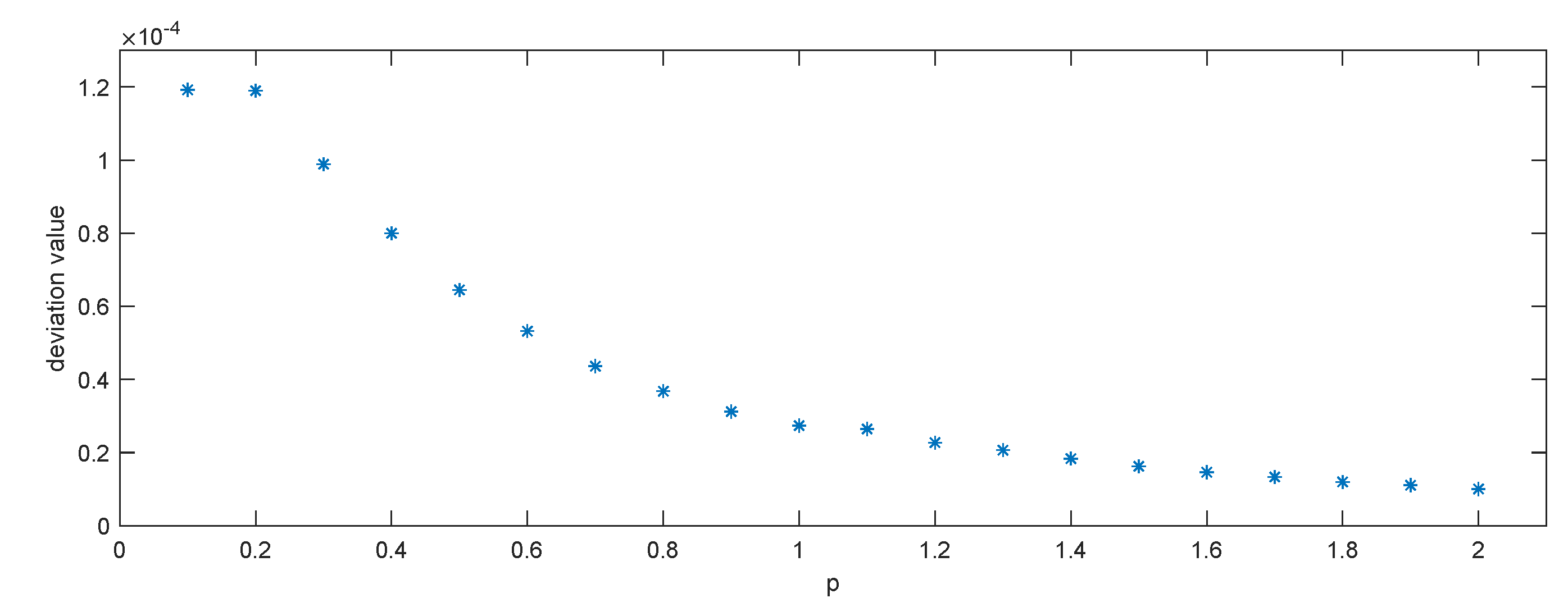
With the change in the method of numerical integration, we obtained another series of price f ˜ . From Table 2, we can intuitively observe that the prices of option changed little, and some were the same in both tables. There existed a round-off error among computer calculations, the methodical errors of the two numerical methods were small enough to be ignored. Calculating f ˜ f then generated Figure 1.
As is shown in Figure 1, most of the deviation values of prices were smaller than 10 4 and becoming smaller. The values of f in the table were saved as four-digit decimals, so the change in the numerical integration formula made little difference.
Remark 3.
Though the compound Simpson formula has better algebraic precision, the application of the compound trapezoid formula is more appropriate because of the shorter computing time and it being easy for code writing.
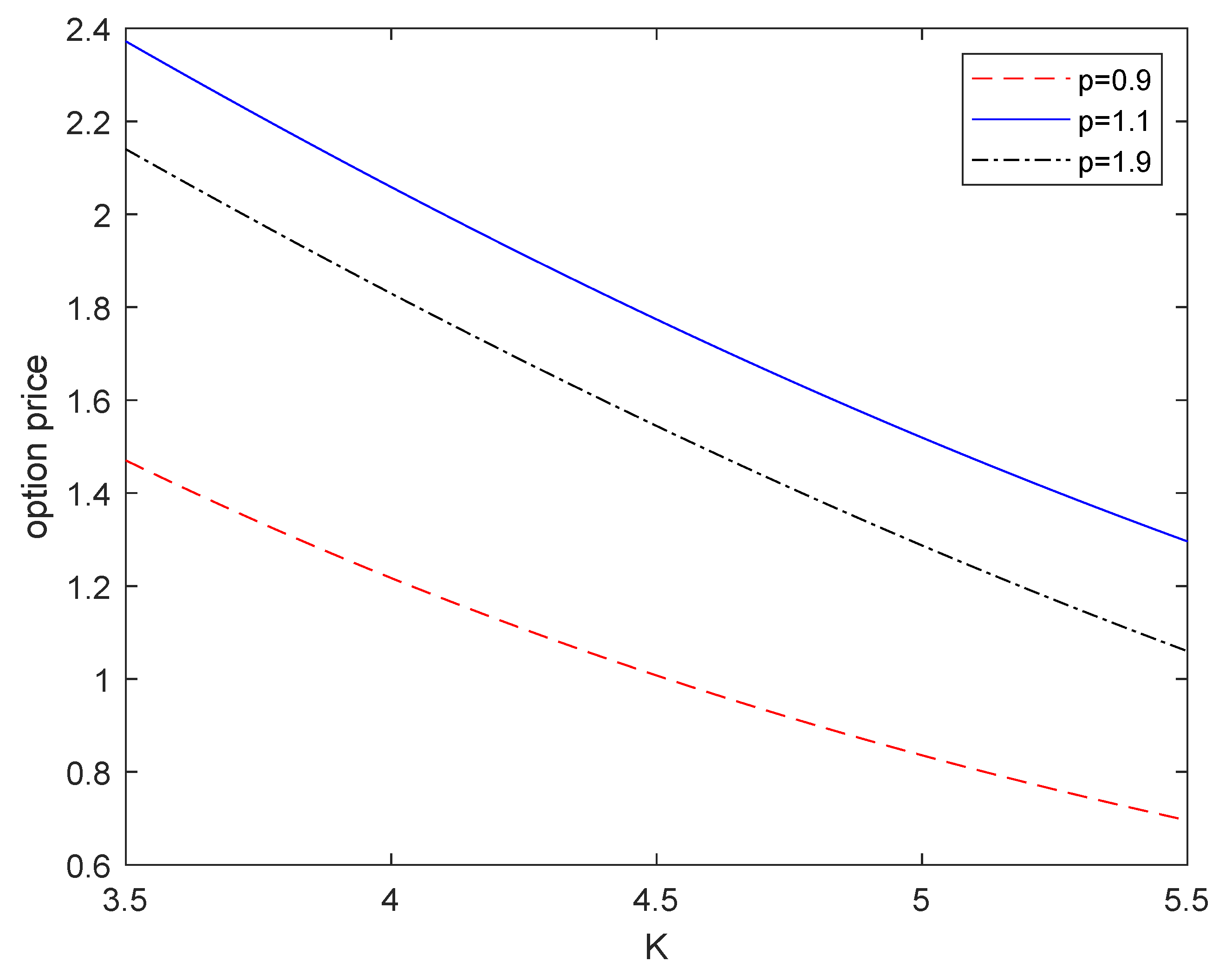
Now, we discuss the European currency option price with a constant p and different K, considering that K in [ 3.5 , 5.5 ] and p = 0.9 , 1.1 , 1.9 . With the comparison of the two numerical methods above, we used the compound trapezoid formula to calculate numerical integration and obtain f. Then, we could generate Figure 2.
As is illustrated in Figure 2, for different p, price f was a decreasing function of K, and its decrease was nonlinear. Such a conclusion could also be obtained by observing the structure of Function (17). While K increased, the values of Z T K + and 1 K K Z T Z T + decreased or were equal to 0.
Remark 4.
The price of European currency option f in this paper was a decreasing function of K, while other parameters were constant, which is similar to the result in Liu et al. [28] for UDEs.
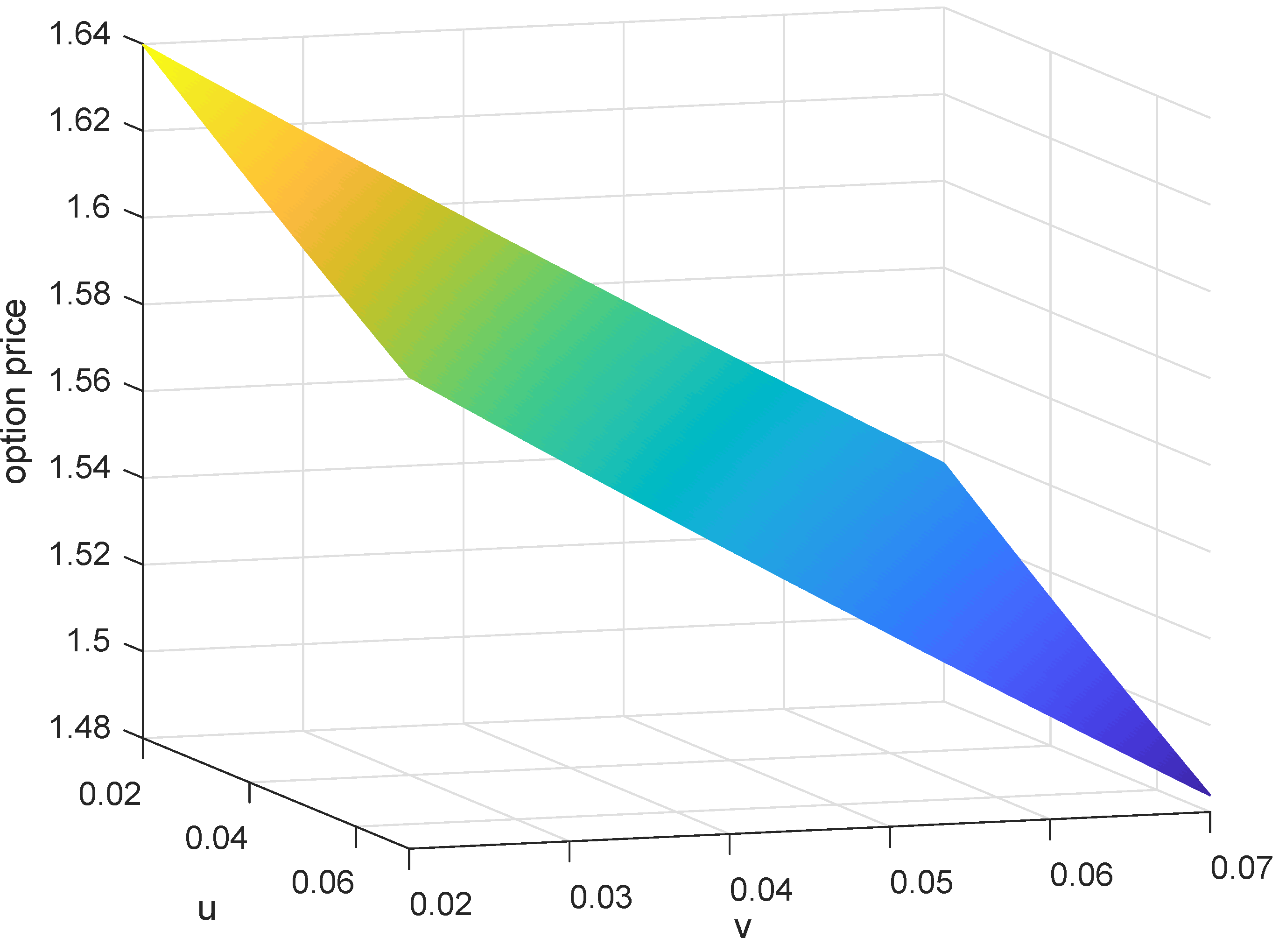
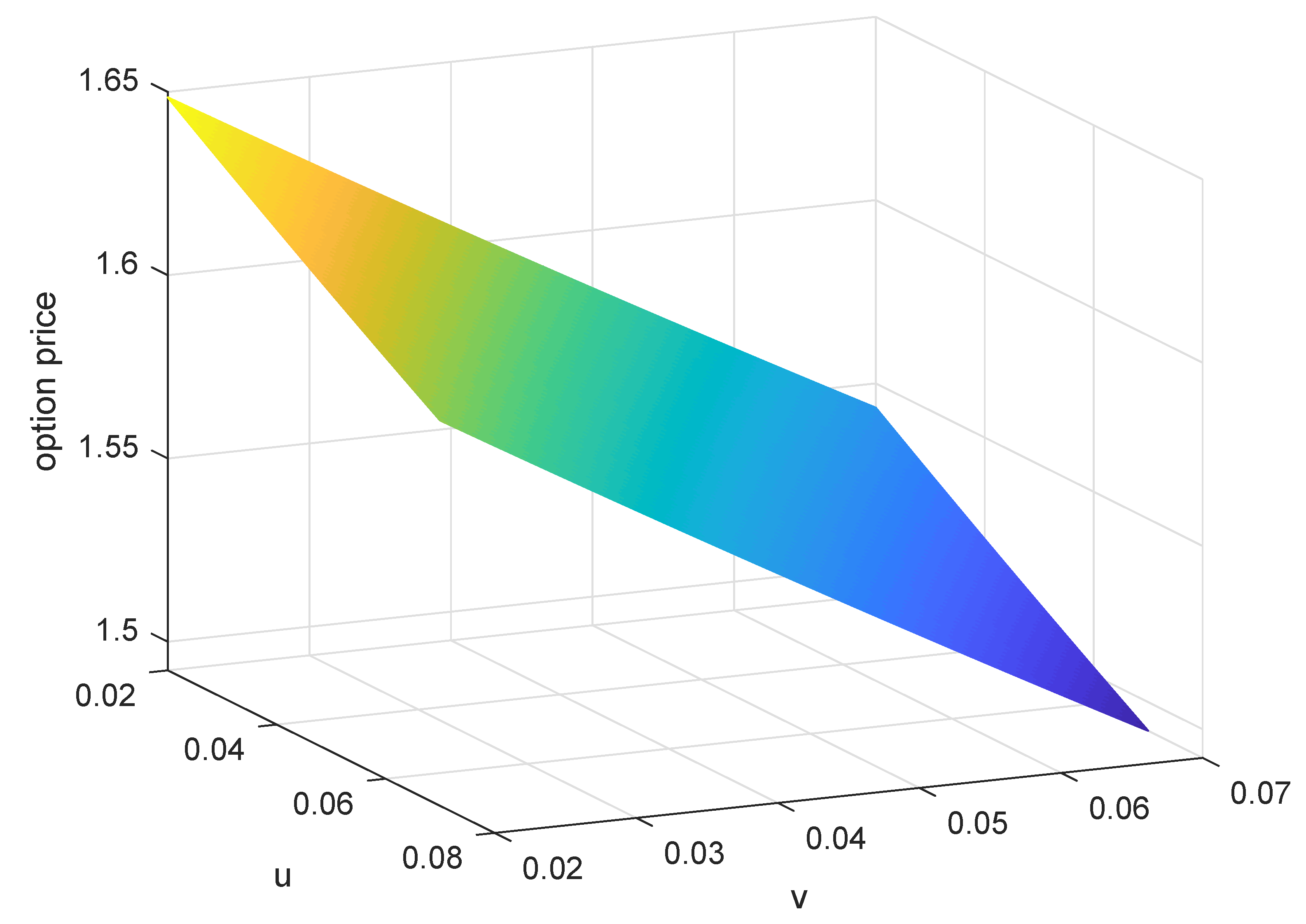
Now, we discuss the European currency option price with p = 1.9 and K = 4.5 , considering the variation of the price while u and v changed in [ 0.02 , 0.07 ] . With the comparison of the two numerical methods above, we used the compound trapezoid formula to calculate numerical integration and obtain f. Then, we could generate Figure 3.
As is shown in Figure 3, price f was a decreasing function of both u and v. In Function (17), taking derivatives in u and v, the decrease was nonlinear. In addition, as u and v increased simultaneously, the value of price f decreased.
Remark 5.
The price of European currency option f in this paper was a decreasing function of both u and v, while other parameters were constant, which is similar to the result in Liu et al. [28] for UDEs.

5.2. American Currency Option Pricing

Example 2.
We assumed that uncertain fractional currency Model (13) had u = 6 % , v = 3 % , e = 0.05 , σ = 0.3 , and the initial exchange rate Z 0 = 4.2 , p ( 0 , 2 ) , and considered the American currency option with expiration date T = 2 and striking price K = 4.5 .
In this numerical example, similar to the previous example, the two currencies were RMB and SGD, and the initial exchange rate Z 0 was changed a little. These two currencies and the financial markets in both countries were considered to be stable enough, so the parameters in the example were reasonable. As in the previous example, z 1 = 0.7861 represents the derivative of the exchange rate at t = 0 .
Due to the particularity of the American currency option whose price is influenced by the maximal Z s , s 0 , T , we viewed Z s as a discrete instead of a continuous case. It could also be reasonable to set the interval to be small enough and reduce the computing time. To solve the problem in this example, we divided the whole time T into 100 equal intervals. Hence, our work turned to calculating the maximum of these 100 values to obtain American currency option price f.
Similar to the previous example, we used the compound trapezoid and Simpson formulas whose interval values were both 0.001 to compute the integral of α over 0 , 1 . We first used the compound trapezoid formula to calculate American currency option price f; results are shown in Table 3.
As is shown in Table 3, the price of the American currency option increased with the increase in p in 0 , 0.8 , and decreased with the increase in p in 0.8 , 1 and 1.1 , 2 . The price jumped when p changed from 1.0 to 1.1 because of the initial value of Z 0 , similar to the price function of the European currency option. Such a jump is similar to that in the results obtained by Lu [26]. Obviously, different initial values may cause different values of price f.
Meanwhile, the value of prices were the same as that of the European currency option when p 1 . That is to say, with the setting of u = 6 % , v = 3 % , e = 0.05 , σ = 0.3 , p 1 , and initial exchange rate Z 0 = 4.2 , American currency option price f was an increasing function of time s.
Now, we change the method of numerical integration. With the use of the compound Simpson formula, we obtained the American currency option price f in Table 4.
With the change in the method of numerical integration, we obtain another series of price f ˜ . From Table 4, we can intuitively observe that the prices of option changed little, and some were the same in the two tables. Similar to the previous part, we calculated f ˜ f and generated Figure 4.
As is shown in Figure 4, most of the deviation values of prices were smaller than 10 4 and becoming smaller. For the same reason, we still chose the compound trapezoid formula instead of the compound Simpson formula.
Remark 6.
Similar to Remark 3, though the compound Simpson formula has better algebraic precision, the application of the compound trapezoid formula is more appropriate because of the shorter computing time and it being easy for code writing.
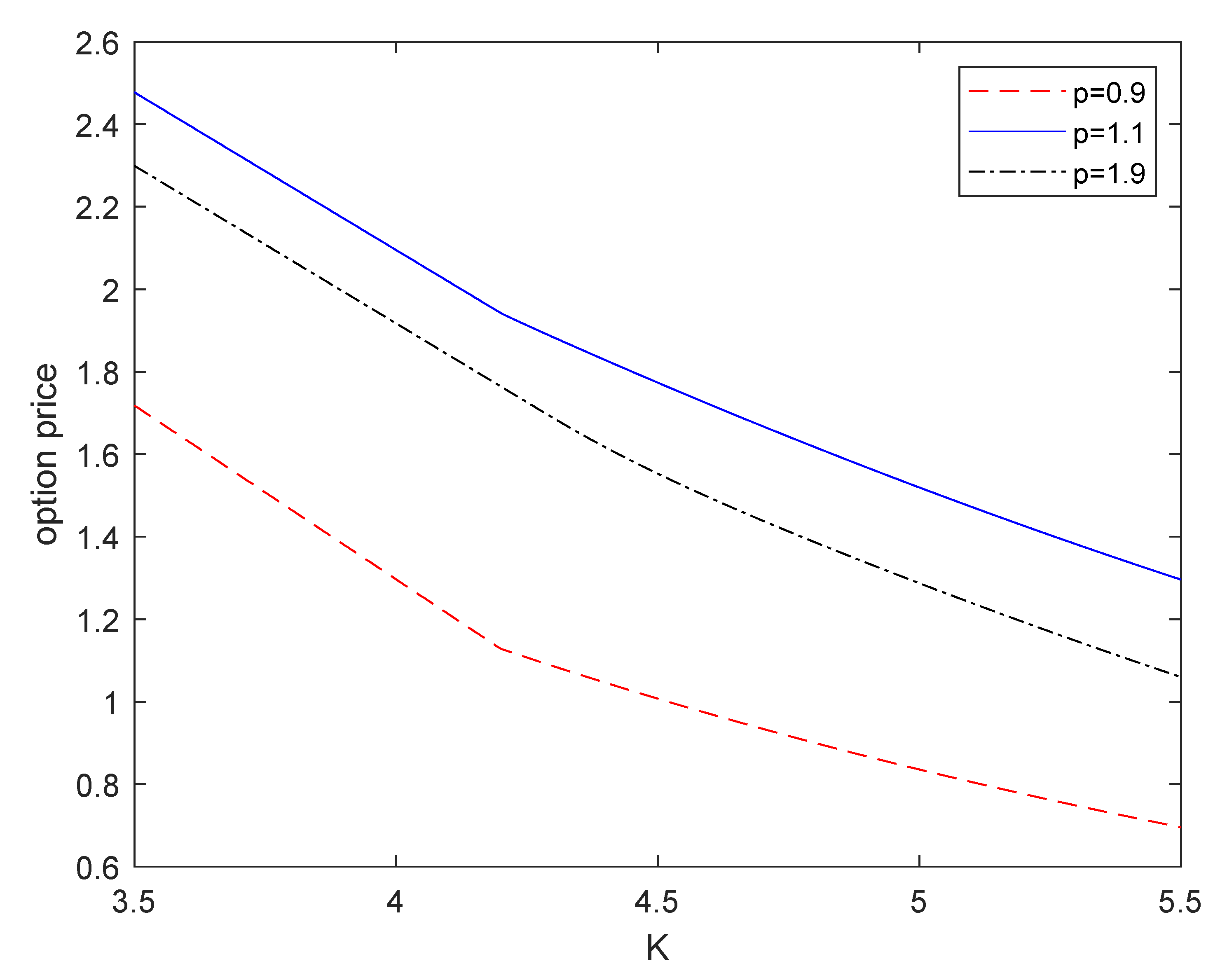
Now, we discuss the American currency option price with a constant p and different K, considering that K was [ 3.5 , 5.5 ] and p = 0.9 , 1.1 , 1.9 . With the comparison of two numerical methods above, we used the compound trapezoid formula to calculate the numerical integration and obtain f. Then, we could generate Figure 5.
As is illustrated in Figure 5, for the different p, price f was a decreasing function of K, and its decrease was nonlinear. Such a conclusion could also be obtained by observing the structure of Function (20). While K increased, the values of sup 0 s T exp ( u s ) ( Z s K ) + and sup 0 s T Z 0 exp ( v s ) ( 1 K / Z s ) + decreased or were equal to 0.
Remark 7.
Similar to Remark 4, the price of American currency option f in this paper was a decreasing function of K, while other parameters were constant, which is similar to the result in Liu et al. [28] for UDEs.
Now, we discuss the American currency option price with p = 1.9 and K = 4.5 , considering variation in the price while u and v were changed in [ 0.02 , 0.07 ] . With the comparison of the two numerical methods above, we used the compound trapezoid formula to calculate the numerical integration and obtain f. Then, we could generate Figure 6.
As is shown in Figure 6, price f was a decreasing function of both u and v. In Function (20), taking derivatives in u and v, the decrease was nonlinear. In addition, as u and v increased simultaneously, the value of price f decreased.
Remark 8.
The price of American currency option f in this paper was a decreasing function of both u and v, while other parameters were constant, which is similar to the result in Liu et al. [28] for UDEs.

6. Conclusions

In this paper, two option pricing formulas were given that use the Mittag-Leffler function to solve fractional differential equations in the Caputo sense. Moreover, the exchange rate of two currencies Z t is driven by geometric Liu process. An uncertain fractional currency model was presented, and the option pricing formulas were proposed. Both option prices (European and American currency options) of that model had the same monotonicity as that in previous works that price f (for both the European and American currency options) was a decreasing function of exercise price K and interest rates u and v. Lastly, two given numerical examples illustrated the prices of the currency options under different p ( p 0 , 2 ) . Future work could modify the price function with the parameters of log-drift e and log-diffusion σ , and examine the relationship between the price jump and its decrease while some parameters are constant. Moreover, the interpretations for the decrease in mathematical and practical meaning in real life can be another future direction.

Author Contributions

Conceptualization, T.J.; Data curation, Q.L.; Formal analysis, Q.L.; Funding acquisition, M.Z. and D.J.; Investigation, F.L.; and D.J.; Methodology, T.J.; Project administration, M.Z.; Resources, T.J., M.Z. and D.J.; Software, Q.L. and C.T.; Supervision, T.J.; Validation, C.T.; Writing—original draft, Q.L.; Writing—review & editing, F.L. All authors have read and agreed to the published version of the manuscript.

Funding

This research was funded by the National Natural Science Foundation of China grant number no.12071219 and the Natural Science Foundation of Jiangsu Province grant number no. BK20210605. This work is also supported by the Academic Program Development of Jiangsu Higher Education Institutions (PAPD), the General Research Projects of Philosophy and Social Sciences in Colleges and Universities (2022SJYB0140), the Jiangsu Province Student Innovation Training Program (202110298040Z and 202210298050Z), and Postgraduate Research & Practice Innovation Program of Jiangsu Province (SJCX22_0311).

Institutional Review Board Statement

Not applicable.

Informed Consent Statement

Not applicable.

Data Availability Statement

Data sharing is not applicable to this article as no datasets were generated or analyzed during the current study.

Conflicts of Interest

The authors declare no conflict of interest.

References

  1. Soleymani, F.; Itkin, A. Pricing foreign exchange options under stochastic volatility and interest rates using an RBF–FD method. J. Comput. Sci. 2019, 37, 101028. [Google Scholar] [CrossRef]
  2. Alvise, D.; Alessandro, G.; Martino, G. Smiles all around: FX joint calibration in a multi-Heston model. J. Bank. Financ. 2013, 37, 3799–3818. [Google Scholar] [CrossRef]
  3. Tversky, K. Prospect Theory: An Analysis of Decision under Risk. Econometrica 1979, 47, 163–291. [Google Scholar]
  4. Liu, B. Uncertainty Theory; Springer: Berlin/Heidelberg, Germany, 2007. [Google Scholar]
  5. Liu, B. Uncertainty Theory: A Branch of Mathmatics for Modeling Human Uncertainty; Springer: Berlin/Heidelberg, Germany, 2011. [Google Scholar]
  6. Liu, B. Some research problems in uncertainty theory. J. Uncertain Syst. 2009, 3, 3–10. [Google Scholar]
  7. Liu, B. Fuzzy Process, Hybrid Process and Uncertain Process. J. Uncertain Syst. 2008, 2, 3–16. [Google Scholar]
  8. Chen, X.; Liu, B. Existence and uniqueness theorem for uncertain differential equations. Fuzzy Optim. Decis. Mak. 2010, 9, 69–81. [Google Scholar] [CrossRef]
  9. Gao, Y. Existence and Uniqueness Theorem on Uncertain Differential Equations with Local Lipschitz Condition. J. Uncertain Syst. 2012, 6, 223–232. [Google Scholar]
  10. Yao, K.; Chen, X. A numerical method for solving uncertain differential equations. J. Intell. Fuzzy Syst. 2013, 25, 825–832. [Google Scholar] [CrossRef]
  11. Chen, X. American option pricing formula for uncertain financial market. In Proceedings of the First International Conference on Uncertainty Theory, Berlin, Germany, 22–23 November 2010. [Google Scholar]
  12. Peng, J.; Yao, K. A new option pricing model for stocks in uncertainty markets. Int. J. Oper. Res. 2010, 7, 213–224. [Google Scholar]
  13. Gao, R.; Liu, K.; Li, Z.; Lv, R. American Barrier Option Pricing Formulas for Stock Model in Uncertain Environment. IEEE Access 2019, 7, 97846–97856. [Google Scholar] [CrossRef]
  14. Chang, J.; Sun, L.; Zhang, B.; Peng, J. Multi-period portfolio selection with mental accounts and realistic constraints based on uncertainty theory. J. Comput. Appl. Math. 2020, 377, 112892. [Google Scholar] [CrossRef]
  15. Chen, X.; Gao, J. Uncertain term structure model of interest rate. Soft Comput. 2013, 17, 597–604. [Google Scholar] [CrossRef]
  16. Liu, B. Extreme value theorems of uncertain process with application to insurance risk models. Soft Comput. 2013, 17, 549–556. [Google Scholar] [CrossRef]
  17. Lakshmikantham, V.; Vatsala, A. Theory of fractional differential equations. Nonlinear Anal. 2008, 69, 2677–2782. [Google Scholar] [CrossRef]
  18. Lakshmikantham, V.; Devi, J. Theory of fractional differential equations in Banach space. Nonlinear Anal. 2008, 1, 38–45. [Google Scholar]
  19. Belmekki, M.; Nieto, J.; Rodríguez-López, R. Existence of Periodic Solution for a Nonlinear Fractional Differential Equation. Bound. Value Probl. 2009, 2009, 324561. [Google Scholar] [CrossRef]
  20. Kosmatov, N. Integral equations and initial value problems for nonlinear differential equations of fractional order. Nonlinear Anal. Theory Methods Appl. 2019, 70, 2521–2529. [Google Scholar] [CrossRef]
  21. Zhang, S. Monotone iterative method for initial value problem involving Riemann–Liouville fractional derivatives. Nonlinear Anal. Theory Methods Appl. 2009, 71, 2087–2093. [Google Scholar] [CrossRef]
  22. Zhu, Y. Uncertain fractional differential equations and an interest rate model. Math. Methods Appl. Sci. 2015, 38, 3359–3368. [Google Scholar] [CrossRef]
  23. Zhu, Y. Existence and uniqueness of the solution to uncertain fractional differential equation. Uncertain. Anal. Appl. 2015, 3, 5. [Google Scholar] [CrossRef]
  24. Jin, T.; Sun, Y.; Zhu, Y. Extreme values for solution to uncertain fractional differential equation and application to American option pricing model. Phys. A Stat. Mech. Its Appl. 2019, 534, 122357. [Google Scholar] [CrossRef]
  25. Lu, Z.; Zhu, Y.; Li, B. Critical value-based Asian option pricing model for uncertain financial markets. Phys. A Stat. Mech. Its Appl. 2019, 525, 694–703. [Google Scholar] [CrossRef]
  26. Lu, Z.; Yan, H.; Zhu, Y. European option pricing model based on uncertain frational differential equation. Fuzzy Optim. Decis. Mak. 2019, 18, 199–217. [Google Scholar] [CrossRef]
  27. Lu, Z.; Zhu, Y. Numerical approach for solution to an uncertain fractional differential equation. Appl. Math. Comput. 2019, 343, 137–148. [Google Scholar] [CrossRef]
  28. Liu, Y.; Chen, X.; Ralescu, D. Uncertain Currency Model and Currency Option Pricing. Int. J. Intell. Syst. 2015, 30, 40–51. [Google Scholar] [CrossRef]
  29. Diethelm, K.; Ford, N.; Freed, A. A Predictor-Corrector Approach for the Numerical Solution of Fractional Differential Equations. Nonlinear Dyn. 2002, 29, 3–22. [Google Scholar] [CrossRef]
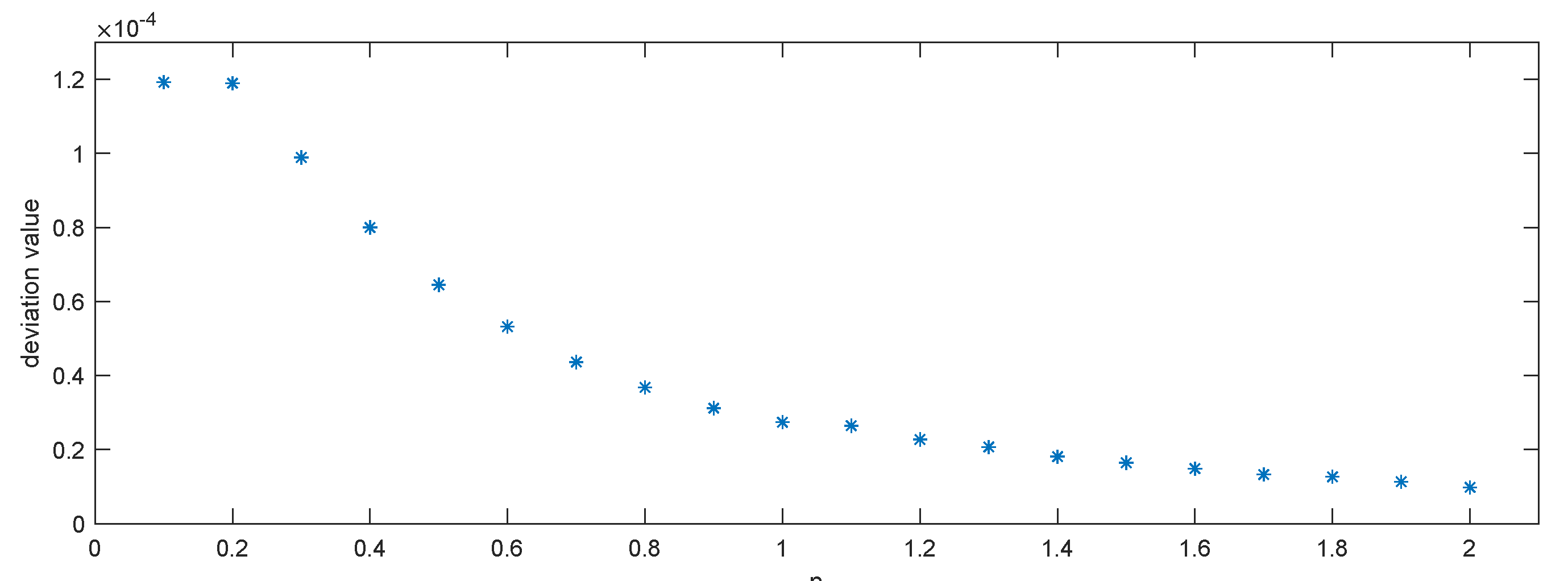
Figure 1. The deviation value of prices f ˜ f between two formulas with different p.
Fractalfract 06 00407 g001
Figure 2. The price of the option with different K in [ 3.5 , 5.5 ] while p is constant.
Fractalfract 06 00407 g002
Figure 3. The price of the option with different u , v in [ 3.5 , 5.5 ] while p = 1.9 , K = 4.5 .
Fractalfract 06 00407 g003
Figure 4. The deviation value of prices f ˜ f between two formulas with different p.
Fractalfract 06 00407 g004
Figure 5. Price of the option with different K in [ 3.5 , 5.5 ] while p is constant.
Fractalfract 06 00407 g005
Figure 6. The price of the option with different u , v in [ 3.5 , 5.5 ] while p = 1.9 , K = 4.5 .
Fractalfract 06 00407 g006
Table 1. Price of the European option with different p (compound Trapezoid formula).
p0.10.20.30.40.50.60.70.80.91.0
f0.70900.81470.89000.94200.97650.99771.00861.01131.00750.9986
p1.11.21.31.41.51.61.71.81.92.0
f1.77371.74891.72231.69431.66541.63571.60551.57501.54441.5138
Table 2. Price of the European option with different p (compound Simpson formula).
p0.10.20.30.40.50.60.70.80.91.0
f ˜ 0.70890.81460.88990.94190.97650.99771.00851.01121.00750.9985
p1.11.21.31.41.51.61.71.81.92.0
f ˜ 1.77361.74881.72221.69431.66531.63571.60551.57501.54441.5138
Table 3. Price of the American option with different p (compound trapezoid formula).
p0.10.20.30.40.50.60.70.80.91.0
f0.70900.81470.89000.94200.97650.99771.00861.01131.00750.9986
p1.11.21.31.41.51.61.71.81.92.0
f1.77371.74891.72231.69471.66651.63801.60941.58101.55291.5253
Table 4. Price of the American option with different p (compound Simpson formula).
p0.10.20.30.40.50.60.70.80.91.0
f0.70890.81460.88990.94190.97650.99771.00851.01121.00750.9985
p1.11.21.31.41.51.61.71.81.92.0
f1.77361.74881.72231.69471.66651.63791.60941.58101.55291.5253
Publisher’s Note: MDPI stays neutral with regard to jurisdictional claims in published maps and institutional affiliations.