Some Properties of Fractional Cumulative Residual Entropy and Fractional Conditional Cumulative Residual Entropy

Abstract

Fractional cumulative residual entropy is a powerful tool for the analysis of complex systems. In this paper, we first provide some properties of fractional cumulative residual entropy (FCRE). Secondly, we generate cumulative residual entropy (CRE) to the case of conditional entropy, named fractional conditional cumulative residual entropy (FCCRE), and introduce some properties. Then, we verify the validity of these properties with randomly generated sequences that follow different distributions. Moreover, we give the definition of empirical fractional conditional accumulative residual entropy and prove that it can be used to approximate FCCRE. Finally, the empirical analysis of the aero-engine gas path data is carried out. The results show that FCRE and FCCRE can effectively capture complex information in the gas path system.

1. Introduction

In 1948, C.E. Shannon gave the concept of information entropy in a discrete distribution based on thermodynamic entropy [1,2].

$$H(U)=-{\displaystyle \sum _{j=1}^n{p}_j}\log p_j,$$

(1)

where $p_j$ are the probability density function of $U$.

When $U$ is a non-negative continuous random variable with density $f(u)$, Shannon entropy for the continuous case is given below.

Shannon entropy has made great achievements in many fields, not only in

$$H(u)=-{\displaystyle {\int }_0^{\infty }f(u)\log f(u)du}.$$

(2)

information theory but also in financial analysis [3], communications [4], and statistics [5]. Therefore, a mass of innovative scientific research, based on the Shannon entropy, such as transfer entropy [6], Rényi entropy [7], etc., have been raised.

Despite its enormous success, the following cases show that this method may be inappropriate for some situations. It is only defined for distributions with densities. For example, there is no definition of entropy for a mixture of densities with different distributions. These things considered, in general, the differential entropy of continuous variables cannot be approximated by the entropy of empirical distributions.

In order to better extend Shannon entropy to random variables with continuous distribution, Murali Rao et al. put forward the concept of cumulative residual entropy (CRE) [8]:

$$\epsilon ({\overline{F}}_U)=-{\displaystyle {\int }_0^{\infty }\overline{F}(u)\log \overline{F}(u)du},$$

(3)

through the survival function $\overline{F}\left(u\right)=1-F(u)$ of $U$, where $F(u)$ is the cumulative distribution function of $U$. When $U=\left(U_1,U_2,\dots ,U_N\right)$ is a random vector, the cumulative residual entropy is also defined as $\epsilon ({\overline{F}}_U)=-{\displaystyle {\int }_0^{\infty }\overline{F}(u)\log \overline{F}(u)du}$ [8]. Compared with the density function in Shannon’s definition, the distribution function is more regular. It has coincident definitions in continuous and discrete cases and is easily computed from sample data. Based on the superior properties of CRE, many new concepts of entropy have been proposed [9,10,11,12,13,14,15].

In practical applications, we might need to explore the uncertainty between two messages [16]. In 2004, Murali Rao et al. also defined conditional cumulative residual entropy (CCRE) [8]:

$$\epsilon (U\left|\eta \right.)=-{\displaystyle {\int }_{R_{+}^N}p(\left|U\right|>u\left|\eta \right.)}\log p(\left|U\right|>u\left|\eta \right.)du,$$

(4)

where $\eta$ is an $\sigma$-field. Conditional entropy plays an important role in information measurement not only in mathematics and communication, but also in many fields such as physics, biology, and computer applications [17,18,19,20].

To describe phenomena outside the scope of Boltzmann–Gibbs formalism, M. Rao et al. proposed entropy based on the fractional calculus [21].

$$s_q(p)={\displaystyle \sum _j{p}_j{(-\log p_j)}^q}, 0<q\le 1.$$

(5)

Obviously, Shannon entropy is the case of $q=1$. Fractional entropy has many special properties, such as positive, concave, and non-additive. The study in Ref. [22] shows it satisfies Lesche and thermodynamic stability and has higher sensitivity to signal evolution, which is more beneficial for describing the dynamics of complex systems. Thus, FCRE has been extended to diverse general cases [23,24,25,26].

Recently, inspired by CRE and fractional entropy, H. Xiong et al. introduced a new expression of entropy, named fractional cumulative residual entropy (FCRE) [27].

$${\epsilon }_q({\overline{F}}_U)={\displaystyle {\int }_0^{\infty }\overline{F}(u){\left[-\log \overline{F}(u)\right]}^{q}du}, 0<q\le 1.$$

(6)

In particular, fractional CRE degenerates into CRE when the parameter $q$ is equal to 1. In addition, it is evident that ${\epsilon }_0\left({\overline{F}}_U\right)=E\left(U\right)$. When $U=\left(U_1,U_2,\dots ,U_N\right)$ is a random vector, its fractional cumulative residual entropy can still be obtained by Equation (6).

In this paper, we first produced some new results on fractional cumulative residual entropy. Many research works on entropy manifest that conditional entropy provides a method to describe the interaction between two kinds of information [17,18,19,20]. Hence, inspired by the research mentioned above [8,21,27], we propose the fractional-order calculation for CCRE to obtain an improved concept of entropy, named fractional-order conditional cumulative residual entropy (FCCRE), and discuss the properties of conditional fractional CRE.

The remaining part of the paper is organized as follows: Section 2 presents some properties of fractional cumulative residual entropy and gives some simulations to show the reliability of FCRE. In Section 3, we define fractional conditional CRE and introduce some properties of fractional conditional cumulative entropy. Then, the sample data are used to verify the reliability of these properties. Section 4 presents empirical FCCRE and discusses its properties. In Section 5, we discuss the application of the FCRE and FCCRE methods in the aero-engine gas path system. Finally, Section 6 draws some conclusions.

2. Some Properties of FCRE

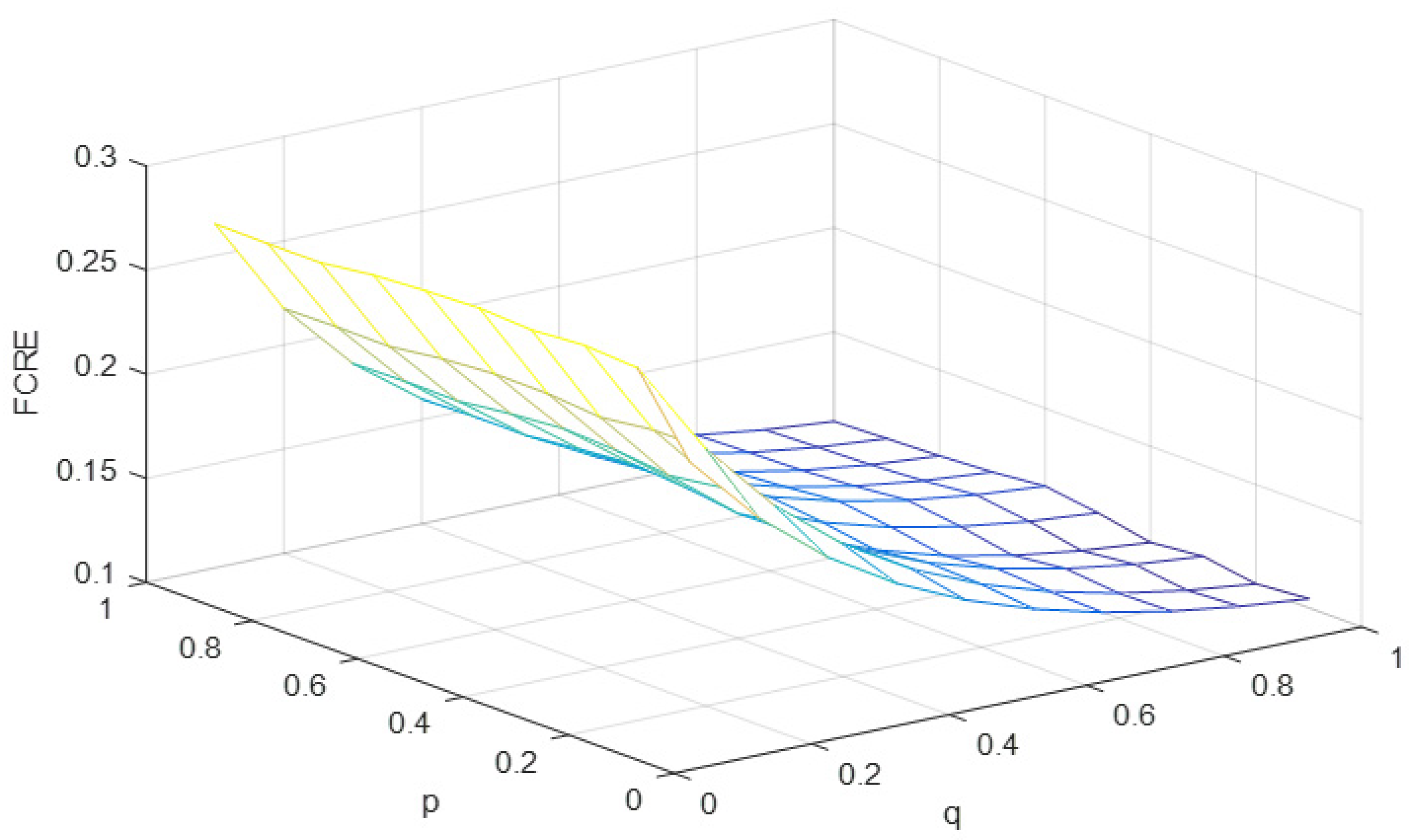
In this section, some properties of FCRE are given. Before introducing these properties, we display the relationship among FCRE, the probabilities $P$, and the fractional order $q$, as seen in Figure 1, where $P$ is the probability calculated by the residual distribution function. In the following examples, we use the sample data generated by one of the typical distribution functions to display the change in FCRE or FCCRE with different values $q$ on $[0, 1]$, and other distribution functions can also achieve the experimental effect.

Figure 1. The relationship among fractional cumulative residual entropy, fractional order $q$, and probability $P$ for typical examples of the uniform distribution on $[0, 1]$.

Proposition 1.

Let$U$be a random vector, then

$${\epsilon }_q({\stackrel{-}{F}}_U)\ge 0,$$

the identity holds when$P\left(\left|U\right|=A\right)=1$, which means the probability of${\left|U\right|}_j=A_j$is 1, where$A_j$is the$jth$component of the vector$A=\{A_1,A_2,\cdots ,A_n\}$.

Proof of Proposition 1.

If the equation holds, consider

$$u{(-\log u)}^q=0,$$

for all $0<q\le 1$, is established if and only if $u=0$ or $u=1$.

So, ${\epsilon }_q({\stackrel{-}{F}}_U)=0$ means $P\left(\left|U\right|>A\right)=0$ or $P\left(\left|U\right|>A\right)=1$ for all $A$.

When $P\left(\left|U\right|>A\right)=0$, then $P\left(\left|U\right|=0\right)=1$.

Consider $P\left(\left|U\right|>A\right)=1$ holds for all $A$, and $\alpha =\underset{A\in \phi }{\max }A$, then $\alpha$ satisfies

$$P\left(\left|U\right|=\alpha \right)=1,$$

where $\phi =\left\{A|P\left(\left|U\right|>A\right)=1\right\}$. The proposition is proved. □

Example 1.

Assuming that$U$is an arbitrary constant column denoted by ‘constant sequence’, and the random sequence$V$is formed out of uniform distribution on$[0, 1]$denoted by ‘uniform distribution’. Then, the condition of Proposition 1 is satisfied. The result is shown in Figure 2.

Figure 2. The fractional cumulative residual entropy of constant sequence and uniform distribution on $[0, 1]$.

Proposition 2.

Let$U$and$V$be two independent non-negative random variables,

$$\max \left({\epsilon }_q(U),{\epsilon }_q(V)\right)\le {\epsilon }_q(U+V).$$

(7)

Proof of Proposition 2.

Since $U$ and $V$ are independent, then

$$P\left[U+V>t\right]={\displaystyle \int d{F}_V\left(c\right)P\left[U>t-c\right]},$$

where $F_V$ represents the cumulative distribution function of $V$.

Since ${\overline{F}}_U\le {\left[{\overline{F}}_U\right]}^q$ for all $u\in U,u>0$ and $0<q\le 1$ where ${\stackrel{-}{F}}_U$ means the survival function of $U$.

$$-{\epsilon }_q\left(U+V\right)\le {\epsilon }_q(U+V)={\displaystyle {\int }_0^{\infty }{\stackrel{-}{F}}_{U+V}{\left[-\log {\stackrel{-}{F}}_{U+V}\right]}^{q}du}\le {\displaystyle {\int }_0^{\infty }{\left[-{\stackrel{-}{F}}_{U+V}\log {\stackrel{-}{F}}_{U+V}\right]}^{q}du},$$

where ${\overline{F}}_{U+V}$ is the survival function of $U+V$.

According to Jensen’s inequality,

$${\left[P\left[U+V>t\right]\left|\log P\left[U+V>t\right]\right|\right]}^q\le {\displaystyle \int d{F}_V\left(c\right){\left[P\left[U>t-c\right]\left|\log P\left[U>t-c\right]\right|\right]}^q}.$$

Integrating both sides of the above formula from 0 to $\infty$,

$$\begin{array}{c}-{\epsilon }_q\left(U+V\right)\le {\displaystyle \int d{F}_V\left(c\right){\displaystyle {\int }_0^{\infty }{\left[P\left[U>t-c\right]\left|\log P\left[U>t-c\right]\right|\right]}^q}}dt\hfill \\ ={\displaystyle \int d{F}_V\left(c\right){\displaystyle {\int }_c^{\infty }{\left[P\left[U>t-c\right]\left|\log P\left[U>t-c\right]\right|\right]}^q}}dt\hfill \\ =-{\displaystyle \int d{F}_{V(c)}}{\epsilon }_q({\stackrel{-}{F}}_U)\hfill \\ =-{\epsilon }_q(U).\hfill \end{array}$$

When $t\le c,P\left[U>t-c\right]=1$. The proposition is proved. □

Example 2.

Suppose$U$follows a uniform distribution on$[0, 1]$, $V$follows an exponential distribution with $\lambda =0.5$. Then, the distribution function of$W=U+V$is$F\left(W\right)=\frac{e^{\lambda }\left(e^b-e^a\right)}{\lambda (a-b)}\left(e^{-\lambda W}-1\right)$. The simulated result is shown in Figure 3. It is evident that the FCRE of the sum of two random variables is greater than that of either random variable, which is in accordance with Proposition 2.

Figure 3. The fractional cumulative residual entropy of the uniform distribution, exponential distribution, and the distribution $F\left(W\right)$.

Weak convergence is a significant property in statistics [28]. Combining the theorem 1 in Ref. [25], there is the following proposition.

Proposition 3.

Given random vector$U_n$that converges to the random vector $U$in distribution, then for any bounded continuous functions$\varphi$on$R_N$,

$$\underset{n\to \infty }{\lim }E\left[\varphi (U_n)\right]=E\left[\varphi (U)\right].$$

(8)

For some$p>N$, if all the $U_n$are bounded in$L^P$, we have

$${\epsilon }_q(U_n)\stackrel{a.s.}{\to }{\epsilon }_q(U),n\to \infty .$$

(9)

Proof of Proposition 3.

Let $U_n$ converge to the random vector $U$ in distribution [29]; it is known that

$$\underset{n\to \infty }{\lim }P\left[\left|U_n\right|>u\right]=P\left[\left|U\right|>u\right],$$

for all $u$ on $R_N^{+}$.

Then,

$$\underset{n\to \infty }{\lim }P\left[\left|U_n\right|>u\right]\log P\left[\left|U_n\right|>u\right]=P\left[\left|U\right|>u\right]\log P\left[\left|U\right|>u\right].$$

From Theorem 1 in Ref. [8], we know

$${\left[P\left[\left|U_n\right|>u\right]\left|\log P\left[\left|U_n\right|>u\right]\right|\right]}^q\le {\left(\frac{e^{-1}}{1-\alpha }\right)}^q{\left[{\displaystyle \prod _{j=1}^{N}P{\left[\left|U_{n_j}\right|>u_j\right]}^{\raisebox{1ex}{$\alpha $}\!\left/ \!\raisebox{-1ex}{$N$}\right.}}\right]}^q,$$

for each n and $j$.

Therefore,

$$\begin{gathered} {\displaystyle {\int }_0^{\infty }P{\left[\left|U_{n_i}\right|>u_i\right]}^{\raisebox{1ex}{$q\alpha $}\!\left/ \!\raisebox{-1ex}{$N$}\right.}du}={\displaystyle {\int }_0^{1}P{\left[\left|U_{n_j}\right|>u_j\right]}^{\raisebox{1ex}{$q\alpha $}\!\left/ \!\raisebox{-1ex}{$N$}\right.}du}+{\displaystyle {\int }_1^{\infty }P{\left[\left|U_{n_j}\right|>u_j\right]}^{\raisebox{1ex}{$q\alpha $}\!\left/ \!\raisebox{-1ex}{$N$}\right.}du} \\ \le 1+{\displaystyle {\int }_1^{\infty }{\left\{\frac{1}{u_j{}^p}E\left[{\left|U_{n_j}\right|}^p\right]\right\}}^{\raisebox{1ex}{$q\alpha $}\!\left/ \!\raisebox{-1ex}{$N$}\right.}du}, \end{gathered}$$

(10)

where $\frac{pq\alpha }{N}>1$. The proposition is proved. □

Proposition 4.

For a non-negative random variable$U$and$0<q\le 1$, it holds that${\epsilon }_q\left(U\right)\le {\left[\epsilon \left(U\left(\lambda \right)\right)\right]}^q$, where$U\left(\lambda \right)$is the exponentially distributed random variable with mean$\lambda =E\left(U^2\right)/2E\left(U\right)$.

Proof of Proposition 4.

Since $\overline{F}(u)\le {\left[\overline{F}(u)\right]}^q$ for $u>0$ and $0<q\le 1$,

$$\begin{gathered} {\epsilon }_q(U)={\displaystyle {\int }_0^{\infty }\overline{F}(U){\left[-\log \overline{F}(U)\right]}^{q}du \\ }\le {\displaystyle {\int }_0^{\infty }{\left[-\overline{F}(U)\log \overline{F}(U)\right]}^{q}du}\le {\left[{\displaystyle {\int }_0^{\infty }-\overline{F}(U)\log \overline{F}(U)du}\right]}^q={\left[\epsilon (U)\right]}^q, \end{gathered}$$

(11)

where the last inequality is attained from Jensen’s inequality. The equality holds at $q=1$.

Then, by log-sum inequality

$${\displaystyle {\int }_0^{\infty }p\left(U>t\right)\log \left(e^{t/\lambda }p\left(U>t\right)\right)dt\ge E\left(U\right)\log \left(E\left(U\right)/\lambda \right)}.$$

(12)

Expanding the LHS of Equation (12), we obtain

$${\displaystyle {\int }_0^{\infty }P\left(U>t\right)\log P\left(U>t\right)dt+{\displaystyle {\int }_0^{\infty }P\left(U>t\right)\raisebox{1ex}{$t$}\!\left/ \!\raisebox{-1ex}{$\lambda $}\right.dt}\ge E\left(U\right)\log \left(E\left(U\right)/\lambda \right)}.$$

(13)

Since ${\displaystyle {\int }_0^{\infty }P\left(U>t\right)tdt=E\left(U^2\right)/2}$, we obtain from above that

$${\displaystyle {\int }_0^{\infty }P\left(U>t\right)\log P\left(U>t\right)dt\ge -E\left(U^2\right)/2\lambda +E\left(U\right)\log \left(E\left(U\right)/\lambda \right)}.$$

(14)

Equation (14) holds for all positive $\lambda$. The maximum of the RHS of Equation (14) is obtained when $\lambda =E\left(U^2\right)/2E\left(U\right)$.

Substituting this value of $\lambda$ into Equation (14), we obtain

$$\begin{gathered} {\displaystyle {\int }_0^{\infty }P\left(U>t\right)\log P\left(U>t\right)dt}\ge -E\left(U\right)+E\left(U\right)\log 2E{\left(U\right)}^2/E\left(U^2\right) \\ \ge -E\left(U\right)+E\left(U\right)\left[1-E\left(U^2\right)/2E{\left(U\right)}^2\right] \\ =-E\left(U^2\right)/2E\left(U\right), \end{gathered}$$

(15)

and $\log u\ge 1-1/u$ is used to prove the second inequation.

Thus, $\epsilon \left(U\right)\le \epsilon \left(U\left(\lambda \right)\right)$ is proved. By using Equation (11), the proposition is proved. □

Example 3.

We assume the two typical cases of the random variable$U$, the uniform distribution on$[0, 1]$in Figure 4 and the exponential distribution with$\lambda =0.5$in Figure 5, where$V$follows the exponential distribution with$\lambda =E\left(U^2\right)/2E\left(U\right)$.

Figure 4. The fractional cumulative residual entropy of uniform distribution on $[0, 1]$ and exponential distribution $\lambda =E\left(U^2\right)/2E\left(U\right)$.

Figure 5. The fractional cumulative residual entropy of exponential distribution with $\lambda =0.5$ and exponential distribution $\lambda =E\left(U^2\right)/2E\left(U\right)$.

Let $U_1,U_2,\cdots ,U_n$ be positive and independent and identically distributed (i.i.d.) with distribution $F$. The empirical FCRE is defined as

$${\epsilon }_q\left({\overline{F}}_n\right)={\displaystyle {\int }_0^{\infty }{\overline{F}}_n\left(u\right){\left[-\log {\overline{F}}_n\left(u\right)\right]}^{q}du},$$

where $F_n$ is the empirical distribution of the sample $U_1,U_2,\cdots ,U_n$, and ${\overline{F}}_n=1-F_n$.

The following property demonstrates that the empirical FCRE asymptotically converges to theoretical FCRE.

Proposition 5.

For any random variable$U$in$L^p$for some$p>1$, the empirical FCRE converges to the FCRE of$U$, i.e.,${\epsilon }_q\left({\overline{F}}_n\right)\to {\epsilon }_q\left(\overline{F}\right)$almost surely.

Proof of Proposition 5.

The proof of this proposition is based on the dominated convergence proposition; the integral of $G_n\left(U\right)\log G_n\left(U\right)$ on any finite interval converges to that of $G\left(U\right)\log G\left(U\right)$. By the dominated convergence proposition, we need only to prove that as $n\to \infty$

$$\left|{\displaystyle {\int }_1^{\infty }{G}_n(u){\left[-\log G_n(u)\right]}^{q}du}-{\displaystyle {\int }_1^{\infty }G(u){\left[-\log G(u)\right]}^{q}du}\right|\to 0.$$

(16)

Recalling $G_n\left(u\right)=P_n\left(U>u\right)$, where $P_n$ is a probability distribution on $R_{+}$ put $\frac{1}{n}$ at each of the sample points $U_1,U_2,\cdots ,U_n$.

It follows that

$$u^p{G}_n\left(u\right)\le E_n\left[U^p\right]=\frac{1}{n}{\displaystyle \sum _1^n{U}_j^p},$$

(17)

where $E_n$ is the expectation relative to $P_n$. By the strong law [28], we obtain

$$\frac{1}{n}{\displaystyle \sum _1^n{U}_j^p\to E\left[U_1^p\right]}.$$

(18)

In particular,

$$\underset{n}{\sup }\frac{1}{n}{\displaystyle \sum _1^n{U}_j^n<\infty } \mathrm{almost} \mathrm{surely}.$$

Combining Equations (17) and (18) gives us $G_n\left(u\right)\le u^{-p}\left(\underset{n}{\sup }\frac{1}{n}{\displaystyle \sum _1^n{U}_j^n}\right)$, $u\in \left[1,+\infty \right]$. □

Example 4.

Suppose$U$follows the uniform distribution on$[0, 1]$, then the theoretical value can be obtained that${\epsilon }_q\left(F_U\right)=\frac{b\Gamma \left(q+1\right)}{2^{q+1}}$, and Equation (20) in Ref. [27] can be used to calculate the sample value of FCRE. The result is shown in Figure 6. The result confirms the sample value of FCRE asymptotically converges to the theoretical FCRE.

Figure 6. The fractional cumulative residual entropy and empirical fractional cumulative residual entropy of the uniform distribution on $[0, 1]$.

3. Fractional Conditional Cumulative Residual Entropy (FCCRE) and Some Properties

Inspired by the properties of conditional CRE in Ref. [8], we define fractional conditional cumulative residual entropy (FCCRE) below.

Let $V$ be a random variable that is measurable with respect to an $\sigma -$ field $\eta$, and $U$ is a random variable with finite expectation. We denote the conditional expectation of $U$ given $\eta$ by $E\left(U/\eta \right)$.

Definition 1.

Given a random vector$U$on$R_N$and an$\sigma$-field$\eta$, we define fractional conditional cumulative residual entropy (FCCRE):${\epsilon }_q(U|\eta )$by

$${\epsilon }_q(U\left|\eta \right.)={\displaystyle {\int }_{R_{+}^N}p(\left|U\right|>u\left|\eta \right.)}{\left[-\log p(\left|U\right|>u\left|\eta \right.)\right]}^q)du,$$

(19)

where${\epsilon }_q(U|\eta )$is measurable with respect to the$\sigma$-field$\eta$; if$\eta$is the$\sigma$-field generated by the random variable$V$, one sets${\delta }_q(\left.U\right|V)={\epsilon }_q(U|\eta )$, where

$${\delta }_q(U\left|V\right.)={\displaystyle \int p(\left|U\right|>u\left|V=v\right.){\left[-\log p(\left|U\right|>u\left|V=v\right.)\right]}^{q}du}.$$

When$\eta$is the trivial field,${\epsilon }_q(U|\eta )={\epsilon }_q(U)$. Suppose$U$and$V$are two discrete random vectors; the specific calculation process is as follows:

$$\begin{array}{cc}\hfill {\epsilon }_q(U|V)& ={\displaystyle \sum _{v\in V}P(v)}{\epsilon }_q(U|V=v)\hfill \\ \hfill =& {\displaystyle \sum _{v\in V}p(v)}{\displaystyle \sum _{u\in U}p(u|v){(-\log p(u|v))}^q}\hfill \\ \hfill =& {\displaystyle \sum _{u\in U}{\displaystyle \sum _{v\in V}p(u,v){(-\log p(u|v))}^q}}\hfill \\ \hfill =& {\displaystyle \sum _{u\in U,v\in V}p(u,v){(-\log p(u|v))}^q}\hfill \\ \hfill =& {{\displaystyle \sum _{u\in U,v\in V}p(u,v)\left(-\log \frac{p(u,v)}{p(v)}\right)}}^q.\hfill \end{array}$$

Some properties are presented here to reflect the uncertainty between two random variables.

Proposition 6.

For random non-negative and independent variables$U$,$V$, and an$\sigma$- field$\eta$,

$$\max \left({\epsilon }_q\left({\overline{F}}_{\left(U|\eta \right)}\right),{\epsilon }_q\left({\overline{F}}_{\left(V|\eta \right)}\right)\right)\le {\epsilon }_q\left({\overline{F}}_{\left(U+V|\eta \right)}\right),$$

where${\overline{F}}_{\left(U|\eta \right)}$and${\overline{F}}_{\left(V|\eta \right)}$are the survival functions of$U$and$V$, respectively.

Proof of Proposition 6.

The proof content is similar to Proposition 1, so we will not repeat it here. □

Then, a simple example is used to demonstrate Proposition 6.

Example 5.

In Figure 7, we compare three FCCRE,${\epsilon }_q\left(U|Z\right),{\epsilon }_q\left(V|Z\right)$, and${\epsilon }_q\left(U+V|Z\right)$. $U$follows the uniform distribution on$[0, 1]$,$V$is normally distributed with the mean of 0 and the variance of 1, and$Z$follows exponential distribution with$\lambda =0.5$. From Figure 7, we can see the entropy of${\epsilon }_q\left(U|Z\right)$and${\epsilon }_q\left(V|Z\right)$is smaller than${\epsilon }_q\left(U+V|Z\right)$.

Figure 7. Fractional conditional cumulative residual entropy ${\epsilon }_q\left(U|Z\right),{\epsilon }_q\left(V|Z\right)$, and ${\epsilon }_q\left(U+V|Z\right)$.

Proposition 7.

${\epsilon }_q\left(U|\eta \right)<\infty$when$E\left[{\left|U\right|}^p\right]<\infty$for some$p>n$, and an$\sigma$-field$\eta$,$n$is the dimension of the vector$U$.

Proof of Proposition 7.

First, we comment that according to the proof of the existence of CRE in Ref. [8], which can prove the result sufficiently when $U$ is a scalar random variable, that is $n=1$, and for $p>1$. Then, letting $p^{-1}<\alpha q<1$, we use the following inequality [8]:

$$\begin{array}{c}P\left[\left|U_j\right|>u_j,1\le j\le N|\eta \right]\left|\left[\log P\left|U_j\right|>u_j,1\le j\le N|\eta \right]\right|\hfill \\ \le \frac{e^{-1}}{1-\alpha }P{\left[\left|U_j\right|>u_j,1\le j\le N|\eta \right]}^{\alpha }\hfill \\ \le \frac{e^{-1}}{1-\alpha }{\displaystyle \prod _{j=1}^{N}P{\left[\left|U_j\right|>u_j|\eta \right]}^{\alpha /N}}.\hfill \end{array}$$

Since ${\overline{F}}_U\le {\left[{\overline{F}}_U\right]}^q$ for $u>0$ and $0<q\le 1$,

$${\epsilon }_q\left(U|\eta \right)={\displaystyle {\int }_0^{\infty }\overline{F}\left(U|\eta \right){\left[-\log \overline{F}\left(U|\eta \right)\right]}^q}du\le {\displaystyle {\int }_0^{\infty }{\left[-\overline{F}\left(U|\eta \right)\log \overline{F}\left(U|\eta \right)\right]}^{q}du}$$

So that

$$\begin{array}{c}{\left[P\left[\left|U_j\right|>u_j,1\le j\le N|\eta \right]\left|\left[\log P\left|U_j\right|>u_j,1\le j\le N|\eta \right]\right|\right]}^q\hfill \\ \le {\left(\frac{e^{-1}}{1-\alpha }\right)}^q{\left[{\displaystyle \prod _{j=1}^{N}P{\left[\left|U_j\right|>u_j|\eta \right]}^{\alpha /N}}\right]}^q.\hfill \end{array}$$

(20)

Integrating both sides of Equation (20) on $R_N^{+}$, we obtain

$$\begin{array}{c}\hspace{1em}{\epsilon }_q\left(U|\eta \right)\le {\left(\frac{e^{-1}}{1-\alpha }\right)}^q{\displaystyle {\int }_{R_N^{+}}^{}{\displaystyle \prod _{j=1}^{N}P{\left[\left|U_j\right|>u_j|\eta \right]}^{q\alpha /N}}du}\hfill \\ ={\left(\frac{e^{-1}}{1-\alpha }\right)}^q{\displaystyle \prod _{j=1}^N{\displaystyle {\int }_0^{\infty }P{\left[\left|U_j\right|>u_j|\eta \right]}^{q\alpha /N}du}}.\hfill \end{array}$$

For any positive random variable $V$,

$$\begin{gathered} {\displaystyle {\int }_0^{\infty }P{\left[V>v|\eta \right]}^{q\alpha /N}dv}={\displaystyle {\int }_0^{1}P{\left[V>v|\eta \right]}^{q\alpha /N}dv+{\displaystyle {\int }_1^{\infty }P{\left[V>v|\eta \right]}^{q\alpha /N}dv \\ }}\le 1+{\displaystyle {\int }_1^{\infty }{\left\{\frac{1}{v^p}E\left[V^p|\eta \right]\right\}}^{q\alpha /N}dv}<\infty . \end{gathered}$$

□

Example 6.

$U$is a random sample from a uniform distribution over$[0, 1]$, and$V$follows an exponential distribution with$\lambda =0.5$. We calculate the different values of${\epsilon }_q\left(U|V\right)$when$q\in$$[0, 1]$, which are shown in Figure 8.

Figure 8. The fractional conditional cumulative residual entropy of ${\epsilon }_q\left(U|V\right)$.

Figure 8 shows that FCCRE values are finite regardless of the different values of $q$ between $[0, 1]$.

Proposition 8.

For${\epsilon }_q\left(U|\eta \right)\ge 0$, if and only if$P\left[\left|U\right|>A|\eta \right]=1$, the equation holds, which means the probability of$\left|U_j\right|=A_j$is 1, where$A_j$is the$jth$component of the vector$A=\left\{A_1,A_2,\cdots ,A_n\right\}$.

Proof of Proposition 8.

If the equation holds, consider

$$u{\left(-\log u\right)}^q=0,$$

for all $0<q\le 1$ is established if and only if $u=0$ or $u=1$.

So, ${\epsilon }_q\left(U|\eta \right)=0$ means $P\left[\left|U\right|>A|\eta \right]=0$ or $P\left[\left|U\right|>A|\eta \right]=1$ for all $A$.

When $P\left[\left|U\right|>A|\eta \right]=0$, then $P\left[\left|U\right|>0|\eta \right]=0$.

Consider $P\left[\left|U\right|>A|\eta \right]=1$ hold on $A$, then for $\alpha =\underset{A\in \phi }{\max }A$, which satisfies

$$P\left[\left|U\right|=\alpha |\eta \right]=1,$$

where $\phi =\left\{\left.A\right|P\left[\left|U\right|>A|\eta \right]=1\right\}$. □

Example 7.

Assuming$U$is a random variable that obeys a uniform distribution,$V$follows the exponential distribution. Let$Z$be a constant sequence, equal to a fully probable event. The simulated result is shown in Figure 9, which is in accordance with Proposition8.

Figure 9. The fractional conditional cumulative residual entropy of ${\epsilon }_q\left(U|V\right)$ and ${\epsilon }_q\left(Z|V\right)$.

Proposition 9.

Let$U\in L^p$for some$p>N_{\tau }$, and an$\sigma$-field$\eta$;$N$is the dimension of vector$U$, then

$$E\left[{\epsilon }_q\left(U|\eta \right)\right]=0 \mathrm{iff}U\mathrm{is} \eta -\mathrm{measurable}.$$

(21)

More generally, if

$$A=\left\{{\epsilon }_q\left(U|\eta \right)=0\right\},$$

(22)

then$1_A\left|U\right|$is$\eta$measurable, where$1_A$is the indicator function of the set$A$, and$1_A\left|U\right|$$=\left|U\right|$on the set$A$and zero elsewhere. In particular, for random vectors$U$and$V$,

${\epsilon }_q\left(U|V\right)=0$if$\left|U\right|$is a function of$V$.

Note that$E\left[{\epsilon }_q\left(U|\eta \right)\right]$is a scalar but${\epsilon }_q\left(U|V\right)$is a function of$V$. Additionally, if$V$is a generator of$\eta$, then${\epsilon }_q\left(U|\eta \right)$$={\epsilon }_q\left(U|V\right)$.

Proof of Proposition 9.

Let $\varphi \left(u\right)=u{\left(\log u\right)}^q$; note that for any positive random variable $Z$ and any set $A$, $1_A\varphi \left(Z\right)=\varphi \left(1_{A}Z\right)$. In particular, if $A\in \eta$,

$$1_A\varphi \left(E\left(Z|\eta \right)\right)=\varphi \left(1_{A}E\left(Z|\eta \right)\right).$$

Therefore, the proof of Equation (21) indirectly proves the more general statement Equation (22). Then, we use the following easily verified fact to prove Equation (21). For any set $A$, $A$ is $\eta$-measurable iff $E\left(1_A|\eta \right)$ is 0–1 valued.

Now, suppose $\left|U\right|$ is $\eta$-measurable. Then, $P\left(\left|U\right|>u|\eta \right)=1_A$, where $A=\left\{\left|U\right|>u\right\}$. Moreover, $\varphi \left(1_A\right)=0$, since $\varphi \left(1_B\right)=0$ for all sets $B$. Conversely, if ${\epsilon }_q\left(U|\eta \right)=0$, then for almost all $u$

$$\varphi \left(P\left(\left|U\right|>u|\eta \right)\right)=0,$$

i.e., $P\left(\left|U\right|>u|\eta \right)$ is 0–1 valued. Using Equation (18) in Ref. [8], we find that for almost all $u\in R_{+}^N$, the set $A=\left\{\left|U\right|>u\right\}$ belongs to $\eta$. Otherwise stated, $\left|U\right|$ is $\eta -$ measurable. The proposition is proved. □

By using Jensen’s inequality, Proposition 10 discusses the relation of fractional conditional CRE with conditional CRE. It gives an upper bound for the fractional conditional CRE depending on the CRE.

Proposition 10.

For a non-negative random variable$U$and an$\sigma$-field$\eta$, it holds that

$${\epsilon }_q\left(U|\eta \right)\le {\left[\epsilon \left(U|\eta \right)\right]}^q.$$

Proof of Proposition 10.

Since $\overline{F}\left(U|\eta \right)\le {\left[\overline{F}\left(U|\eta \right)\right]}^q$ for $u>0$ and $0<q\le 1$,

$$\begin{gathered} {\epsilon }_q(U\left|\eta \right.)={\displaystyle {\int }_0^{\infty }\overline{F}(U\left|\eta \right.){\left[-\log \overline{F}(U\left|\eta \right.)\right]}^{q}du\le }{\displaystyle {\int }_0^{\infty }{\left[-\overline{F}(U\left|\eta \right.)\log \overline{F}(U\left|\eta \right.)\right]}^{q}du \\ }\le {\left[{\displaystyle {\int }_0^{\infty }\left[-\overline{F}(U\left|\eta \right.)\log \overline{F}(U\left|\eta \right.)\right]du}\right]}^q={\left[\epsilon (U\left|\eta \right.)\right]}^q, \end{gathered}$$

where the last inequality is attained from Jensen’s inequality.

The proposition is proved.□

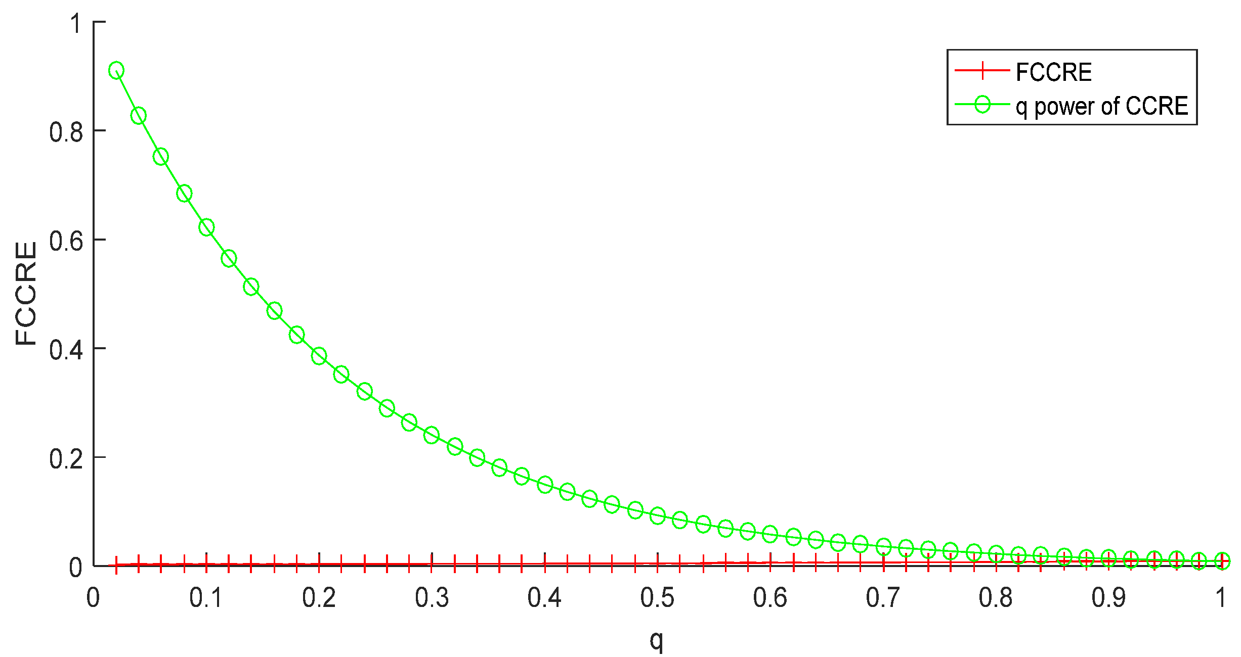
Example 8.

Suppose$U$follows the uniform distribution on$[0, 1]$,$V$follows exponential distribution with$\lambda =0.5$. Figure 10shows the value of${\epsilon }_q\left(U|\eta \right)$is far less than the value of${\left[\epsilon \left(U|\eta \right)\right]}^q$. The larger numerical deviation of FCCRE and q-order CCRE can also be seen from Table 1.

Figure 10. The fractional conditional cumulative residual entropy of ${\epsilon }_q\left(U|\eta \right)$ and the $q$ power of conditional cumulative residual entropy of ${\left[\epsilon \left(U|\eta \right)\right]}^q$.

Table 1. The specific values of q-order FCCRE and q power of CCRE.

	q = 0.1	q = 0.2	q = 0.3	q = 0.4	q = 0.5	q = 0.6	q = 0.7	q = 0.8	q = 0.9	q = 1.0
CCRE	0.0026	0.0027	0.0029	0.0030	0.0031	0.0033	0.0035	0.0036	0.0038	0.0040
q-order FCCRE	0.5752	0.3308	0.1903	0.1094	0.0629	0.0362	0.0208	0.0120	0.0069	0.0040

The following proposition shows that the fractional conditional CRE dominates the differential entropy, which gives a lower bound for the fractional conditional CRE relative to the differential entropy.

Proposition 11.

Let$U\ge 0$have density$f$, then

$${\epsilon }_q\left(U|\eta \right)\ge C_{\left(q\right)}{e}^{H\left(U|\eta \right)},0<q\le 1,$$

(23)

where$H\left(U|\eta \right)$ is the conditional differential entropy defined in Equation (2) [8], and $C_{\left(q\right)}=e^{{\displaystyle {\int }_0^1\log \left[u{\left(-\log u\right)}^q\right]}du}$ is a finite function of $q$.

Proof of Proposition 11.

Let $G\left(U|\eta \right)=P\left[U>u|\eta \right]={\displaystyle {\int }_u^{\infty }f\left(u|\eta \right)}$, using the log-sum inequality,

$$\begin{gathered} {\displaystyle {\int }_u^{\infty }f(u\left|\eta \right.)\log \frac{f(u\left|\eta \right.)}{G(u\left|\eta \right.){\left[-\log G(u\left|\eta \right.)\right]}^q}}du\ge \log \frac{1}{{\displaystyle {\int }_0^{\infty }G(u\left|\eta \right.){\left[-\log G(u\left|\eta \right.)\right]}^{q}du}} \\ =\log \frac{1}{{\epsilon }_q(u\left|\eta \right.)}. \end{gathered}$$

(24)

The LHS in Equation (24) equals

$$-H(U\left|\eta \right.)-{\displaystyle {\int }_0^{\infty }f(u\left|\eta \right.)\log \left[G(u\left|\eta \right.){\left[-\log G(u\left|\eta \right.)\right]}^q\right]du}.$$

Then

$$H(U\left|\eta \right.)+{\displaystyle {\int }_0^{\infty }f(u\left|\eta \right.)\log \left[G(u\left|\eta \right.){\left[-\log G(u\left|\eta \right.)\right]}^q\right]du}\le \log {\epsilon }_q(U\left|\eta \right.).$$

(25)

Finally, a change in variable gives

$${\displaystyle {\int }_0^{\infty }f(u\left|\eta \right.)\log \left[G(u\left|\eta \right.){\left[-\log G(u\left|\eta \right.)\right]}^q\right]du}={\displaystyle {\int }_0^1\log \left[u{(\log u)}^q\right]}du.$$

Hence, we obtain the following equation from Equation (25):

$$H\left(U|\eta \right)+{\displaystyle {\int }_0^1\log \left[u{\left(-\log u\right)}^q\right]}\le \log {\epsilon }_q\left(U|\eta \right).$$

(26)

Exponentiating both sides of Equation (26), we have Equation (23). □

Definition 2.

Cross CRE [8] is defined as

$$\epsilon \left(U,V\right)=\epsilon \left(U\right)+E\left[\epsilon \left(V|U\right)\right].$$

(27)

Similarly, we define fractional cross CRE by

$${\epsilon }_q\left(U,V\right)={\epsilon }_q\left(U\right)+E\left[{\epsilon }_q\left(V|U\right)\right].$$

(28)

Now, using Proposition 11, we have the following proposition.

Proposition 12.

$${\epsilon }_q\left(U,V\right)\ge 2C_q\exp \left(\frac{H\left(U,V\right)}{2}\right),$$

(29)

where$H\left(U,V\right)$is the joint entropy [1].

Proof of Proposition 12.

The combination of Proposition 11, the convexity of $e^x$, and Jensen’s inequality lead to

$$\begin{gathered} {\epsilon }_q\left(U,V\right)={\epsilon }_q\left(U\right)+E\left[{\epsilon }_q\left(V|U\right)\right] \\ \ge C_q\exp \left[H\left(U\right)\right]+C_q\exp \left[H\left(U|V\right)\right] \\ \ge 2C_q\exp \left\{\frac{H\left(U\right)+E\left[H\left(U|V\right)\right]}{2}\right\} \\ =2C_q\exp \left\{\frac{H\left(U|V\right)}{2}\right\}. \end{gathered}$$

In the second inequality, we use $2\exp \left\{\frac{u+v}{2}\right\}\le e^u+e^v$. □

4. Empirical Fractional Conditional Cumulative Residual Entropy

Analogous to CRE, conditional FCRE can be computed using the fractional CRE of empirical data [30,31,32,33].

Let $U_1,U_2,\cdots ,U_n$ be nonnegative absolutely continuous, independently and identically distributed random variables that form a random sample from a population having distribution function $F(U|v)$ for an $\sigma$-field $\eta$, which is generated by a random variable $V$. Writing $F_n\left(U|v\right)$ as the empirical conditional distribution of n-sample $U_1,U_2,\cdots ,U_n$, assigning mass $\frac{1}{n}$ to every sample point, then $F_n\left(U|v\right)$ is the conditional cumulative distribution function.

According to Equation (4), the CRE of empirical distribution $F_n\left(U|v\right)$ is

$${\epsilon }_q\left({\overline{F}}_n\left(U|v\right)\right)={\displaystyle {\int }_0^{\infty }{\overline{F}}_n\left(U|v\right){\left[-\log {\overline{F}}_n\left(U|v\right)\right]}^{q}du},$$

(30)

where ${\overline{F}}_n\left(U|v\right)$$=1-F_n\left(U|v\right)$.

The following propositions uncover the asymptotic of empirical fractional conditional CRE, namely the FCCRE of sample data asymptotically converges to the true value.

Proposition 13.

For any random variable$U$in$L^p$for some$p>1$, empirical conditional FCRE converges to the conditional FCRE of$U$, i.e.,${\epsilon }_q\left[F_n\left(U|v\right)\right]\to {\epsilon }_q\left[F\left(U|v\right)\right]$a.s.

Proof of Proposition 13.

By using the dominated convergence proposition, it holds that the integral of $G_n\left(U|v\right)\log G_n\left(U|v\right)$ on any finite interval converges to that of $G\left(U|v\right)\log G\left(U|v\right)$. Therefore, we just need to show that as $n\to \infty$

$$\left|{{\displaystyle {\int }_0^1{G}_n(U\left|v\right.)\left[-\log G_n(U\left|v\right.)\right]}}^{q}du-{{\displaystyle {\int }_0^{1}G(U\left|v\right.)\left[-\log G(U\left|v\right.)\right]}}^{q}du\right|\to 0.$$

Recall that

$$G_n\left(U|v\right)=P_n\left(U>u|v\right),$$

where $P_n$ is the probability distribution on $R_{+}$ assigning mass $\frac{1}{n}$ to each of the sample points $U_1,\cdots ,U_n$.

It follows that

$$x^p{G}_n\left(U|v\right)\le E_n\left[U^P\right]=\frac{1}{n}{\displaystyle \sum _1^n{U}_j^p},$$

(31)

where $E_n$ is expectation relative to $P_n$. Then, using the strong law [28], we obtain

$$\frac{1}{n}{\displaystyle \sum _1^n{U}_j^p}\to E\left[U_1{}^P\right] \mathrm{almost} \mathrm{surely}.$$

(32)

In particular,

$$\underset{n}{\sup }\frac{1}{n}{\displaystyle \sum _1^n{U}_j^p<\infty } \mathrm{almost} \mathrm{surely}.$$

Combining Equations (31) and (32), we obtain $G_n\left(U|v\right)\le u^{-p}\left(\underset{n}{\sup }\frac{1}{n}{\displaystyle \sum _1^n{U}_j^p}\right)$

Now, by applying the dominated convergence proposition and using Equation (35) in Ref. [8], we prove the proposition. □

Proposition 14.

Let the random vector$U_n$converge to the random vector$U$in distribution for all bounded continuous functions$\phi$on$R_N$, that is

$$\underset{n\to \infty }{\lim }E\left[\phi \left(U_n\right)\right]=E\left[\phi \left(U\right)\right].$$

For some$p>N$,if all the$U_n$are bounded in$L^p$, then

$${\epsilon }_q\left(U_n|v\right)\stackrel{a.s.}{\to }{\epsilon }_q\left(U|v\right),n\to \infty .$$

Proof of Proposition 14.

For all $u$ on $R_N^{+}$, $U_n$ converges to the random vector $U$ in distribution [29],

$$\underset{n\to \infty }{\lim }P\left[\left|U_n\right|>u|v\right]=P\left[\left|U\right|>u|v\right].$$

Then, for all $u$,

$$\underset{n\to \infty }{\lim }P\left[\left|U_n\right|>u|v\right]\log P\left[\left|U_n\right|>u|v\right]=P\left[\left|U\right|>u|v\right]\log P\left[\left|U\right|>u|v\right].$$

From Proposition 1 in Ref. [8], we know

$${\left[P\left[\left|U_n\right|>u|v\right]\left|\log P\left[\left|U_n\right|>u|v\right]\right|\right]}^q\le {\left(\frac{e^{-1}}{1-\alpha }\right)}^q{\left[{\displaystyle \prod _{j=1}^{N}P{\left[\left|U_{n_j}\right|>U_j|v\right]}^{\raisebox{1ex}{$\alpha $}\!\left/ \!\raisebox{-1ex}{$N$}\right.}}\right]}^q.$$

For each $n$ and $j$,

$$\begin{gathered} {\displaystyle {\int }_0^{\infty }P{\left[\left|U_{n_j}\right|>U_j|v\right]}^{\raisebox{1ex}{$q\alpha $}\!\left/ \!\raisebox{-1ex}{$N$}\right.}du}={\displaystyle {\int }_0^{1}P{\left[\left|U_{n_j}\right|>u_j|v\right]}^{\raisebox{1ex}{$q\alpha $}\!\left/ \!\raisebox{-1ex}{$N$}\right.}+{\displaystyle {\int }_1^{\infty }P{\left[\left|U_{n_j}\right|>u_j|v\right]}^{\raisebox{1ex}{$q\alpha $}\!\left/ \!\raisebox{-1ex}{$N$}\right.}du}} \\ \le 1+{\displaystyle {\int }_1^{\infty }{\left\{\frac{1}{u_j^p}E{\left[\left|U_{n_j}\right||v\right]}^p\right\}}^{\raisebox{1ex}{$q\alpha $}\!\left/ \!\raisebox{-1ex}{$N$}\right.}du}, \end{gathered}$$

where $\frac{pq\alpha }{N}>1$, the proposition can be proved. □

5. Application

In this section, we analyze and compare the complexity of aero-engine gas path variables based on the FCRE and FCCRE models, so as to explore the intrinsic dynamic nature of aero-engine time series. We select the engine pressure ratio (EPR), high-pressure rotor speed (N1), fuel flow (WF), and exhaust gas temperature (EGT) as data samples. These four major variables reflect the operation condition of the aero-engine gas path system.

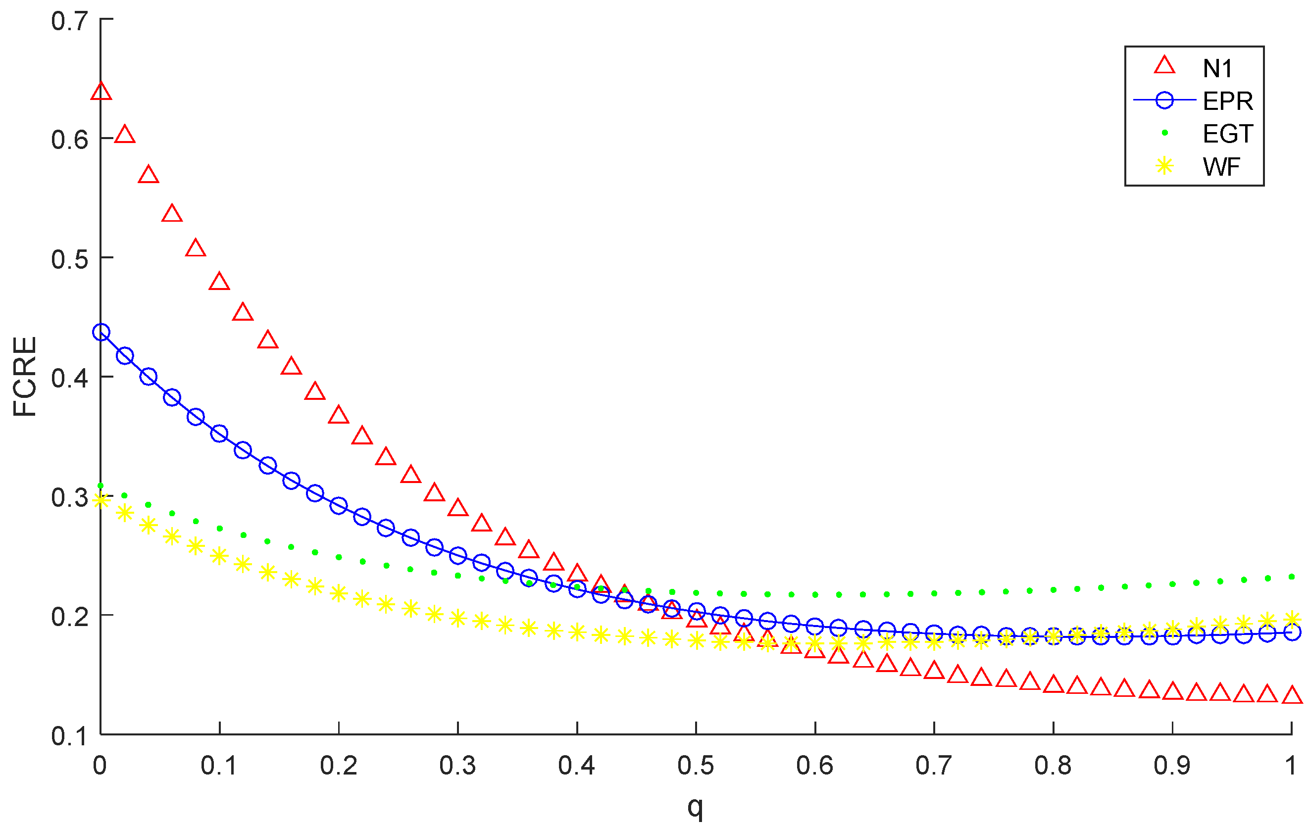
The fractional cumulative residual entropy curves of the six groups series in Figure 11 are interlaced to varying degrees and show a decreasing trend with the increase in fractional parameters. Through fractional parameter analysis, we can explore the inherent dynamic nature of aero-engine gas path time series and try to distinguish different gas path parameters. In Figure 11, the entropy curve of N1 (high pressure rotor speed) is higher than that of the EPR (engine pressure ratio), WF (fuel flow), and EGT (exhaust gas temperature) while $\mathrm{q}\le 0.4$. Oppositely, when $\mathrm{q}\ge 0.6$, the entropy curve of N1 lies under that of the EPR, WF, and EGT. The reason may be that N1 represents the dynamic system. However, the oiling system and temperature system associated with the dynamic system are indicated by the WF and EGT.

Figure 11. The fractional cumulative residual entropy of N1, EGT, EPR, and WF time series.

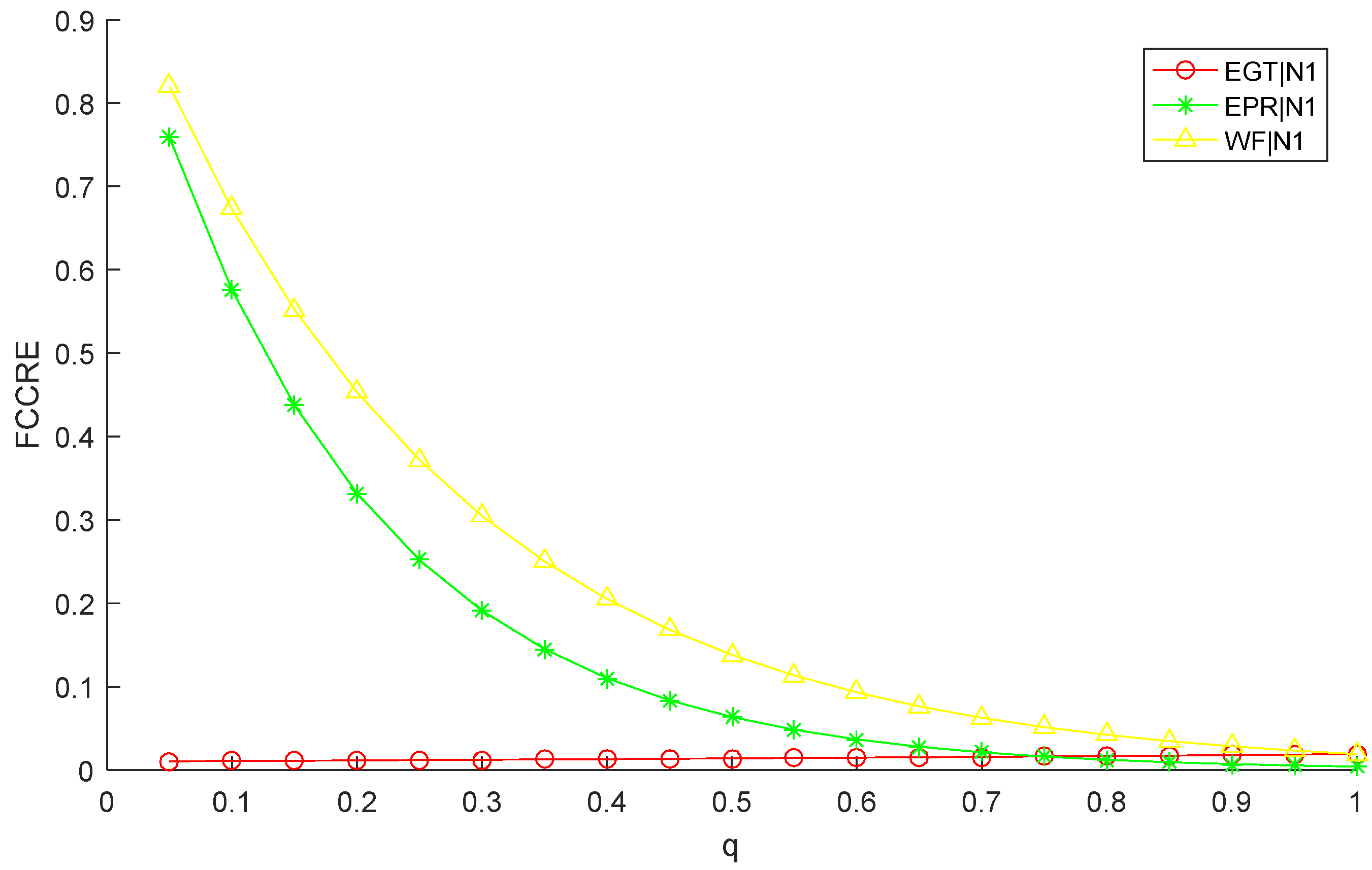
In order to better observe the correlation between the dynamic system and three other systems, Figure 12 shows the FCCRE of these three groups of gas path sequences, respectively. Figure 12 shows a wide difference in the correlation for the aero-engine gas path time series. The FCCRE values of the ${\mathsf{\epsilon }}_{\mathrm{q}}\left(\mathrm{EGT}\left|\mathrm{N}1\right.\right)$ and ${\mathsf{\epsilon }}_{\mathrm{q}}\left(\mathrm{EPR}\left|\mathrm{N}1\right.\right)$ sequences firstly decrease rapidly with the increase in parameter q, and then decrease slowly. On the other hand, when q increases, the entropy curve is obviously near the highest point.

Figure 12. The fractional conditional cumulative residual entropy of aero-engine gas path time series.

In summary, both FCRE and FCCRE can detect the nature of gas path systems and can distinguish the complexity of different gas path series. The result of FCCRE can capture not only the information of complexity but also the correlation in the gas path system.

6. Conclusions

In this paper, some new properties of fractional cumulative residual entropy and fractional conditional cumulative residual entropy (FCCRE) were given. Among them, some properties revealed the connection between fractional conditional CRE and differential entropy. Moreover, the generated random sequences that followed different distributions were used to verify the validity of the original property. Then, we discussed the empirical approximation of FCCRE.

For the analysis of aero-engine gas path data, this article analyzed and compared the complexity of the engine pressure ratio (EPR), high-pressure rotor speed (N1), fuel flow (WF), and exhaust gas temperature (EGT). The results show that both FCRE and FCCRE can detect the complex nature of the gas path system. In the future, we will continue to investigate other properties and applications of fractional-order cumulative residual entropy and fractional conditional cumulative residual entropy.