Article

Fractal Description of Rock Fracture Networks Based on the Space Syntax Metric

1
College of Science, North China University of Technology, Beijing 100144, China
2
College of Petroleum Engineering, Northeast Petroleum University, Daqing 163318, China
3
School of Safety Engineering, North China Institute of Science and Technology, Sanhe 065201, China
4
School of Civil and Resource Engineering, University of Science and Technology Beijing, Beijing 100083, China
5
College of Science, North China Institute of Science and Technology, Beijing 101601, China
*
Authors to whom correspondence should be addressed.
Fractal Fract. 2022, 6(7), 353; https://doi.org/10.3390/fractalfract6070353
Submission received: 7 April 2022 / Revised: 13 May 2022 / Accepted: 17 May 2022 / Published: 23 June 2022
(This article belongs to the Special Issue Applications of Fractal Geometry Theory in Porous Media)

Abstract

:
Fractal characteristics and the fractal dimension are widely used in the description and characterization of rock fracture networks. They are important tools for coal mining, oil and gas transportation, and other engineering problems. However, due to the complexity of rock fracture networks and the difficulty in directly applying the limit definition of the fractal dimension, the definition and application of the fractal dimension have become hot topics in related projects. In this paper, the traditional fractal calculation methods were reviewed. Using the traditional fractal theory and the head/tail breaks method, a new fractal dimension quantization model was established as a simple method of fractal calculation. This simple method of fractal calculation was used to calculate the fractal dimensions of three rock fracture networks. Through comparison with the box-counting dimension calculation results, it was verified that the model could calculate the fractal dimension of the fracture length of rock fracture networks, as well as quantify it accurately and effectively. In addition, we found a number of similarities between rock fracture networks and urban road traffic networks in GIS. The application of the space syntax metric to rock fracture networks prevents controversy with respect to the definition of the axis and it showed a good effect. Using the space syntax metric as a parameter can better reflect the space relationship of rock fractures than length. Through the calculation of the fractal dimension of the connection value and control value, it was found that the trend of the length fractal dimension was the same as that of the control value, whereas the fractal dimension of the connection value was the opposite. This further verifies the applicability of the space syntax metric in rock fracture networks.

1. Introduction

Under the action of long-term crustal movement, natural erosion, and artificial fracturing, a large number of rock fracture networks with different scales have been formed in rocks [1,2]. According to the research of scholars and experts, rock fracture networks are widely used as the migration channels and collection locations of important strategic resources such as gas, natural gas, shale gas, and oil [3,4,5]. They are also used in disaster warning, mine safety, engineering geology, and other fields [6,7]. As such, quantifying rock fractures is important in these fields. According to studies over the last few decades, many different methods have been found to characterize rock fracture networks. For example, Li et al. used probability weighted moments and L-moments to estimate and describe the distribution of fracture length trajectories [8]. In another study, Lu et al. analyzed and evaluated the striking of natural fractures [9]. Furthermore, many experts have analyzed rock fracture porosity and dip amplitudes while studying rock fracture networks [10,11]. Because rock fractures span many scales and exist in a wide range, descriptions of the overall level of fracture for certain scales are incomplete [12]. In addition to these traditional geometry methods, the self-similarity of rock fracture networks at different scales, i.e., fractal geometry, has become one of the most suitable methods for the quantitative study of rock fracture networks [13,14,15,16,17,18].
Since Barton first used fractal geometry to quantify a two-dimensional rock fracture network, fractal geometry has been widely used to describe rock fracture networks. By using the fractal dimension, Silberschmidt accounted for the stochastic nature of mechanical properties and their effect on the process of fracture development [19]. Koike proposed a method to estimate the existence probability of fractures longer than a defined length and found fractal characteristics in both the fracture direction and the trace length [20]. Zhou et al., according to fractal geometry theory, integrated microseismic and well production data for fracture network calibration [21]. Huang et al. used fractal porosity and permeability to describe the nonuniform distribution of a complex fault network [17]. Liu and Yu considered the influence of the fracture pore structure, constructed a multifield coupling mechanical model, and further studied the fractal dimension evolution mechanism of coal seam fractures [22]. Riley applied the correlation dimension to quantitatively quantify the fracture spacing of nonlayered rocks. They proposed that the correlation dimension provided a more rigorous mathematical calculation than other fractal methods used in structural geology and is particularly stable in the case of limited data [15]. Some scholars not only used fractal geometry to quantify rock fractures, but also applied it to practical engineering, obtaining good engineering benefits. For example, Mecholsky found that there was a correlation between the fractal dimension of the fracture surface and the toughness [23]. Using fractal geometry, Sheng et al. proposed a new method to evaluate the effective stimulated reservoir volume of a shale reservoir, which was successfully applied [24]. Subsequently, Geng established a fractal production prediction model of a shale gas reservoir [14].
Previously, Sui used fractal geometry to describe the fracture degree of shale. Their research results showed that the fractal dimension of the fracture network could be used to guide the evaluation model of shale fracability; they found that more complex fractures resulted in greater shale fracability [25]. Although the fractal dimension has been widely used in the quantification of rock fracture networks, some disputes remain as to whether this application is correct or not. Gillespie et al. analyzed one-dimensional and two-dimensional rock fault joints using fractal theory and determined that the regular spacing of a single-direction joint set did not satisfy the fractal characteristics; hence, they determined that the rock fault was nonfractal [26]. Walsh et al. obtained a nonlinear box-counting curve, and they determined the rock fracture mode to be nonfractal [27]. Some researchers used a variety of methods to calculate the fractal dimension of images and they found that the effects, and even the changing trends of the fractal dimension, were not the same [28]. The reason for these differing opinions on the application of the fractal dimension in rock fracture networks is that the original definition of the fractal dimension required strict self-similarity—which does not exist in nature. In addition, in the past, the calculation of the fractal dimension in the past often involved using the least-squares method to determine the limit, whereby the approximate value was not sufficiently effective or accurate; thus, a tiny difference in the fractal dimension would appear in engineering applications. Lastly, using only the length fractal dimension is too simple an approach to describe the complexity of the whole rock fracture network space.
Based on the latest fractal definition, in this paper, an effective and accurate calculation method of fractal dimension is established. The limit calculation is removed, and more space syntax parameters are used to measure the fractal dimension of different fracture properties, which can accurately represent the spatial relationship of fractures, for calculation and quantification. This paper is divided into six parts: after the introduction, the second part introduces the basic concept of the space syntax metric and analyzes the relationship between the space syntax metric and rock fracture networks. The third part analyzes the traditional fractal calculation method, considering the existing problems and combining the head/tail breaks method, and proposes the simple method of fractal calculation. In the fourth part, three real rock fracture maps are analyzed and calculated using the new fractal calculation method. The results are compared with the box-counting method and the effectiveness of the calculation method is verified. In the fifth part, the head/tail breaks method is used to screen the extracted space syntax metric. The connection and control values are then selected to calculate and analyze both the fractal dimension and length fractal dimension. The results show that the trend of fractal dimension of length is the same as that of the control value; however, it is opposite to that of the connection value. The sixth part summarizes the whole paper.

2. Space Syntax Metrics

2.1. The Concept of Space Syntax Metrics

Measuring space objects is one of the most basic functions of GIS (Geographic Information System). Space syntax was originally developed by Bill Hillier and his colleague Julienne Hanson. Space syntax provides a group of theories and methods for the analysis of spatial configurations of all kinds and at all scales [29]. There are four components of space syntax—representations of space, analysis of spatial relations, interpretive models, and the theories of the relations between spatial and social patterns [30]. The structure and relationships between spatial elements resulting from their configuration are studied in space syntax, which makes it feasible for analyzing how rock network geometrics form due to their similar spatial characteristics. Space syntax mainly uses the longest visibility line to represent the axis, and then gathers the axis sets in the space to form an axis diagram [31]. However, the definition of axis has always been controversial, because some curved routes and the influence of external factors on the road will cause the axis to not be well expressed. For example, Robert C. Thomson took the line segment in the smooth continuous road as the basis for analyzing the street and road network and argued that this method can measure the road network more effectively and robustly [32]. Based on the principle of good continuity and completeness, Xintao Liu generated the axis diagram of a natural city with the minimum set of independent straight-line segments intersecting each other along the natural streets as the axis and proved that the newly defined axial line is a better choice for capturing the potential urban structure [33].
After selecting the appropriate definition axis and establishing the preliminary axis diagram, the next step is using graph theory, geometry, and topology to analyze and improve the axis diagram to form a complete natural urban road network. Finally, a series of space syntax variables are selected for spatial analysis—the connection variable is derived to represent the number of spaces intersected by a certain space in the system; control represents the control degree of the space intersected by a certain space, which is numerically equal to the sum of the reciprocal of the connection values of the adjacent spaces; depth is the minimum number of connections that a space needs to go through to reach other spaces; and integration is the degree of agglomeration or dispersion between one space and other spaces in the system. For example, Bin Jiang analyzed the network streets of large cities with a topological method and calculated a series of space syntax metrics for structural analysis, including street connectivity, average path length, and the clustering coefficient [34]. Subsequently, Jiang et al. used a large number of road network and traffic network flow data to analyze the relationship between the line-based method and the point-based method and concluded that the point-based method was the most suitable choice [35]. In another study, Sang Kyu Jeong developed a topology information extraction model (TIEM) to extract basic information from the building information created by a CAD (Computer aided design) system and to automatically identify or recognize the geometric and topological features of space, so as to better carry out space syntax analysis [36].

2.2. The Relationship between Space Syntax Metrics and Rock Fracture Networks

Space syntax has proven to be a valuable tool for simulating and analyzing urban road traffic networks related to human activities. For example, Bin Jiang carried out a topological representation and prediction analysis of traffic flow based on the space syntax measurement of street networks [37], whereas Faris Ali Mustafa evaluated primary school buildings in Erbil City using space syntax analysis and schoolteacher feedback [38]. However, the definition of the axis has always been controversial, and we cannot find a perfect definition that accurately represents the axis in urban spaces. If the axis is defined by the rock fractures in the rock fracture network—and because there are no external factors such as pedestrian flow, vehicle flow, or buildings—disputes over the definition will disappear. Moreover, the rock fracture network has the same characteristics as the urban road network (such as self-similarity, heavy-tailed distribution, being scale-free, and so on). Therefore, it is rational to identify and analyze the rock fracture network using space syntax.

3. Methodology

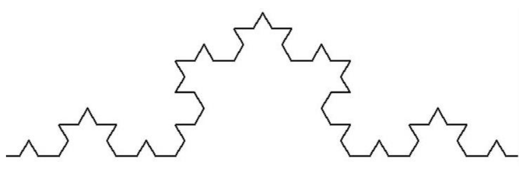
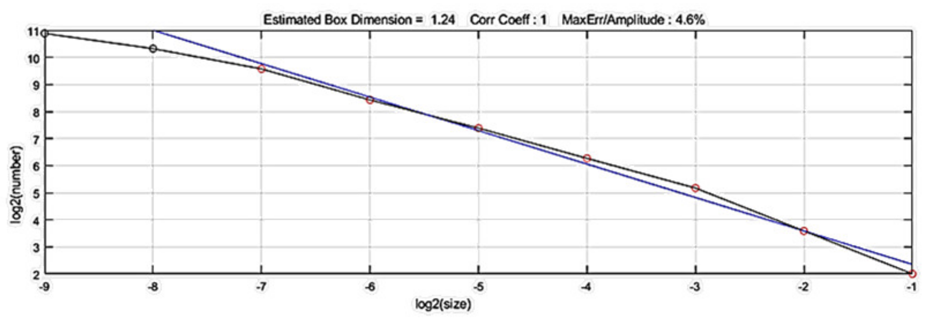
3.1. Traditional Fractal Calculation Method

In traditional geometry, people usually use Euclidean geometry based on the Cartesian coordinate system to describe objects. However, with the development of science and technology, it has been found that Euclidean geometry cannot describe certain irregular objects, such as a curved coastline, rugged mountains, or crisscross rock fissures. When Mandelbrot published his papers in 1967, the idea of using fractals to quantitatively describe irregular objects appeared. However, it was not until 1982 that the theoretical system of fractal geometry was formed. Many experts and scholars began to use fractal geometry to describe irregular objects with self-similar hierarchical structures that cannot be described by Euclidean geometry. Xu Peng, Zheng Qian, and Shen Yuqing, along with other scholars, applied fractal geometry to porous media. They established a prediction model for liquid flow and gas diffusion in porous media [39,40,41]. In a series of studies, Yu Boming and colleagues established a fractal permeability model, also for porous media, based on the fractal characteristics of pores in the medium. The experimental data were in good agreement with the actual data, which also proved the practicability of fractal geometry in practical engineering [42,43,44].
In recent years, scholars have established a variety of methods for calculating fractal dimensions, among which the most commonly used are the correlation dimension method and the box-counting dimension method. The box-counting dimension method is based on measuring distance in space. The fractal is placed on an evenly divided grid, and the box-counting dimension is calculated using the ratio of the logarithm of the number of grids to the logarithm of the reciprocal of the grid edge length. The smaller the grid edge length, the more accurate the calculation result [26]. In this paper, the box dimension of the fractal is calculated using the FRACLAB toolbox in MATLAB (2018a, MathWorks, Inc., Portola Valley, CA, USA), taking the Koch curve shown in Figure 1 as an example:
First, the program is written to distinguish the fractal region from the background to reduce the noise—that is, to convert the RGB (red, green, blue) image from three-dimensional data into a two-dimensional matrix. For the binary image, the white area is 1, the black area is 0, and the image is a black line with a white background which we need to reverse for subsequent operation. The obtained image is shown in Figure 2.
Then, the dimension of the Koch curve is calculated by using FRACLAB toolbox. According to the size of the picture, nine types of boxes (with an upper limit of 1/2 and a lower limit of 1/512) are automatically generated. The progressive relationship of the box size is a power law. According to the appropriate correlation coefficient and maximum error, the range of the fitting curve is selected, and the final fractal dimension is obtained. As shown in Figure 3, the theoretical value of the fractal dimension of the Koch curve is 1.2619 and the test value calculated by MATLAB (2018a) is 1.24. The difference between the two is small, and the error is only 1.7%. Therefore, this method can be used to calculate the box-counting dimension.

3.2. A Simple Method of Fractal Calculation

For the most commonly used fractal dimensions, such as the box-counting dimension method and the correlation dimension method, the least-squares method is used for fitting; however, the fitting results are unstable and distorted [45]. Based on the hierarchical structure of fractal long-tail distribution and the self-similarity between local and global, Bin Jiang proposed the HT (head/tail) index based on the head/tail breaks method to supplement the fractal dimension—which could avoid strict-limit algorithms in computation [46]. The basic concept is as follows: taking the average length of the figure as the median, the figure is divided into two parts; the part larger than the median is the head and the part smaller than the median is the tail. If the proportion of the head is less than the threshold value, the head is segmented continuously, and the number of segmentations plus 1 is the HT index. As shown in Figure 4, for a Koch curve with three iterations, when there is an increase in iterations, the HT index gradually increases, while the fractal dimension remains unchanged. For the same iteration number, when there is an increase in the length of the middle two sections, the fractal dimension gradually increases, while the HT index remains unchanged. The HT index captures certain characteristics that cannot be captured by the fractal dimension, making it a good supplement to the fractal dimension [47]. In addition, the concept of the fractal is greatly expanded based on the HT index, and a new definition is given. As such, if the HT index of a graph is at least three, it is considered to be a fractal. In this way, there is a new problem. Some HT indexes are determined to be fractals with this new definition; however, the exact fractal dimension cannot be calculated using the previous calculation method. Therefore, it is necessary to establish a new fractal dimension calculation formula according to the new definition.
Fractal theory comes from the expansion of our traditional geometry. The definition of the Euclidean dimension is generalized. When we increase the length of each side of a square to three times that of the original, the big square is exactly equal to 32 = 9 original squares. Similarly, when we increase the length of each side of a cube by three times, the big cube is equal to 33 = 27 original small cubes. If we generalize this, each independent direction of a d-dimensional geometric object is increased by a factor of one. As a result, N original objects are obtained, which satisfy the following relation: l d = N . It is not difficult to verify that this simple relation is true for all ordinary geometric objects in Euclidean geometry. Taking logarithms on both sides of this relation, we can obtain D = ln N ln l . In Euclidean geometry, all topological dimensions D are integers. However, if we take this relation as the definition of the fractal dimension and do not restrict it by rounding, we can obtain the generalized definition of the fractal dimension [49], which is represented by the capital letter D:  D = lim l 0 ln N ln l , where N is the number of self-similar sets and l is the scale ratio of self-similar sets.
When using HT to segment the fractal set, the head of each segmentation is a similar fractal set to the original fractal set. We combine the traditional definition of a fractal with the method of head/tail breaks, take the ratio of the number of heads and tails as the number of fractal sets, and then take the ratio of the average value of the heads and tails as the scale ratio of fractal sets, considering the average effect of all the HT breakings. The current fractal dimension calculation method is thus expanded, and the average value of each HT-breaking fractal dimension algorithm is applied to describe the overall fractal characteristics. This method’s formula is:
D = 1 n 1 1 n ln N t i / N h i ln M t i / M h i ,
where N h i is the number of fractures in the head of the i th breaking, N t i is the number of fractures in the tail of the i th breaking, M h i is the average measure of the value of the heads in the i th breaking, and M t i is the average value of the tail of the i segmentation. In addition, the 40% threshold used in HT breaking is also limited in real data and can be adjusted according to different fractal sets [50]. For example, the two most commonly used laws in the life structure—scale law and Tobler law—adopt 20% and 50% thresholds to break things, respectively [51].

4. Comparison between Box-Counting Dimension Method and the Simple Method of Fractal Calculation

In this part, we use the box-counting dimension method and the simple method of fractal calculation to calculate the fractal dimensions of three rock fracture network diagrams. These diagrams are used to compare and verify the effectiveness of the simple method of fractal calculation. First, for a, b, and c, from left to right, as shown in Figure 5, Figure 6 is obtained by inversing the three rock fracture network diagrams. Then, the box-counting dimension of the inversed rock fracture network diagram is calculated using the FRACLAB toolbox in MATLAB (2018a), which uses the box-counting dimension calculation method discussed in Section 3.1. The results are shown in Figure 7.
It can be seen from Figure 7 that the fractal dimensions of the three rock fracture network diagrams are 1.79, 1.7, and 1.63, respectively. Next, the fractal dimensions of rock fracture networks is calculated using the simple method of fractal calculation. First, the length data of the rock fracture networks are extracted for the head/tail breaks, and the results are shown in Table 1.
It can be seen from Table 1 that the HT indexes of the three rock fracture network diagrams are 6, 6, and 6, respectively. According to the new definition of fractal dimensions, an HT index of no less than 3 can be considered to be a fractal, meaning that the fractal dimensions of the three rock fracture networks can be calculated. According to the data in Table 1, the calculation results of the fractal dimensions of the rock fracture networks are as follows:
D h = 1 4 ln 276 138 ln 10.34 47.25 + ln 98 40 ln 33.88 80 + ln 27 13 ln 62.11 117.15 + ln 8 5 ln 97.5 148.6 + ln 4 1 ln 136 199 = 1.852 ,
D i = 1 4 ln 167 94 ln 8.98 38.15 + ln 66 28 ln 26.67 65.21 + ln 19 9 ln 50.05 97.22 + ln 6 3 ln 77.33 137 + ln 2 1 ln 126 159 = 1.668 ,
D j = 1 4 ln 92 47 ln 13.23 57.19 + ln 30 17 ln 39.63 88.18 + ln 10 7 ln 65.7 120.29 + ln 4 3 ln 100.25 147 + ln 2 1 ln 129 183 = 1.498 .
The fractal dimensions of the rock fracture networks are 1.852, 1.668, and 1.498. It can be seen that the order of the fractal dimensions and the complexity of rock fractures are the same as those of the box-counting dimension, which proves the effectiveness of this method.

5. Comparison of Metric Parameter of Space Syntax and Length Fractal Dimension

In this part, we compare and calculate the dimension parameters of space syntax and the length fractal dimension. To extract the space syntax metric data of rock fracture networks, we used the Axwoman plug-in in ArcGIS (ArcGIS 10.2, Esri, Redlands, CA, USA). First, the axis drawing function was used to draw rock fractures along the fracture direction, with any point as the starting point and the connecting point between the fracture and other fractures as the end point, until the whole rock fracture network diagram was drawn. Then, the function for tracking a natural street was used to integrate the network graph of the rock fracture with topological geometry information. If the rock fracture was connected to two or more other rock fractures, the rock fracture that had an extension line with less than a 45-degree angle was regarded as the same rock fracture; if more than one rock fracture had an extension line with less than a 45-degree angle, the longer line was selected as the same fracture [45]. Finally, the computational geometry function was used to calculate all fracture length attributes. Seven kinds of space syntax parameters and length data were derived. Since the calculation of space syntax requires the deletion of isolated fractures, the following calculation involved deleting the parameters of isolated fractures.

5.1. Parameter Selection

According to the total number of rock fractures, the syntactic measures of the fracture space were extracted. These are the connection value, control value, average depth value, global depth value, local depth value, global integration degree, local integration degree, and the length value of the rock fractures. First, taking Figure 6c as an example, power law analysis (Figure 8) and the HT index calculation (Table 2) were carried out for eight kinds of extracted data. The results are as follows:
It can be seen from Figure 8 that only the length value, the connection value, and the control value meet the fractal requirements. According to the data in Table 2, the length value, connection value, and control value of the HT index were greater than 3, satisfying the new fractal dimension determination. Therefore, we chose two space syntax parameters—the connection value and the control value—to calculate and compare the length fractal dimension.

5.2. Comparison of Fractal Dimension Calculation

The length value, connection value, and control value of a, b, and c rock fracture diagrams are calculated using Formula (1)
D 8 a c o n n e c t = 1.012 ,   D 8 a C o n t r o l = 1.447 ,   D 8 a l e n g t h = 1.843 .
D 8 b c o n n e c t = 1.39 0 ,   D 8 b C o n t r o l = 1.390 ,   D 8 b l e n g t h = 1.566 .
D 8 c c o n n e c t = 1.675 ,   D 8 c C o n t r o l = 1.238 ,   D 8 c l e n g t h = 1.084 .
Through the calculation of the fractal dimensions of the connection value and the control value of the three rock fracture networks, it was found that the fractal dimensions of the length and control values had the same trend, while the fractal dimensions of the connection value were the opposite. The connection value and the control value both represent the relationship between a certain space and a space directly connected to it. The connection value indicates how many other axes of the axis itself are connected to it, while the control value indicates the reciprocal sum of the connection values of the other axes connected to the axis; therefore, the control value of an axis with a high connection value is not necessarily high. Because some axes may have high connection values, the connection value of the axis connected to them is also very high, inevitably leading to a low control value. In hydraulic fracturing engineering, a fracture network with a higher fractal dimension of length is more complex, and its fracability is higher, whereas the permeability of a rock fracture with lower connectivity is higher and the fracturing effect is better, which is completely consistent with our calculation results. Compared with using the length fractal dimension as a parameter, using the connection value and the control value as parameters to calculate the fractal dimension can better reflect the spatial characteristics of rock fracture networks. Moreover, it can also provide a number of ideas to researchers in the field of fractal dimensions and rock fracture networks.

6. Conclusions

Through analysis of the space syntax metric, it was found that the metric can be well applied to rock fracture networks. By discussing and analyzing a number of problems in the existing fractal dimension calculation methods, a new fractal dimension calculation method was proposed based on traditional fractal theory and head/tail breaks. Using the simple method of fractal calculation, the fractal dimensions of three rock fracture networks were calculated and compared with the box-counting dimension, which verified the accuracy and effectiveness of the model. In addition, through the calculation of the fractal dimensions of some space syntax metrics, the applicability of the space syntax measures, and rock fracture networks was verified. The main conclusions are as follows:
(1)
Based on the characteristics of self-similarity, heavy-tailed distribution, and being scale-free between the urban street networks and the rock fracture networks, we found that the space syntax metric of the urban street network can be effectively applied to rock fracture networks. Taking the rock fractures as the axis, there would be no dispute about the definition of the axis, which could better show the spatial structure of rock fracture networks.
(2)
Based on the traditional fractal theory and the head/tail breaks method, we proposed a new fractal dimension calculation method. The calculation process does not take the limit operation into consideration; the results are more stable than the previous fractal dimension calculation method. Because it combines the HT index and the traditional fractal dimension idea, the new calculation method can better and more effectively capture the fractal characteristics of a fractal set.
(3)
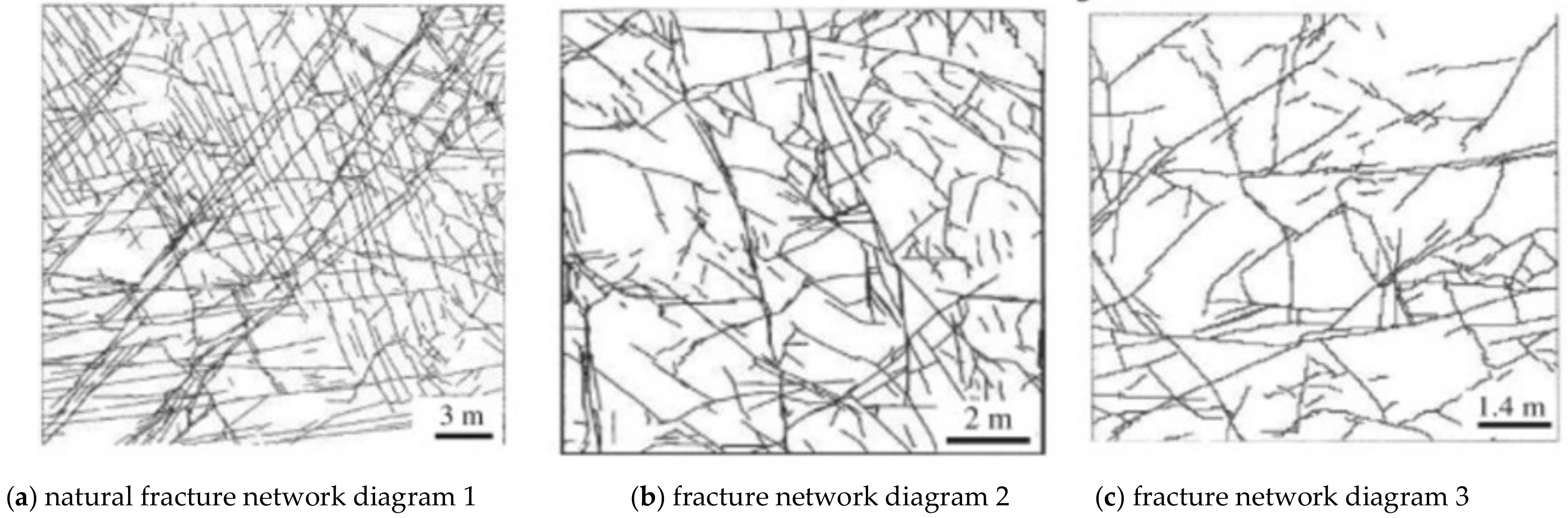
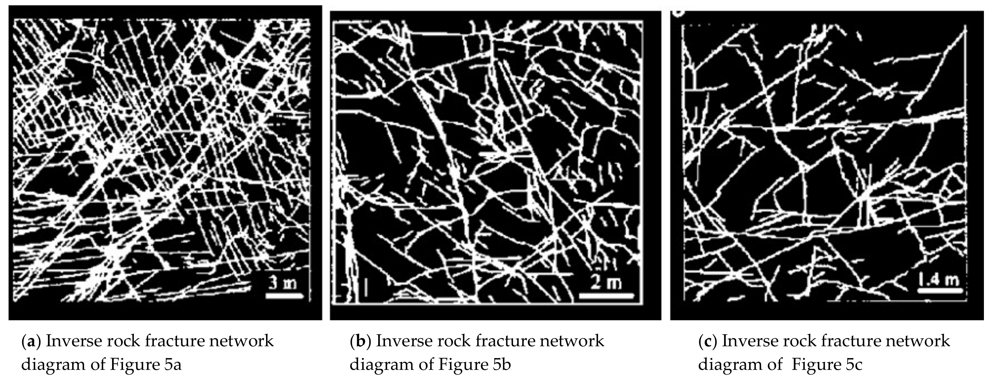
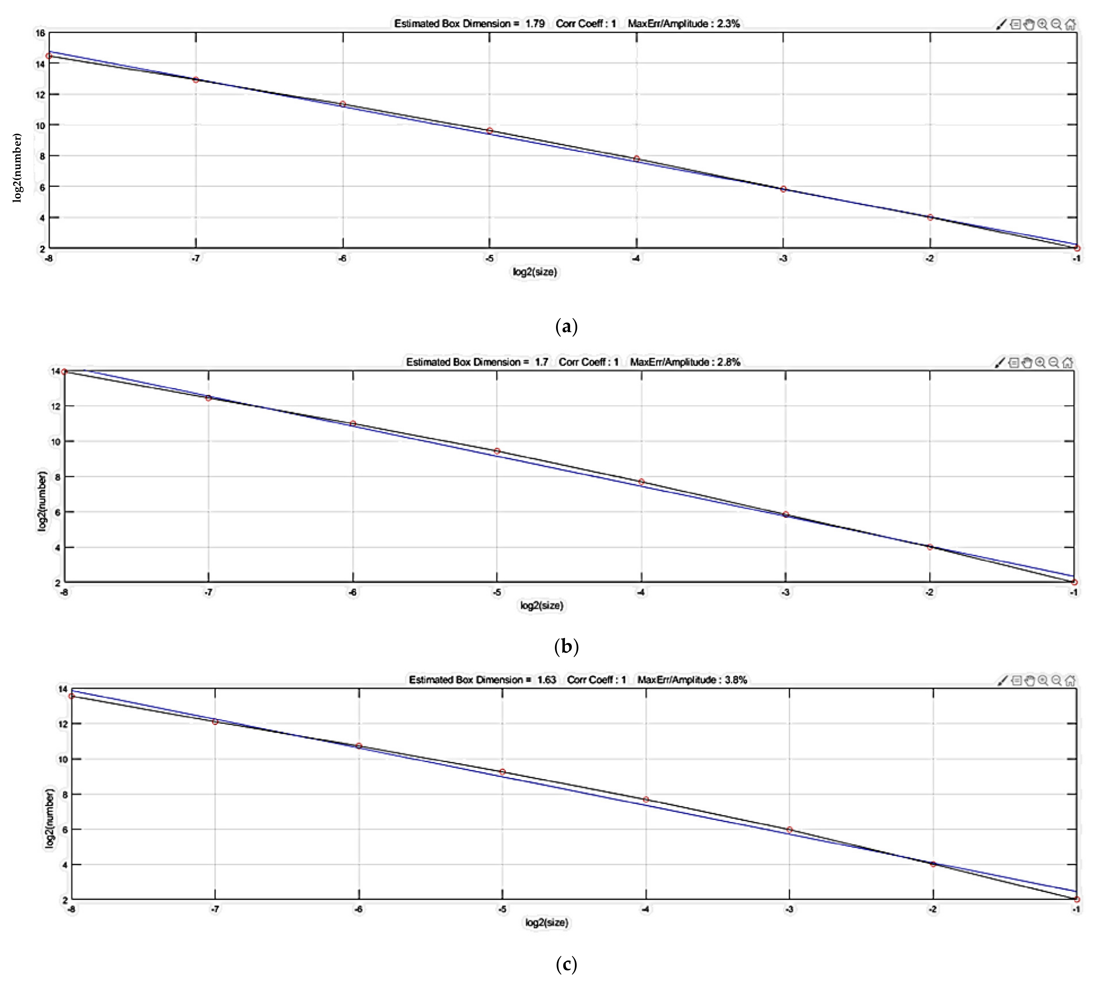
Through the calculation and analysis of three rock fracture network diagrams, the results of the simple fractal calculation method were found to be in the same order as the box-counting dimension results and the complexity of the rock fractures. This proves the effectiveness and accuracy of the fractal dimension calculation method.
(4)
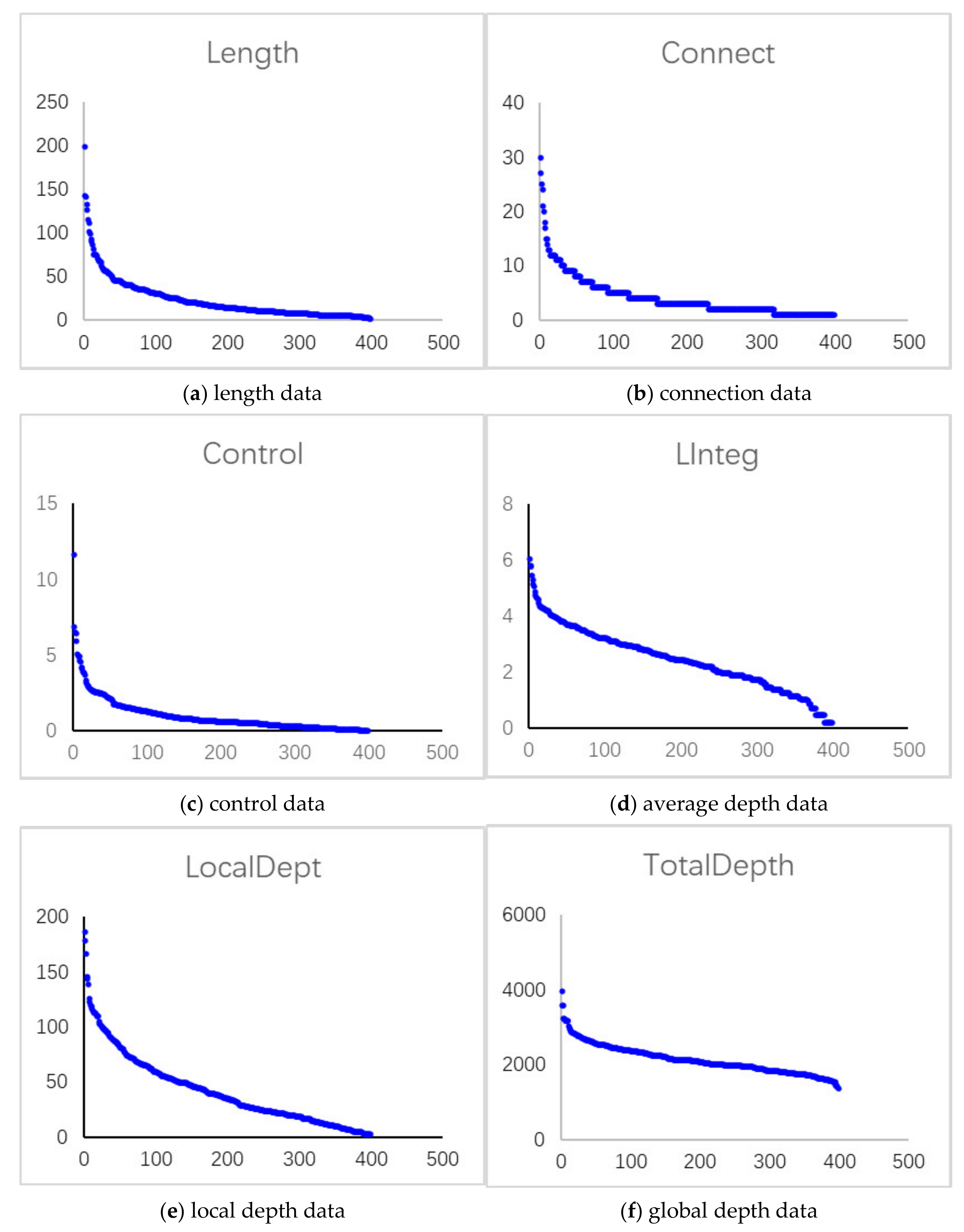
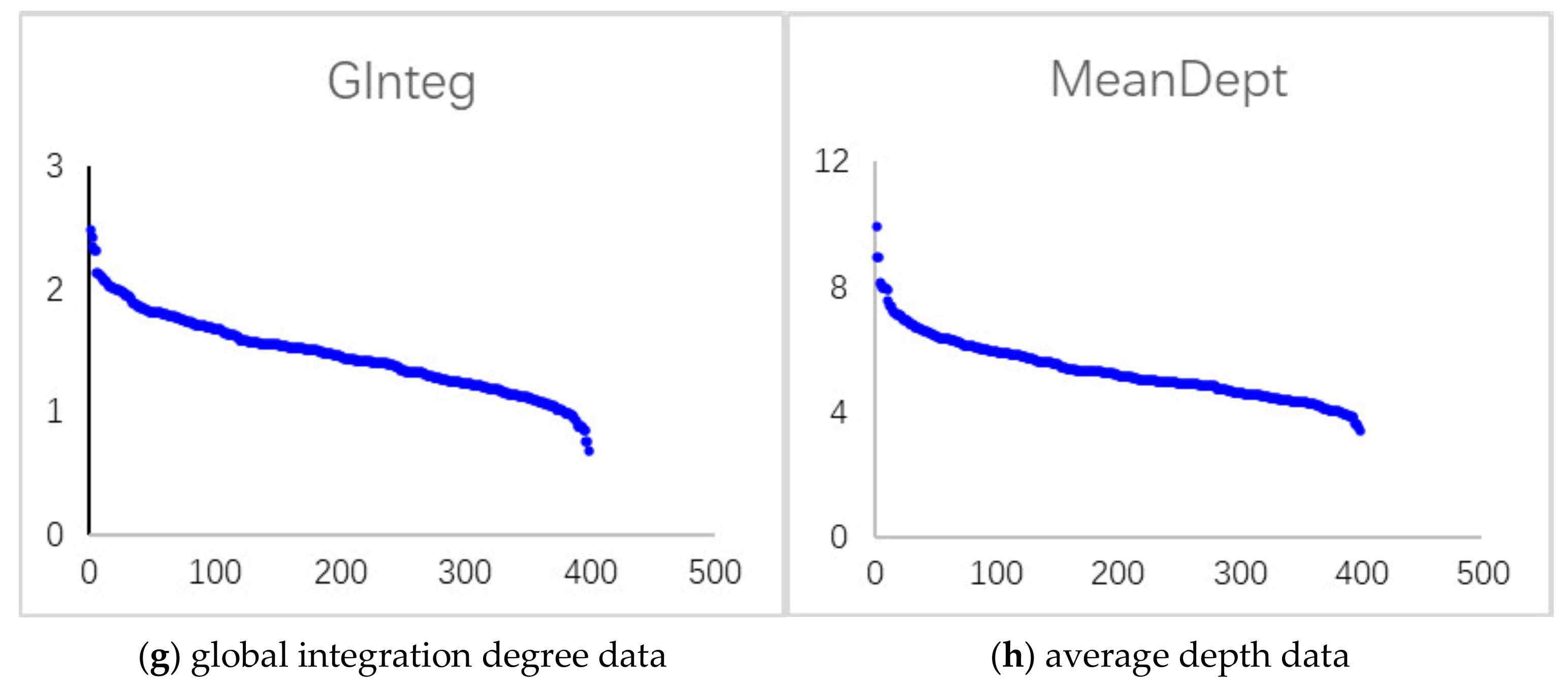
The new quantification method was used to calculate the degrees of seven space syntax metrics. It was found that there were only two kinds of heavy-tailed distributions which meet the requirements of fractals—i.e., connection value and control value. By comparing the fractal dimension with the length fractal dimension, it was found that the trend of the length fractal dimension was the same as that of the control value fractal dimension, while the fractal dimension of the connection value was contrary to it. Compared with using the length fractal dimension as a parameter, it was also found that using the connection and control data as parameters to calculate the fractal dimension could better reflect the spatial characteristics of rock fracture networks. This also proves that space syntax has certain applicability in rock fracture networks.
Because there are many calculation methods in fractal geometry, the calculation results of different rock reservoirs are different in the actual application process. Sometimes the calculation results of rock fractures with different depths, but still in the same area, will also differ. As such, the fractal dimension calculation method proposed in this paper could be a good choice for capturing the fractal characteristics of the studied objects. In addition, for the space syntax of rock fracture networks, this paper only extracted a few parameters to calculate the fractal dimensions. For research on the application of space syntax metrics in urban road traffic networks, its deep applicability in rock fracture network quantification still needs to be further explored.

Author Contributions

Conceptualization, L.S.; data curation, H.W.; methodology, J.W.; project administration, J.Z.; visualization, J.Y.; writing—review and editing, X.M.; validation, Q.S. All authors have read and agreed to the published version of the manuscript.

Funding

We gratefully acknowledge the financial support from the National Natural Science Foundation of China (11702094), China Coal Industry Association Science and Technology Research Guidance project (MTKJ2017-310), and the Key Research Program of Hebei Province (19270318D).

Data Availability Statement

Not applicable.

Conflicts of Interest

The authors declare no conflict of interest.

References

  1. Rahm, D. Regulating hydraulic fracturing in shale gas plays: The case of Texas. Energy Policy 2011, 39, 2974–2981. [Google Scholar] [CrossRef]
  2. Mark, Y.; Playton, S.; Paul, T.; Wayne, N.; Mike, S.; Robert, M. Petrophysical Challenges in Giant Carbonate Tengiz Field, Republic of Kazakhstan. Petrophysics 2015, 56, 615–647. [Google Scholar]
  3. Hu, X.; Yu, W.; Liu, M.; Wang, M.; Wang, W. A multiscale model for methane transport mechanisms in shale gas reservoirs. J. Pet. Sci. Eng. 2019, 172, 40–49. [Google Scholar] [CrossRef]
  4. Bonnet, E.; Bour, O.; Odling, N.E.; Davy, P.; Main, I.G.; Cowie, P.; Berkowitz, B. Scaling of fracture systems in geological media. Rev. Geophys. 2001, 39, 347–383. [Google Scholar] [CrossRef] [Green Version]
  5. Hobé, A.; Vogler, D.; Seybold, M.P.; Ebigbo, A.; Settgast, R.R.; Saar, M.O. Estimating fluid flow rates through fracture networks using combinatorial optimization. Adv. Water Resour. 2018, 122, 85–97. [Google Scholar] [CrossRef] [Green Version]
  6. Figueroa Pilz, F.; Dowey, P.J.; Fauchille, A.L.; Courtois, L.; Bay, B.; Ma, L.; Taylor, K.; Meckleburgh, J.; Lee, P. Synchrotron tomographic quantification of strain and fracture during simulated thermal maturation of an organic-rich shale, UK Kimmeridge Clay. J. Geophys. Res. Solid Earth 2017, 122, 2553–2564. [Google Scholar] [CrossRef] [Green Version]
  7. Le, T.D.; Murad, M.A. A new multiscale model for flow and transport in unconventional shale oil reservoirs. Appl. Math. Model. 2018, 64, 453–479. [Google Scholar] [CrossRef]
  8. Li, X.; Zuo, Y.; Zhuang, X.; Zhu, H. Estimation of fracture trace length distributions using probability weighted moments and L-moments. Eng. Geol. 2014, 168, 69–85. [Google Scholar] [CrossRef]
  9. Lu, J.; Ghassemi, A. Estimating natural fracture orientations using geomechanics based stochastic analysis of microseismicity related to reservoir stimulation. Geothermics 2019, 79, 129–139. [Google Scholar] [CrossRef]
  10. Kevin Bisdom, G.B.; Hamidreza, M.N. The impact of different aperture distribution models and critical stress criteria on equivalent permeability in fractured rocks. J. Geophys. Res. Solid Earth 2015, 10, 1002. [Google Scholar]
  11. El-Emam, H.; Elsisi, A.; Salim, H.; Sallam, H. Fatigue Crack Tip Plasticity for Inclined Cracks. Int. J. Steel Struct. 2018, 18, 443–455. [Google Scholar] [CrossRef]
  12. Roy, A.; Perfect, E.; Dunne, W.M.; McKay, L.D. A technique for revealing scale-dependent patterns in fracture spacing data. J. Geophys. Res. Solid Earth 2014, 119, 5979–5986. [Google Scholar] [CrossRef]
  13. Babanouri, N.; Nasab, S.K.; Sarafrazi, S. A hybrid particle swarm optimization and multi-layer perceptron algorithm for bivariate fractal analysis of rock fractures roughness. Int. J. Rock Mech. Min. Sci. 2013, 60, 66–74. [Google Scholar] [CrossRef]
  14. Geng, L.; Li, G.; Wang, M.; Li, Y.; Tian, S.; Pang, W.; Lyu, Z. A fractal production prediction model for shale gas reservoirs. J. Nat. Gas Sci. Eng. 2018, 55, 354–367. [Google Scholar] [CrossRef]
  15. Riley, P.; Tikoff, B.; Murray, A.B. Quantification of fracture networks in non-layered, massive rock using synthetic and natural data sets. Tectonophysics 2011, 505, 44–56. [Google Scholar] [CrossRef]
  16. Miao, T.; Yu, B.; Duan, Y.; Fang, Q. A fractal analysis of permeability for fractured rocks. Int. J. Heat Mass Transf. 2015, 81, 75–80. [Google Scholar] [CrossRef]
  17. Huang, S.; Yao, Y.; Zhang, S.; Ji, J.; Ma, R. Pressure transient analysis of multi-fractured horizontal wells in tight oil reservoirs with consideration of stress sensitivity. Arab. J. Geosci. 2018, 11, 285. [Google Scholar] [CrossRef]
  18. Wang, L.; Duan, K.; Zhang, Q.; Li, X.; Jiang, R. Study of the Dynamic Fracturing Process and Stress Shadowing Effect in Granite Sample with Two Holes Based on SCDA Fracturing Method. Rock Mech. Rock Eng. 2022, 55, 1537–1553. [Google Scholar] [CrossRef]
  19. Silberschmidt, V.V.; Silberschmidt, V.G. Fractal models in rock fracture analysis. Terra Nova 2010, 2, 483–488. [Google Scholar] [CrossRef]
  20. Koike, K.; Kaneko, K. Characterization and modeling of fracture distribution in rock mass using fractal theory. Geotherm. Sci. Technol. 1999, 6, 43–62. [Google Scholar]
  21. Zhou, Z.; Su, Y.; Wang, W.; Yan, Y. Integration of microseismic and well production data for fracture network calibration with an L-system and rate transient analysis. J. Unconv. Oil Gas Resour. 2016, 15, 113–121. [Google Scholar] [CrossRef]
  22. Liu, G.; Yu, B.; Ye, D.; Gao, F.; Liu, J. Study on Evolution of Fractal Dimension for Fractured Coal Seam under Multi-Field Cou-pling. Fractals 2020, 28, 2050072. [Google Scholar] [CrossRef]
  23. Mecholsky, J.J.; Passoja, D.E.; Feinberg-Ringel, K.S. Quantitative Analysis of Brittle Fracture Surfaces Using Fractal Geometry. J. Am. Ceram. Soc. 2010, 72, 1–12. [Google Scholar] [CrossRef]
  24. Sheng, G.; Su, Y.; Wang, W.; Javadpour, F.; Tang, M. Application of Fractal Geometry in Evaluation of Effective Stimulated Reser-voir Volume in Shale Gas Reservoirs. Fractals 2017, 25, 1740007. [Google Scholar] [CrossRef] [Green Version]
  25. Sui, L.; Ju, Y.; Yang, Y.; Yang, Y.; Li, A. A quantification method for shale fracability based on analytic hierarchy process. Energy 2016, 115, 637–645. [Google Scholar] [CrossRef]
  26. Gillespie, P.A.; Walsh, J. Measurement and characterisation of fractures of space distributions. Tectonophysics 1993, 226, 113–141. [Google Scholar] [CrossRef]
  27. Walsh, J.; Watterson, J. Fractal analysis of fracture patterns using the standard box-counting technique: Valid and invalid methodologies. J. Struct. Geol. 1993, 15, 1509–1512. [Google Scholar] [CrossRef]
  28. Jafari, A.; Babadagli, T. Estimation of equivalent fracture network permeability using fractal and statistical network properties. J. Pet. Sci. Eng. 2012, 92–93, 110–123. [Google Scholar] [CrossRef]
  29. Space Syntax Network. Available online: https://www.spacesyntax.net/ (accessed on 17 January 2021).
  30. UCL. Space Syntax: Overview. Available online: https://www.spacesyntax.online/overview-2/ (accessed on 17 January 2021).
  31. Hillier, B.H.J. The Social Logic of Space; Cambridge University Press: Cambridge, UK, 1984. [Google Scholar]
  32. Thomson, R.C. Bending the axial line smoothly continuous road centre-line segments as a basis for road network analysis. In Proceedings of the 4th International Space Syntax Symposium, London, UK, 17–19 June 2003. [Google Scholar]
  33. Liu, X.; Jiang, B. Defining and generating axial lines from street center lines for better understanding of urban morphologies. Int. J. Geogr. Inf. Sci. 2012, 26, 1521–1532. [Google Scholar] [CrossRef]
  34. Jiang, B.; Claramunt, C. Topological Analysis of Urban Street Networks. Environ. Plan. B Plan. Des. 2004, 31, 151–162. [Google Scholar] [CrossRef] [Green Version]
  35. Jiang, B.; Zhao, S.; Yin, J. Self-organized natural roads for predicting traffic flow: A sensitivity study. J. Stat. Mech. Theory Exp. 2008, 2008, P07008. [Google Scholar] [CrossRef] [Green Version]
  36. Jeong, S.-K.; Ban, Y.-U. Developing a topological information extraction model for space syntax analysis. Build. Environ. 2011, 46, 2442–2453. [Google Scholar] [CrossRef]
  37. Jiang, B.; Liu, C. Street-based topological representations and analyses for predicting traffic flow in GIS. Int. J. Geogr. Inf. Sci. 2009, 23, 1119–1137. [Google Scholar] [CrossRef] [Green Version]
  38. Mustafa, F.A.; Rafeeq, D.A. Assessment of elementary school buildings in Erbil city using space syntax analysis and school teachers′ feedback. Alex. Eng. J. 2019, 58, 1039–1052. [Google Scholar] [CrossRef]
  39. Xu, P.; Yu, B.; Qiu, S.; Cai, J. An analysis of the radial flow in the heterogeneous porous media based on fractal and constructal tree networks. Phys. A Stat. Mech. Its Appl. 2008, 387, 6471–6483. [Google Scholar] [CrossRef]
  40. Zheng, Q.; Yu, B.; Wang, S.; Luo, L. A diffusivity model for gas diffusion through fractal porous media. Chem. Eng. Sci. 2012, 68, 650–655. [Google Scholar] [CrossRef]
  41. Shen, Y.; Xu, P.; Qiu, S.; Rao, B.; Yu, B. A generalized thermal conductivity model for unsaturated porous media with fractal ge-ometry. Int. J. Heat Mass Transf. 2020, 152, 119540. [Google Scholar] [CrossRef]
  42. Boming, Y.; Cheng, P. A fractal permeability model for bi-dispersed porous media. Int. J. Heat Mass Transf. 2002, 45, 2983–2993. [Google Scholar]
  43. Xu, P.; Yu, B. Developing a new form of permeability and Kozeny–Carman constant for homogeneous porous media by means of fractal geometry. Adv. Water Resour. 2008, 31, 74–81. [Google Scholar] [CrossRef]
  44. Miao, T.; Chen, A.; Zhang, L.; Yu, B. A novel fractal model for permeability of damaged tree-like branching networks. Int. J. Heat Mass Transf. 2018, 127, 278–285. [Google Scholar] [CrossRef]
  45. Sui, L.; Yu, J.; Cang, D.; Miao, W.; Wang, H.; Zhang, J.; Yin, S.; Chang, K. The fractal description model of rock fracture networks characterization. Chaos Solitons Fractals 2019, 129, 71–76. [Google Scholar] [CrossRef]
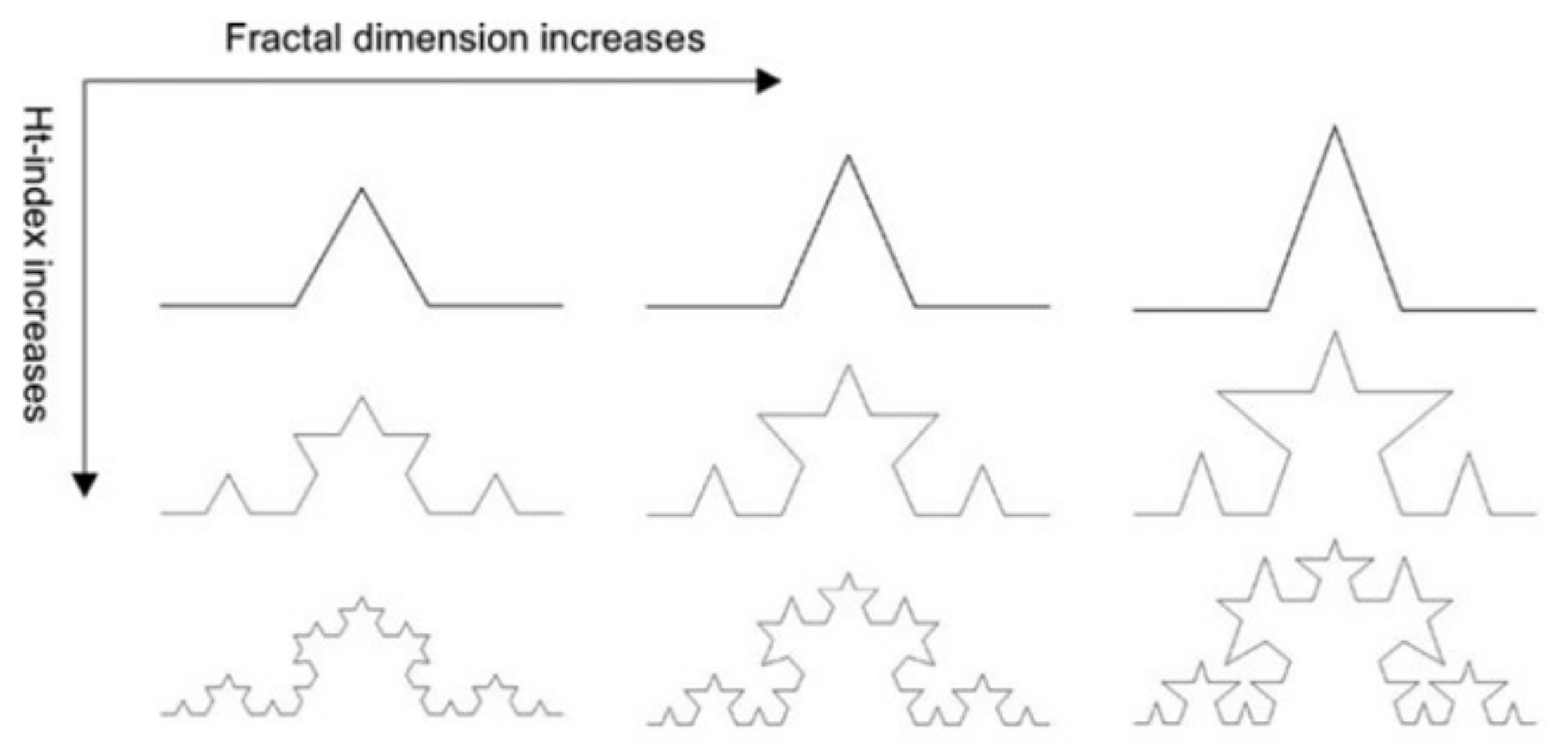
  46. Ding, M.; Jiang, B. A Smooth Curve as a Fractal under the Third Definition. Cartographica 2018, 53, 203–210. [Google Scholar]
  47. Jiang, B. Head/Tail Breaks: A New Classification Scheme for Data with a Heavy-Tailed Distribution. Prof. Geogr. 2013, 65, 482–494. [Google Scholar] [CrossRef]
  48. Jiang, B.; Yin, J. Ht-Index for Quantifying the Fractal or Scaling Structure of Geographic Features. Ann. Assoc. Am. Geogr. 2013, 104, 530–540. [Google Scholar] [CrossRef]
  49. Chelidze, T.; Gueguen, Y. Evidence of fractal fracture. Int. J. Rock Mech. Ming Sci. Geome-Chanics Abstr. 1990, 27, 223–225. [Google Scholar] [CrossRef]
  50. Jiang, B. A Recursive Definition of Goodness of Space for Bridging the Concepts of Space and Place for Sustainability. Sustainability 2019, 11, 4091. [Google Scholar] [CrossRef] [Green Version]
  51. Jiang, B. Living Structure Down to Earth and Up to Heaven: Christopher Alexander. Urban Sci. 2019, 3, 96. [Google Scholar] [CrossRef] [Green Version]
Figure 1. Koch curve.
Fractalfract 06 00353 g001
Figure 2. Inverse Koch curve.
Fractalfract 06 00353 g002
Figure 3. Calculation results of the box-counting dimension of the Koch curve.
Fractalfract 06 00353 g003
Figure 4. HT index and fractal dimension characterizing the cubic iterative Koch curve (Reprinted from Figure 8 of reference [48]. Ht-Index for Quantifying the Fractal or Scaling Structure of Geographic Features, Bin Jiang and Junjun Yin, Annals of the Association of American Geographers, copyright © 2014 The Association of American Geographers, reprinted by permission of Taylor & Francis Ltd. (Abingdon, UK), http://www.tandfonline.com (accessed on 6 April 2022) on behalf of The Association of American Geographers, www.aag.org (accessed on 6 April 2022)).
Fractalfract 06 00353 g004
Figure 5. Three rock fracture network diagrams (Reprinted from Figure 11 of reference [28]. Journal of Petroleum Science and Engineering, 92, Alireza Jafari and Tayfun Babadagli, Estimation of equivalent fracture network permeability using fractal and statistical network properties, 110–123, Copyright (2012), with permission from Elsevier (Amsterdam, The Netherlands)).
Fractalfract 06 00353 g005
Figure 6. The three inverse rock fracture network diagrams of Figure 5.
Fractalfract 06 00353 g006
Figure 7. Calculation results of the box-counting dimension of the three rock fracture network diagrams (ac).
Fractalfract 06 00353 g007
Figure 8. Power law analysis of metric and length of space syntax in (Figure 5 fracture network diagrams (c)) (the horizontal axis data represent the fracture ID, and the vertical axis data are the dimensionless data of these 8 parameters).
Fractalfract 06 00353 g008aFractalfract 06 00353 g008b
Table 1. Head/tail break data from Figure 5 (where N is the number, M is the average, Hi (i = 1,2,3,4,5) is the head of the ith breaking, and Ti (i = 1,2,3,4,5) is the tail of the ith breaking).
Figure 5aFigure 5bFigure 5c
NMNMNM
Total414.0022.64261.0019.49139.0028.09
H1138.0047.2594.0038.1547.0057.19
T1276.0010.34167.008.9892.0013.23
H1 (%)0.33 0.36 0.34
T1 (%)0.67 0.64 0.66
H240.0080.0028.0065.2117.0088.18
T298.0033.8866.0026.6730.0039.63
H2 (%)0.29 0.30 0.36
T2 (%)0.71 0.70 0.64
H313.00117.159.0097.227.00120.29
T327.0062.1119.0050.0510.0065.70
H3 (%)0.33 0.32 0.41
T3 (%)0.68 0.68 0.59
H45.00148.603.00137.003.00147.00
T48.0097.506.0077.334.00100.25
H4 (%)0.38 0.33 0.43
T4 (%)0.62 0.67 0.57
H51.00199.001.00159.001.00183.00
T54.00136.002.00126.002.00129.00
H5 (%)0.20 0.33 0.33
T5 (%)0.80 0.67 0.67
Table 2. Figure 5c space syntax metric and length HT index.
ConnectControlMeanDeptGIntegLIntegTotalDepthLocalDeptLength
HT Index46111116
Publisher’s Note: MDPI stays neutral with regard to jurisdictional claims in published maps and institutional affiliations.

