1. Introduction
Fractional calculus has resurged in popularity throughout the last couple of decades. We must acknowledge that novel notions and tactics arise inside the domain underlying fractional calculus. Then, newly difficult findings and startling linkages between distinct disciplines of physics might be obtained. Nonlinear partial differential equations (NPDEs) [
1,
2,
3] are utilized to represent actual systems in several scientific disciplines. Furthermore, even though they characterize many physical systems, a few of them seem to be not necessarily solvable. It is demonstrated that, for the genuine models represented by NPDEs, several events that are frequently unknown or overlooked pique the interest of researchers in the field. From a mathematical standpoint, using sophisticated methods to generate structures for a framework underlying dynamic defined by an NPDE should represent an important goal. Likewise, the non-integer order derivative is more precise and efficient in simulating significant issues, which is especially evident in a framework in which memory or genetic property features take part in crucial importance or are emphasized. In this regard, it is demonstrated that fractional calculus offers the benefit of assisting in the accurate modeling of natural processes [
4,
5].
Investigating a family of temporal time-FNEE models, including time-FCDs, is essential in many nonlinear wave dispersion situations. Additionally, to do this, a highly accurate semi-analytical technique is created as well as constructed with the residual error factors in mind toward addressing a category of fifth-order time FCKdVEs [
6]. This work [
7] investigates the dynamical activity with its dispersive extended nonlinear Schrödinger equation (NLSE). Non-linearity, as well as wave speed impacts on wave outlines, was also investigated [
8,
9].
Recent research has illustrated that many physical occurrences can be interpreted as non-conservative. Consequently, to improve prior integer order frameworks and gain a deeper knowledge of irregular dynamics, fractional calculus should be employed to represent nonlinear complicated physical processes [
10]. The non-locality behavior demonstrates a significant divergence among FO differential operators and integer-order differential operators. This property makes FO models increasingly appealing to researchers, even though FO structures are more genuine and useful than traditional integer-order models. Indeed, whenever the FO value is set to 1, the FO model equations automatically translate to integer-order counterparts. As a result, fractional calculus arises as a fresh study axis in various scientific areas. In reality, fractional calculus has been employed in a variety of domains (oceanography, atmospheric research, colored noise, solid mechanics, physical phenomenon modeling, finance, and economics) [
10]. Similarly, addressing time-fractional model equations seems to be a critical research focus. There are several ways for determining the solutions of time-fractional equations (variational–iteration method,
-expansion method, tanh–coth method,
-expansion method, expansion method, and so forth).
Nonlinear differential equations are frequently utilized to evaluate complex scientific phenomena, including optics, deeper water, quantum mechanics, biophysics, fluid mechanics, plasma physics, marine engineering, chemistry, and physics. Furthermore, more and more amazing approaches of discovering new exact and explicit solutions for NPDEs is cited in the literature as [
11].
A soliton, also known as a solitary wave, is a wave whose propagation speed is independent of its amplitude. Solitons are commonly seen in fluid mechanics. These are waves that interact in a nonlinear way. Nonlinear interaction produces solitonic waves that keep their structure and amplitude. The soliton hypothesis has sparked active research in a variety of scientific domains all around the world. Solitons are now widely accepted as the product of an equilibrium between weak nonlinearity and dispersion. Due to its importance in several scientific domains, such as fluid dynamics, astrophysics, plasma physics, and magneto-acoustic waves, among others, the soliton idea has drawn a large number of investigations. The multi-dimensional Boiti–Leon–Manna–Pempinelli equations’ optical soliton solutions are calculated in the research article [
12].
The idea of optical solitons is remarkable, as soliton solutions can be found in a variety of mathematical physics model equations. Viewing optical solitons is one of the most important aspects of nonlinear fiber optics. In applied science and engineering, the soliton has a number of uses. Nonlinear differential equations can be solved using a variety of strategies. This new expanded direct algebraic method [
13] is one such example. M.B. Riaz investigated the exact solutions for blood flow through a circular tube under magnetic field influence using Caputo–Fabrizio FO derivatives [
14] and synchronization for the tumor-immune framework using FO [
15], as well as a systematic investigation to discover and analyze the knowledge to decide the truth. In the creation of solving models of executions, fractional calculus has made tremendous progress, and it strives to demonstrate that it can generate a more accurate model [
16,
17].
Nonetheless, not all suggested or recognized NPDEs or non-integer order nonlinear partial differential equations (NPDEs) can indeed be addressed using a variety of approaches [
18,
19]. The non-integer order partial differential equation under consideration drives the voltage dynamics of such a fractional discrete nonlinear electrical transmitting lattice. This framework is a good illustration of a system that may assist readers in analyzing the behavior of nonlinear excitation passing through a nonlinear electrical transmission channel as well as related waveguides [
20]. The contribution of our article is twofold: first, to build an intrinsic non-integer order discrete nonlinear electrical transmission lines (FDNETL) [
21,
22], and second, to obtain new results in terms of exact soliton solutions since employing some impactful methods, such as the fractional complex transform as well as modified Riemann–Liouville (mRL) derivatives.
The hereunder is the paper’s arrangement:
Section 2 is dedicated to displaying an overview of the non-integer order complex transform and the method, along with an outline of the non-integer order complex transform and recapitulation for the generalized auxiliary equation method. In
Section 3, there is the model’s mathematical portrayal.
Section 4 deals with the examination of the analytical solutions.
Section 5 displays the results in a graphical layout. Furthermore, there is a detailed physical interpretation of results with deliberation to easily understand the effective exploit of solitary wave solutions. The sensitivity assessment and quasi-periodic behaviors are reported in
Section 6. The conclusion is included in
Section 7.
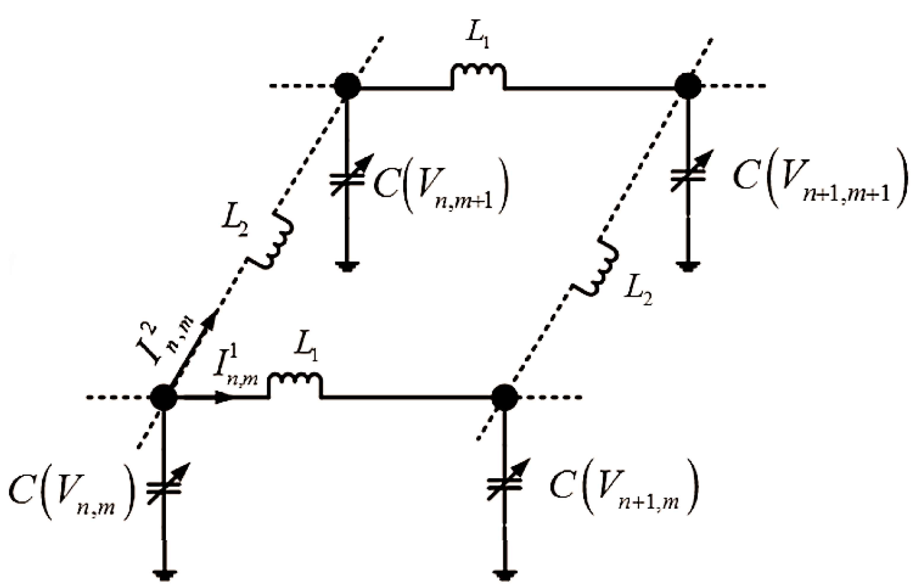
3. The Model’s Mathematical Portrayal
We employ a model built by connecting 1D nonlinear electrical transmission lines (NETL) in a lattice by a capacitor with a constant capacitance
in the transverse direction. A fractional capacitor, such as two nodes separated by an inductor, is used to assemble the 1D NETL periodically [
21,
26,
27].
Curie’s 1889 empirical law dictates the current flowing through the fractional nonlinear capacitor at [
21]. Westerlund confirmed this empirically.
refers to the capacitor’s losses.
Figure 1 depicts the series branch of a constant inductor
L routed via a fractional nonlinear capacitor. Because of the inductor’s proximity effect as well as the capacitor’s inefficiencies, we record the voltage as
from
Figure 1,
represents the voltage on the node
, while
n signifies the horizontal line but also
m indicates the wave’s transverse propagative direction [
28]. However, in Kirchhoff’s equation, solitons are used in a variety of ways. The Kirchhoff wave equation is expressed in terms of classical field theory. This allows examining the presence of soliton solutions by introducing the spontaneous symmetry breaking phenomena into the study of linear structures, such as strings. In [
29], in the space of the spatial gradient of the lateral displacement of a string, they discovered
solitons. This aids in the detection of stable states in string deformations. In [
30], the researchers investigated the presence of several soliton solutions on Kirchhoff-type issues affecting critical progression in this paper. We derive an endless number of solutions that tend to zero for acceptable positive parameters utilizing the concentration–compactness principle and mini-max approaches.
The application of Kirchhoff’s laws toward the model yields discrete fractional nonlinear PDEs:
the charge of the nonlinear capacitor is denoted by
, wherein
and
represent nonlinear coefficients that govern the amount of electric charge retained in the capacitors.
We derive by simply adopting the semi-discrete approximation for
.
Let us put Equation (
28) within Equation (
27), and by taking into account
and
such that
and
, we obtain
we construct the exact fractional solutions for the investigated model via implementing the mRL derivatives in combination with fractional complex transform [
10] and adopting
where
wherein
are random parameters. Equation (
30) is the following result:
thus, making the assumption that
, Equation (
30) yields the integration constant during twice successive integrations and is equal to zero.
5. Results in Graphical Layout
The section is dedicated to giving a graphical representation for some analytical outcomes stated across the research. Overall, the section focuses on the underlying knowledge of some of the individual results documented in this investigation. To construct graphs for clearer illustration, a current professional programming software tool is employed. In addition, each 2D, 3D, and 2D-contour plot is displayed over a distinct interval in
Figure 2,
Figure 3,
Figure 4,
Figure 5,
Figure 6,
Figure 7,
Figure 8,
Figure 9,
Figure 10,
Figure 11,
Figure 12 and
Figure 13. Contour plots are extremely useful when it is difficult to perceive physical processes in three dimensions properly. We use different colors just to make sure that the behavior of the wave is going to change or that there is the overlapping of different waves or that different curves appear in the same wave at different points, and we use contour graph to give us a better idea of where there is similarity, where the graph disappears or may become inconsistent or sometimes become discontinued.
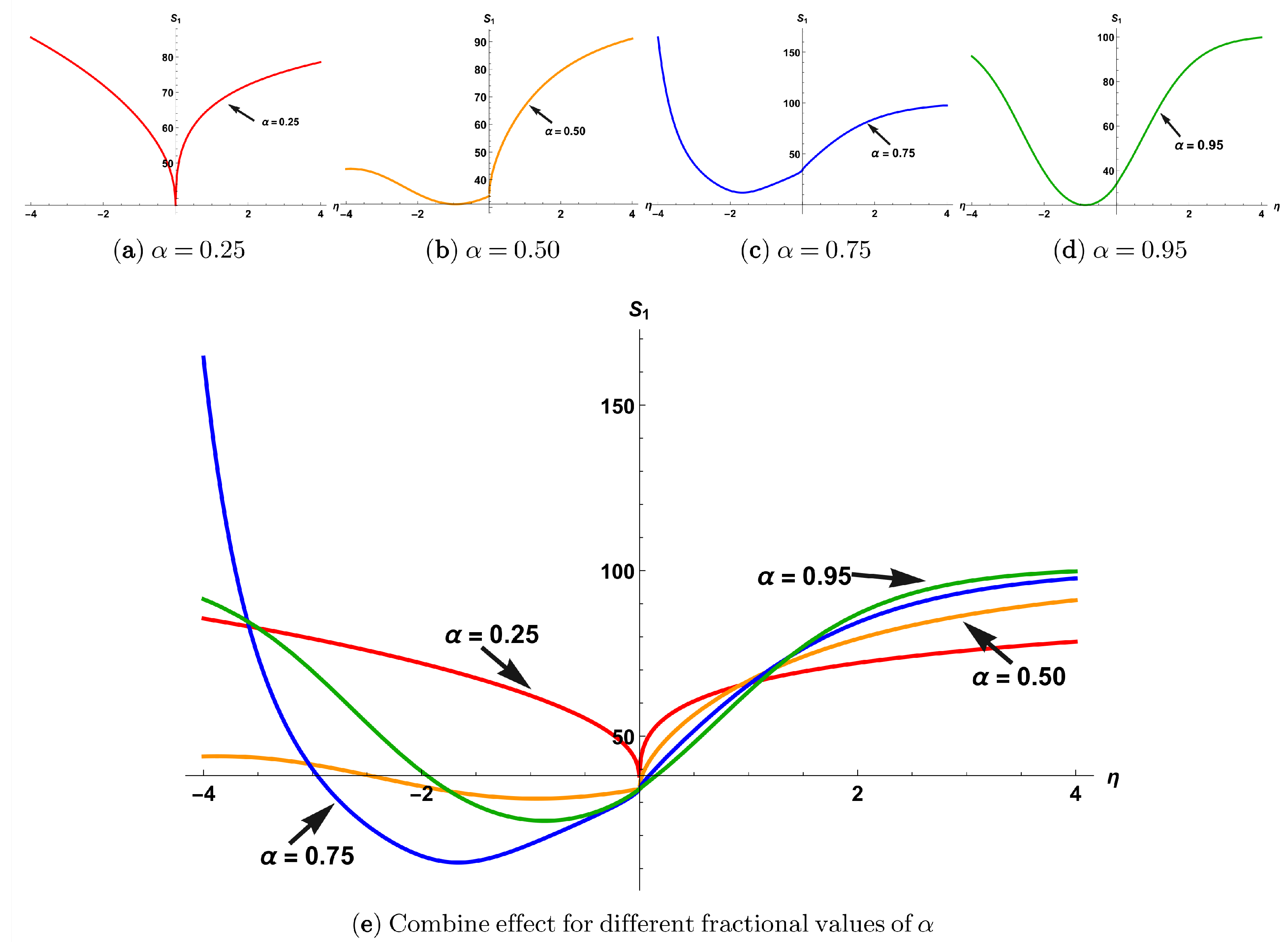
Relevant quantities for parameters can be used relying on their physical regions. We may examine unique dynamic properties, forms, and patterns of soliton solutions by using variable characteristic values as a primary component of our investigation. Yet, it is important to remember that solutions include trigonometric functions and combined hyperbolic modules, as well as rational functions.
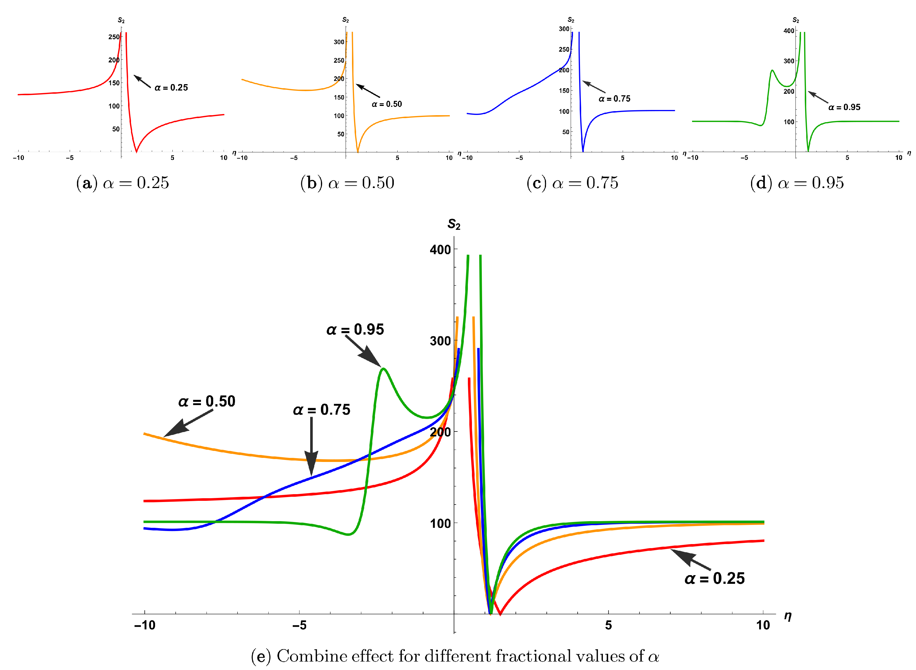
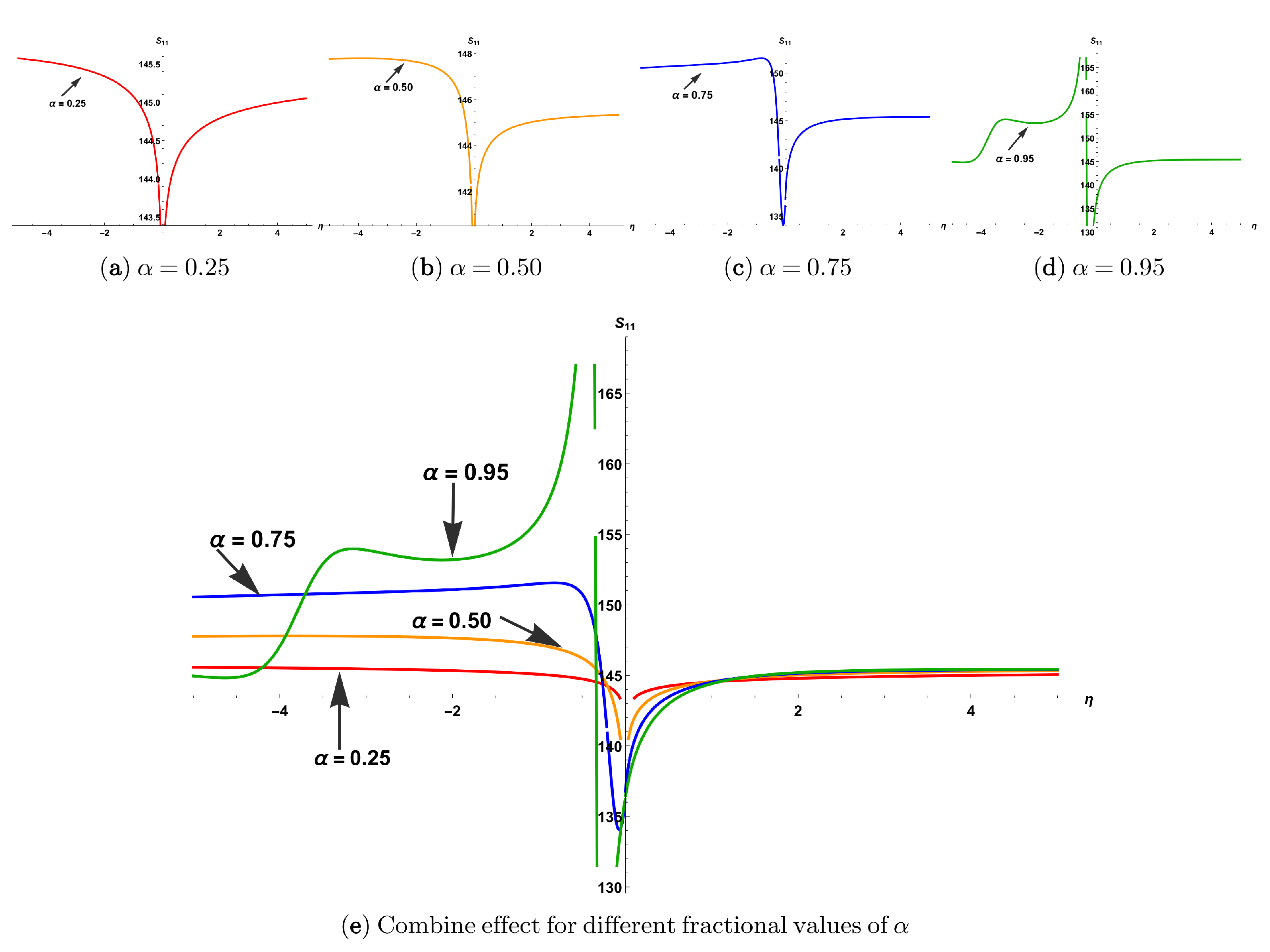
One such diagram depicts a physical understanding of . Here is a graphical representation of the examination using the parameters, , , , , , , , while (red), (yellow), (blue), and (green), within the interval
Figure 2.
A 2D graphical representation for .
Figure 2.
A 2D graphical representation for .
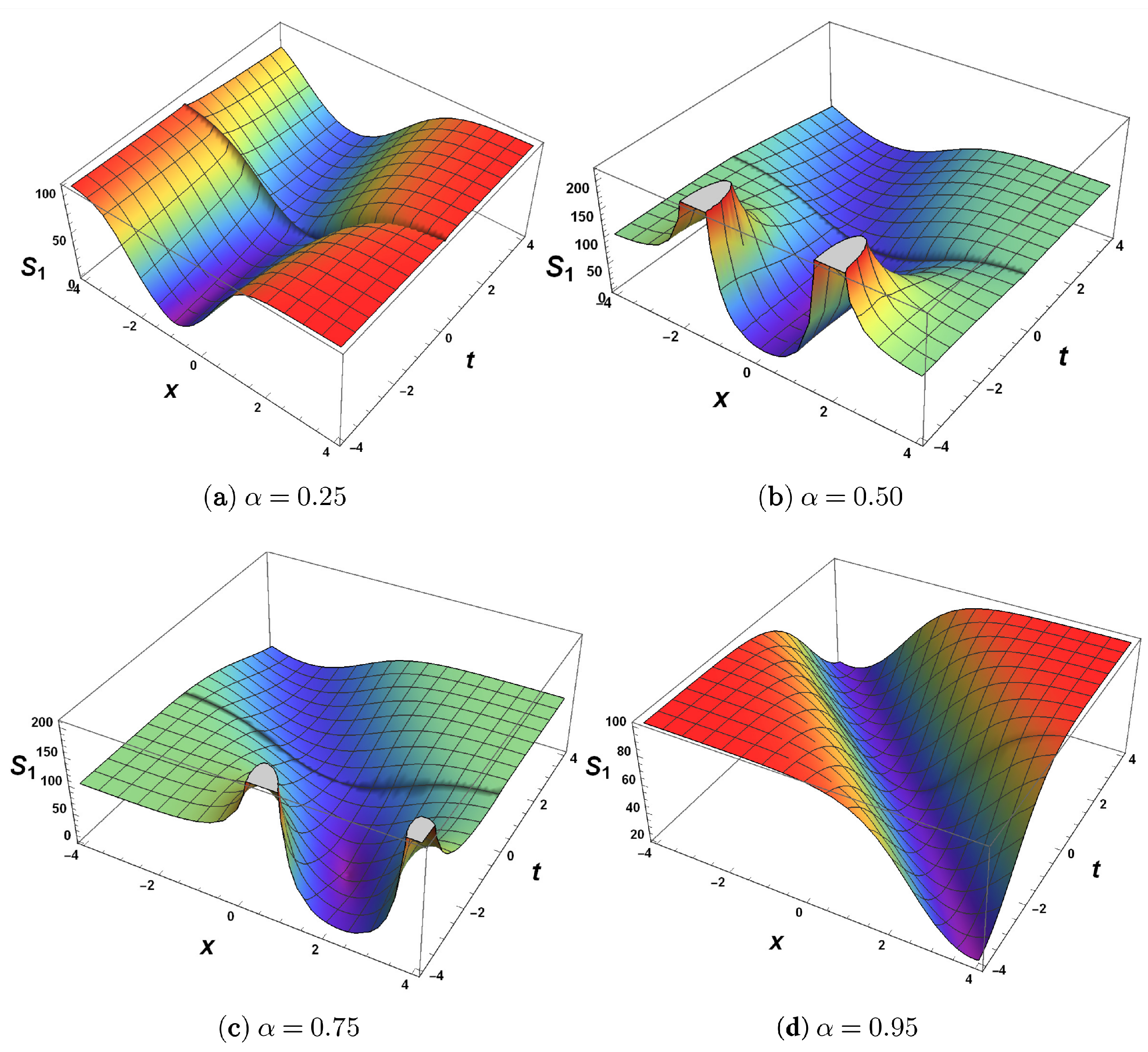
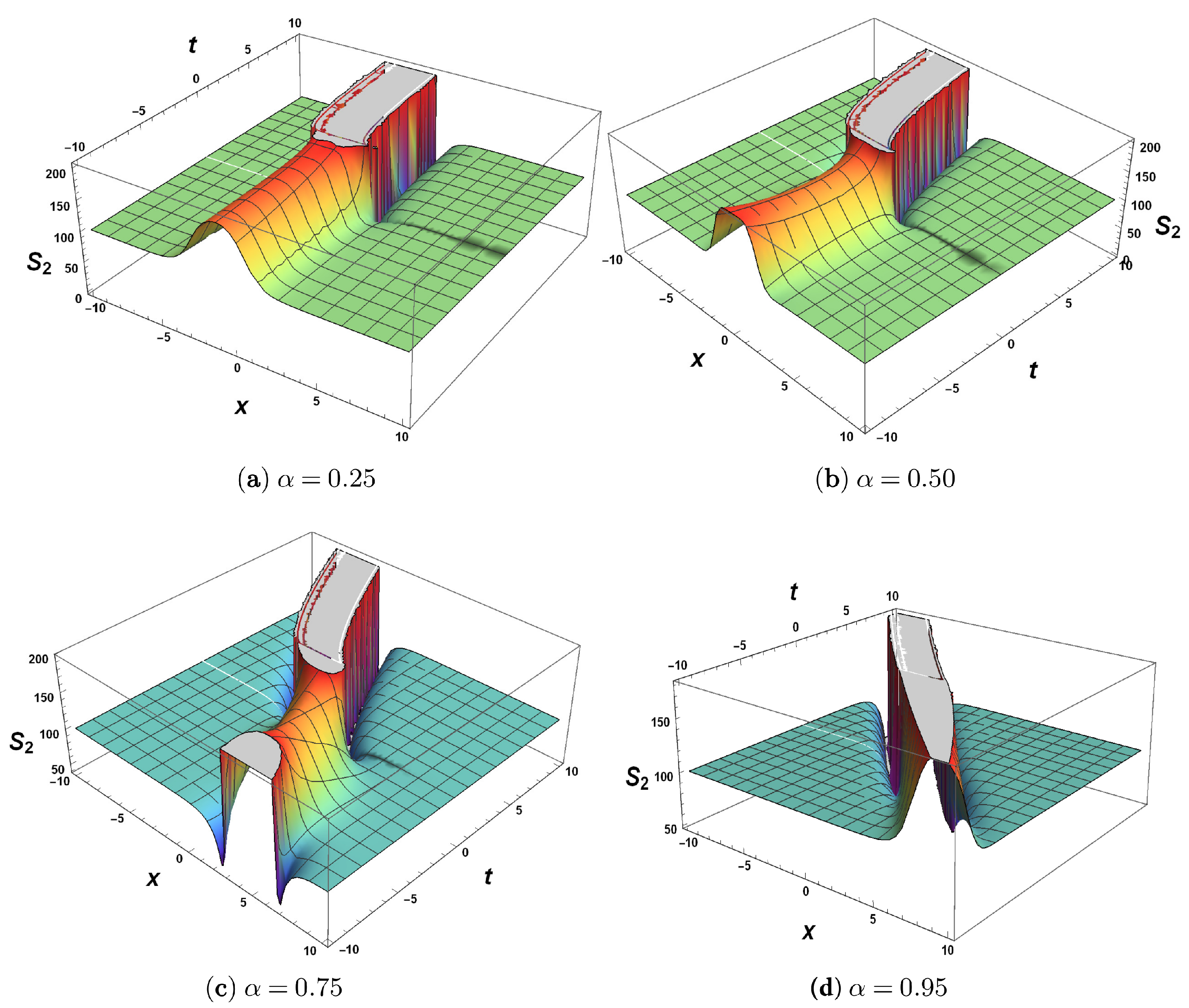
Figure 3.
A 3D graphical representation for .
Figure 3.
A 3D graphical representation for .
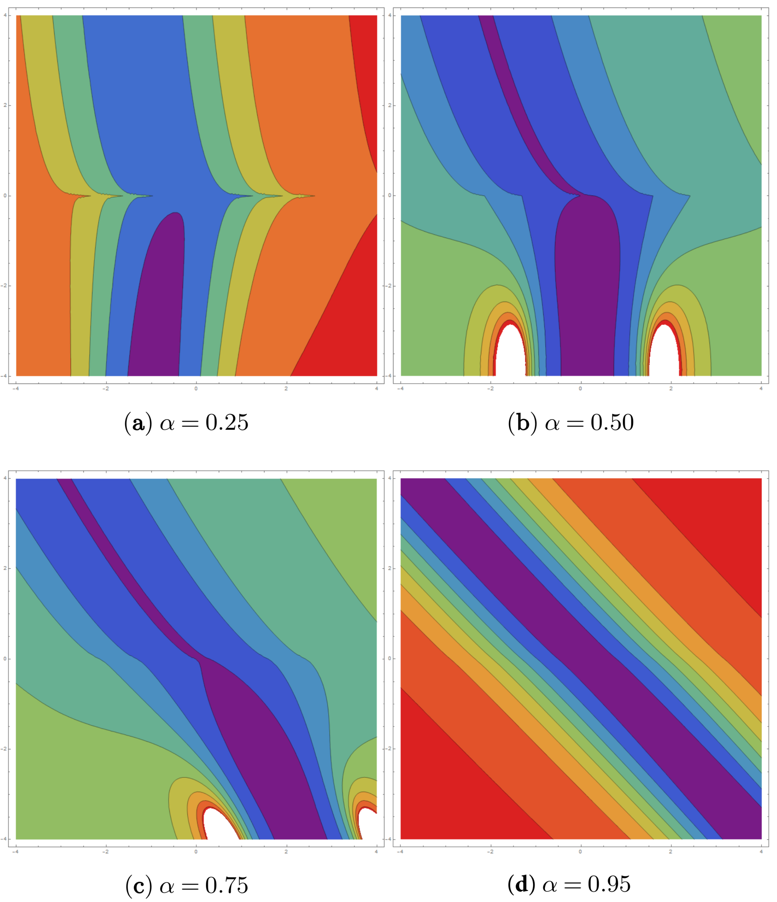
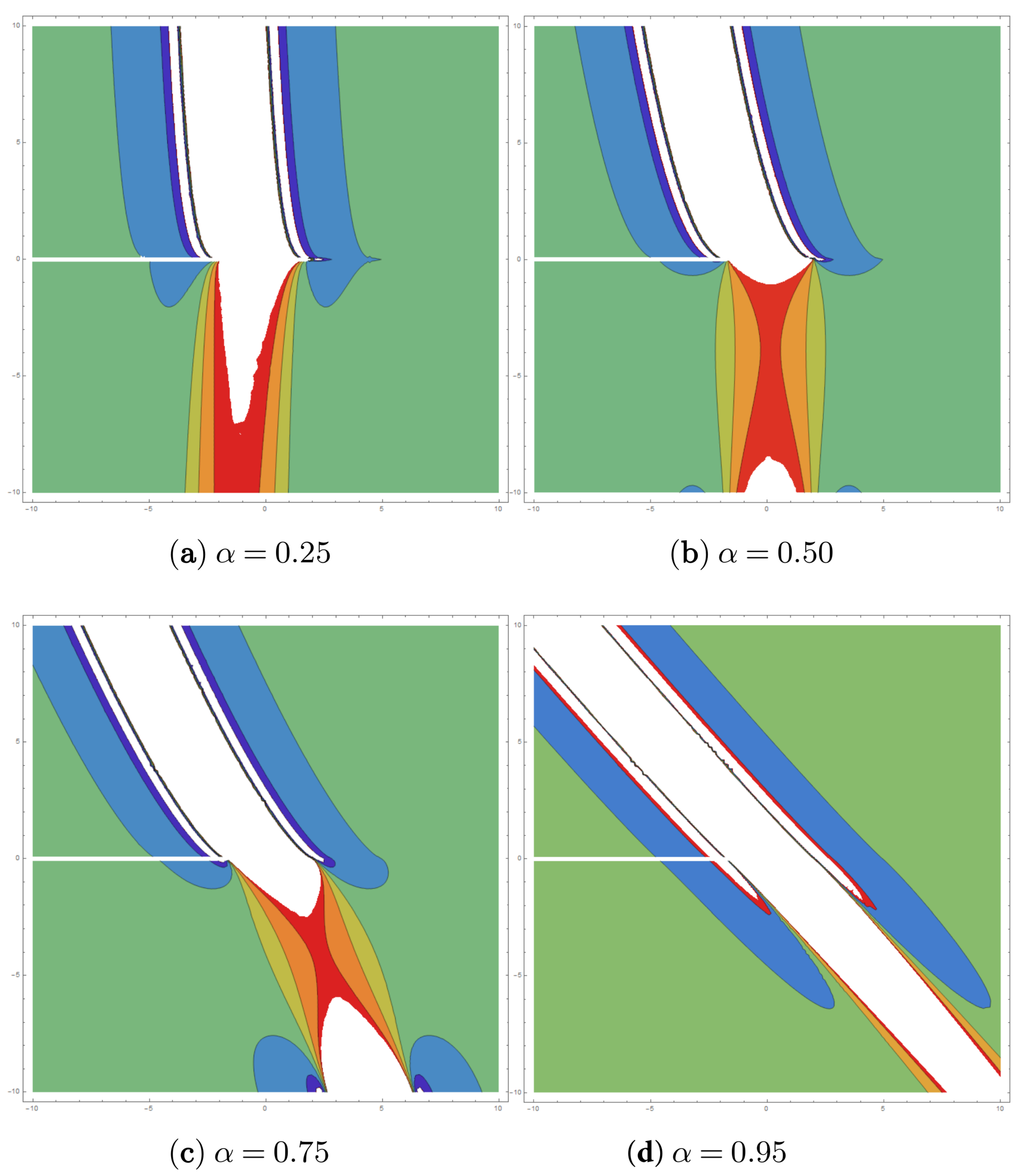
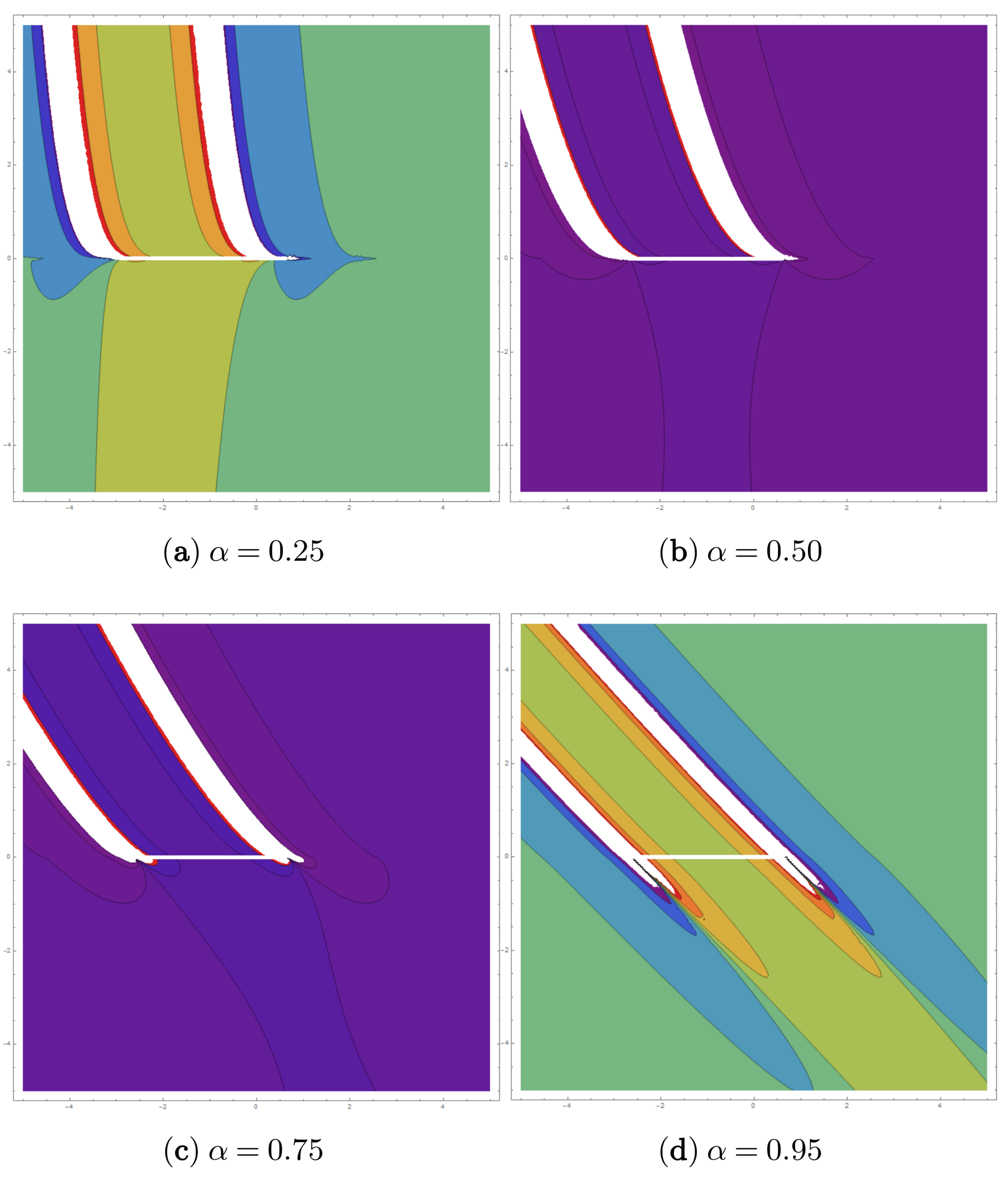
Figure 4.
The 2D-contour graphs for .
Figure 4.
The 2D-contour graphs for .
A direct explanation of is depicted in one such graphic. Here is a graphical depiction of the test assuming the parameters, , , , , , , , while (red), (yellow), (blue), and (green), within the interval
Figure 5.
A 2D graphical representation for .
Figure 5.
A 2D graphical representation for .
Figure 6.
A 3D graphical representation for .
Figure 6.
A 3D graphical representation for .
Figure 7.
The 2D-contour graphs for .
Figure 7.
The 2D-contour graphs for .
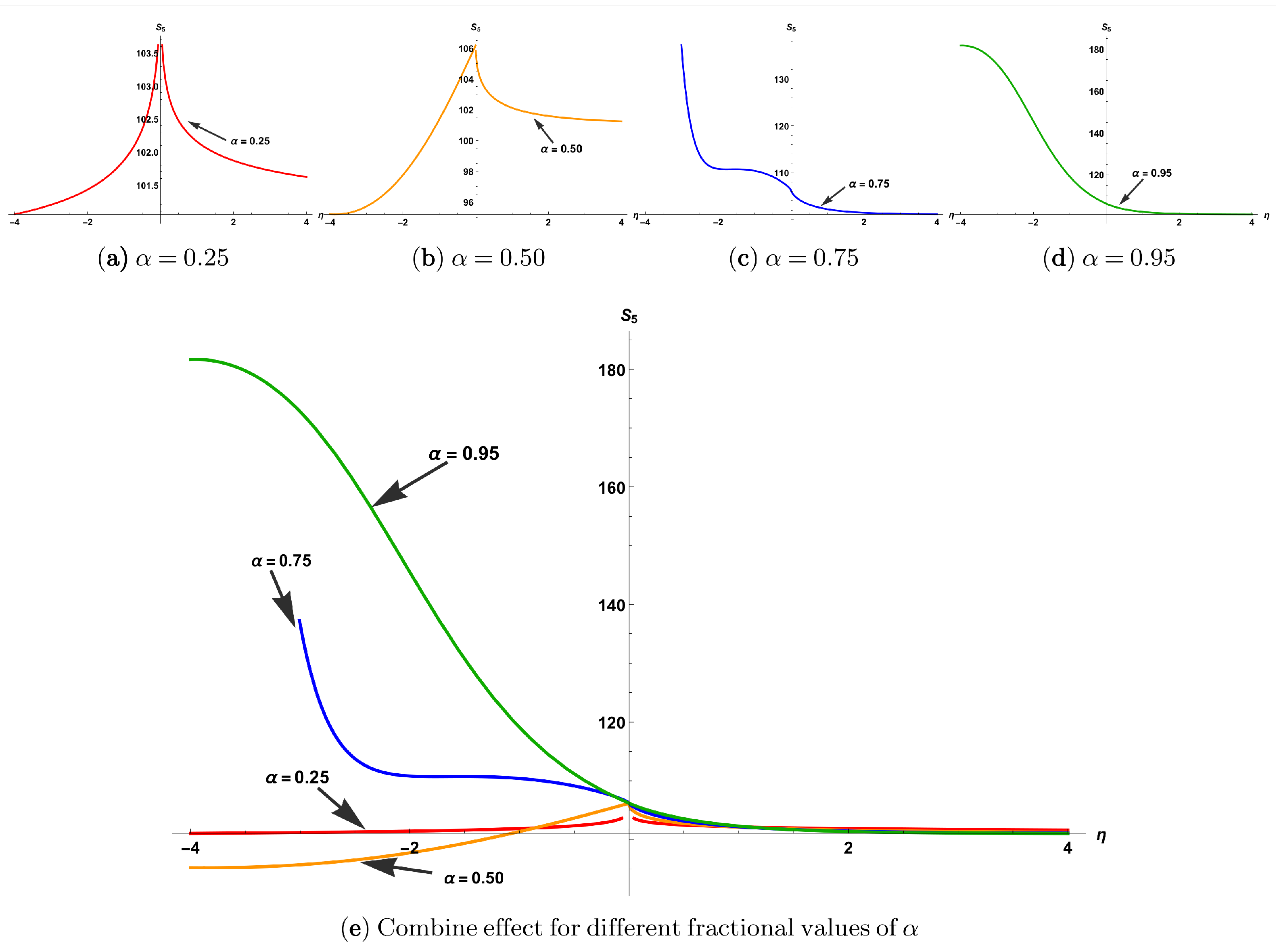
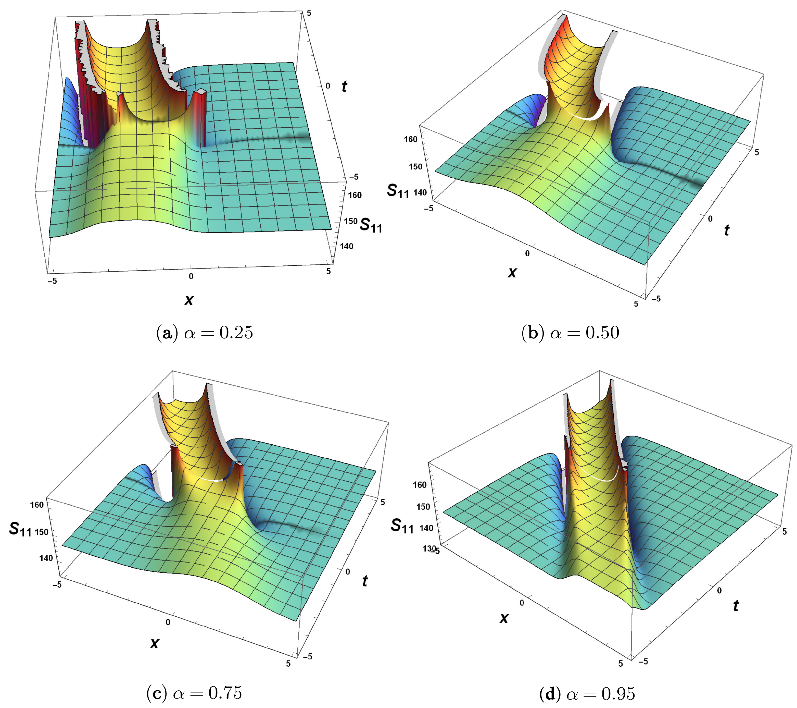
A direct explanation of is depicted in one such graphic. Here is a graphical depiction of the test assuming the parameters, , , , , , , , while (red), (yellow), (blue), (green), with in the interval
Figure 8.
A 2D graphical representation for .
Figure 8.
A 2D graphical representation for .
Figure 9.
A 3D graphical representation for .
Figure 9.
A 3D graphical representation for .
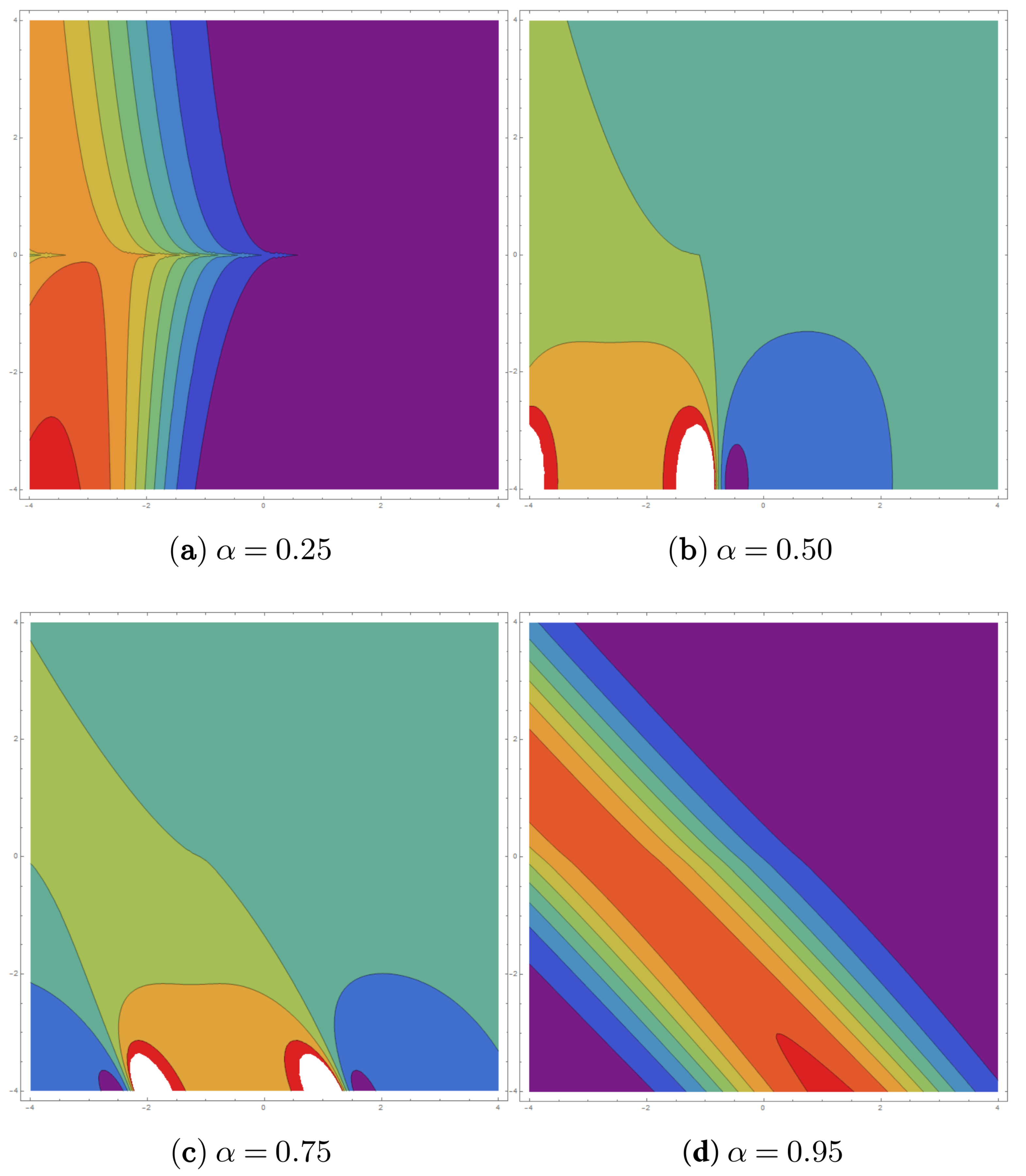
Figure 10.
The 2D contour graphs for .
Figure 10.
The 2D contour graphs for .
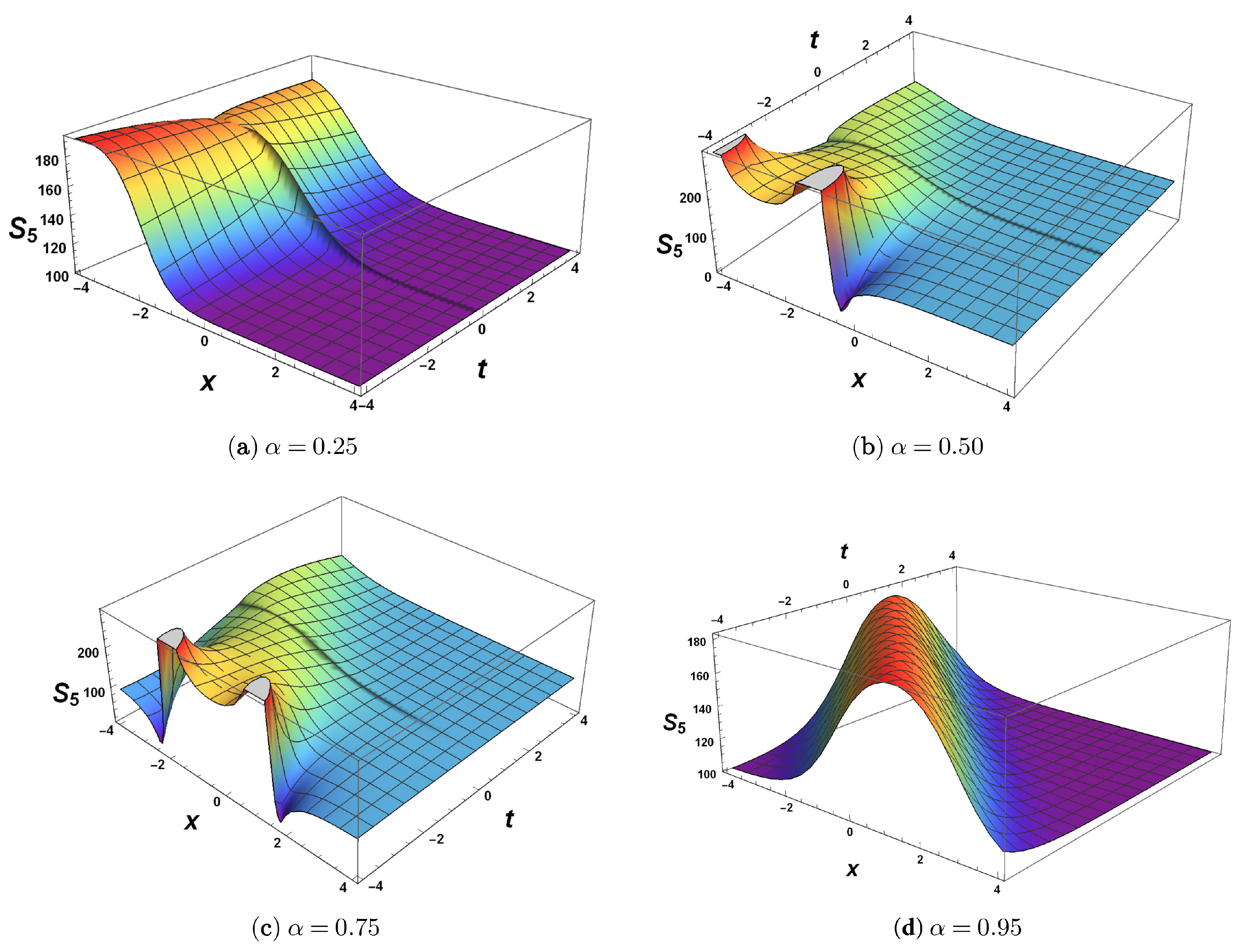
A direct explanation of is depicted in one such graphic. Here is a graphical depiction of the test assuming the parameters, , , , , , , , while (red), (yellow), (blue), and (green), within the interval
Figure 11.
A 2D graphical representation for .
Figure 11.
A 2D graphical representation for .
Figure 12.
A 3D graphical representation for .
Figure 12.
A 3D graphical representation for .
Figure 13.
The 2D-contour graphs for .
Figure 13.
The 2D-contour graphs for .
Proposition: By using the generalized auxiliary equation technique, new varieties of exact traveling wave solutions have been uncovered, comprising the hyperbolic trigonometric, trigonometric, exponential, and rational. We obtain the bright, dark, periodic, singular, and other soliton solutions to this nonlinear model. Some of the achieved solutions are illustrated graphically to understand their physical behavior fully. These are the new results obtained, illustrated in the figures for physical understanding.
6. The Sensitivity Assessment
From Equation (
31), we have the system given below:
From Equation (
46), we can write the following:
where,
,
,
,
.
By using the Galilean transformation, the Equation (
3) can be written by a planar dynamical system as follows:
We examine the sensitive behavior of the perturbed system in
Table 1 given below. Following that, the schemes of Equation (
47) are decomposed in an autonomous conservative dynamical system
, illustrated below:
In the above,
f shows the frequency, and
is the strength of the perturbed component [
31]. There exists a perturbation term in the system Equation (
49) rather than the system given by Equation (
48). We can analyze whether the frequency term impacts the model under study. To this analysis, we assume different values of these terms and analyze their physical properties. Finally, we want to investigate the sensitivity behavior for the perturbed dynamical structural scheme Equation (
49) by utilizing four different initial conditions for the system:
These involving parameters are not the same for each figure, and these are the same for both figures mentioned below. The parametric values are given below:
For
Figure 14a,b,
,
,
,
,
,
,
,
,
,
,
,
,
,
.
For
Figure 14c,d,
,
,
,
,
,
,
,
,
,
,
,
,
,
.
Sensitivity is the determination of the sensitiveness of our system. If a small change in the initial conditions results in a small change in a system, then the system is lowly sensitive. Therefore, if the system undergoes a significant modification as a result of modest change within the initial conditions, the system is very sensitive. The following figures show alternation in the amplitude pattern of waves, indicating that these curves are not overlapped, indicating that the system is sensitive therein.
In
Figure 14a, the plot shows the sensitivity illustrating the dynamical system (
49) assuming the similar parameters as stated earlier for the initial constraints as
in red dotted curve and
throughout the solid blue line. The system has very low sensitivity from the beginning (i.e., 0 to 2) and the system has no sensitivity (i.e., 2 to 20). Alternately, it has some sensitivity in a small region and no sensitivity in a large region.
Figure 14b is a plot of the sensitivity showing the dynamical system (
49) taking the same parameters as stated earlier for the initial constraints as
in the red dotted curve and
in the solid blue line. The system has very low sensitivity from the beginning (i.e., 0 to 2), and the system has no sensitivity for the large range and then is sensitive alternatively.
Figure 14c shows the sensitivity for the mentioned initial conditions as
in the red dotted curve and
throughout the solid blue line. The system has high sensitivity from beginning to end (i.e., 1 to 50). Here, the parameter values are changed and are mentioned above.
Figure 14d is the plot for the sensitivity with initial conditions as
in the red dotted curve and
throughout the solid blue line. The system has high sensitivity from beginning to end (i.e., 1 to 50). Here, the parameters values are changed and are mentioned above.
It is important to note that we have the choice of the initial conditions on hit and trial bases. So, there is no proper method to obtain the sensitivity analysis of the obtained dynamical system. The sensitivity analysis calculations take a lot of data points and time the evaluation. We have taken some of the data points and specified the domain for the sensitive behavior.
Quasi Periodic Behaviors
We will examine the quasi-periodic behavior of the perturbed system given below. Following that, the schemes of Equation (
47) are decomposed in the autonomous conservative dynamical system
, as illustrated below:
In the above,
f shows the frequency, and
is the strength of the perturbed component [
31]. It is the characteristic of a dynamical system which shows the irregular periodicity of the wave. In this part, we discuss the qausi-periodic patterns for the non-autonomous oscillatory system.
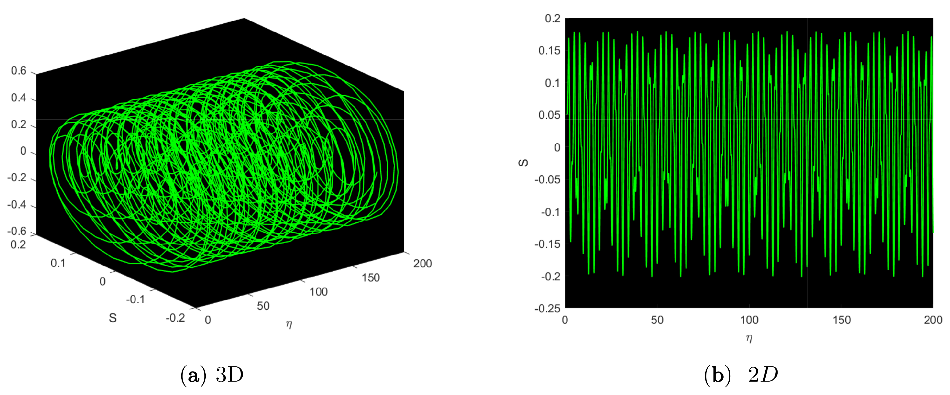
Figure 14 reveals the 3D and 2D phase portraits for the perturbed system Equation (
50) for certain values of
,
,
,
, and
and with the initial condition
and
. From this figure, it is clear that it has a quasi-periodic behavior.
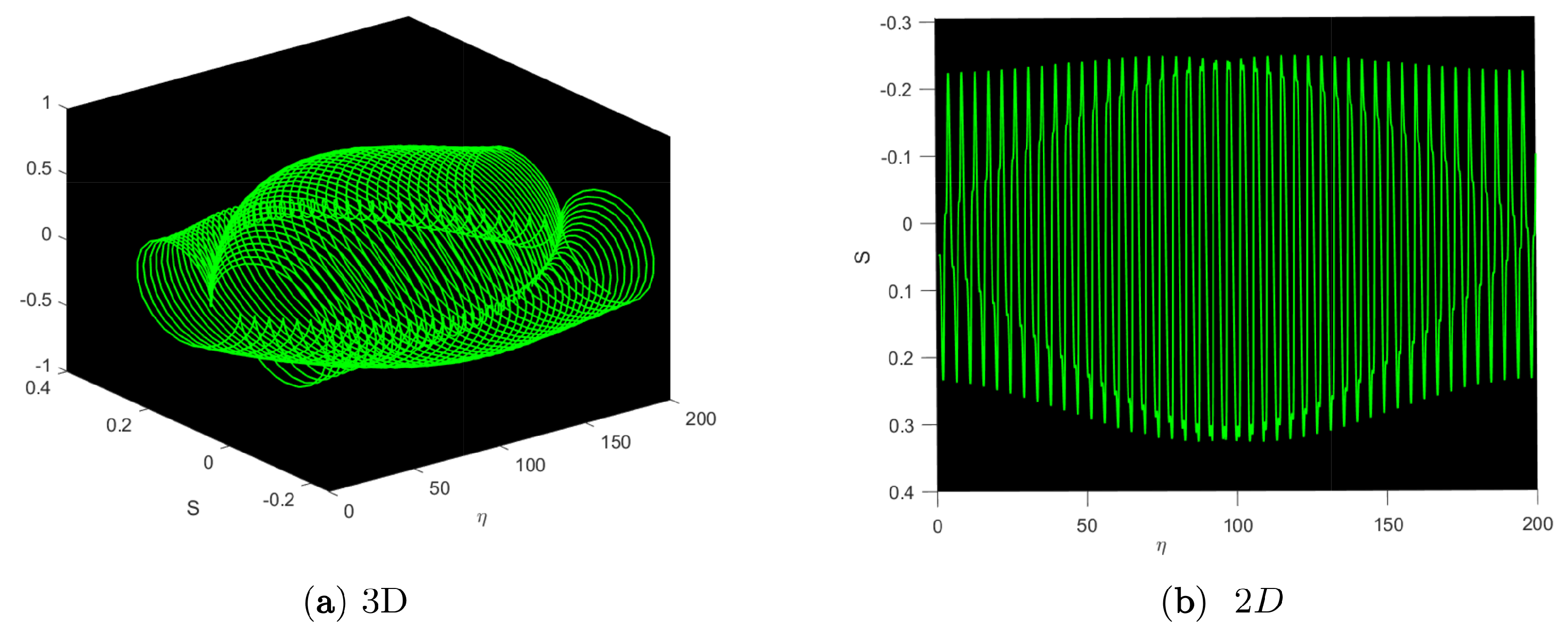
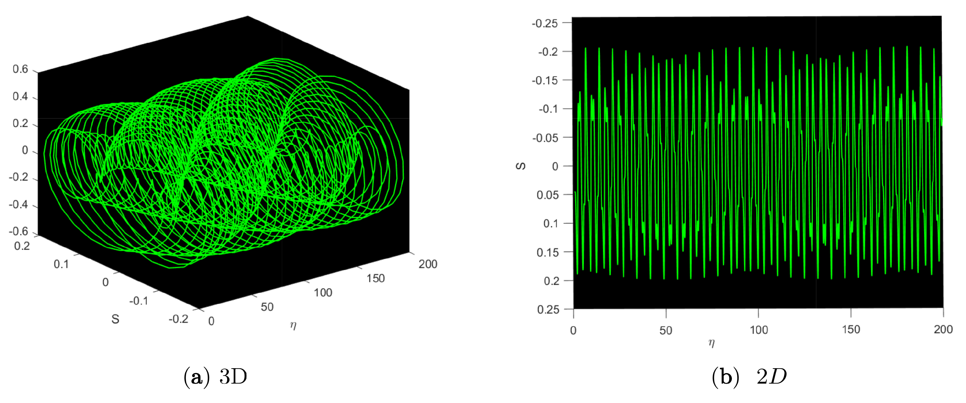
Figure 15,
Figure 16 and
Figure 17 show the 3D and 2D phase portrait for the perturbed system Equation (
50) for different values of
,
,
,
and
f with the same initial condition as
Figure 14.
7. Conclusions
This study seeks to determine soliton solutions for an inherent fractional discrete NETL in a lattice. Our goal here was predicated on the concept that a FO time derivative would be added throughout the Ohm law of such capacitor electrical characteristics for such a realistic network. Therefore, we created a non-integer order (NPDE) for such voltage dynamics using Kirchhoff’s rules for the model under study. It was discovered that such FO time derivatives and the coupling values impacted the performance of newly generated soliton solutions. We demonstrated that, regardless of form, the fractional order changes the transmission velocity of a voltage wave, thus setting up a localized framework across low coupling coefficient quantities. Consequently, at a large amount of such a coupling factor, the non-integer order is less visible in the forms of the newly discovered solitary structures. GAEM drove us to these solitary solutions while employing the mRL derivatives and the fractional complex transform.
A comparable number of papers employing the fractional derivative parameter was published, with particularly good findings. Through adjusting the magnetic coupling coefficients (MCC) in ref. [
32], the authors were able to generate a dark solitons interaction. The influence of the fractional derivative parameter and the MCC on the purchased soliton solutions as well as the modulation instability (MI) enhancement in the Heisenberg ferromagnetic spin was demonstrated in ref. [
33], using the auxiliary equation approach. Numerous mathematical models were used in these publications and transformed into the identical sort of ODE, which resulted in different answers after transformation. Because the methodology is the same, the function we obtain is mathematical functions that are the same, but we obtain different graphs, owing to the various parameter choices.
The sensitivity examination seems to be a process that estimates how sensitive our system is. If the system experiences a modest modification, simply a response to slight changes in the beginning circumstances, the system’s sensitivity is minimal. Hence, the complete study suggests that the chosen approach is a powerful productivity tool for assuring a wide variety of traveling wave solutions to an intrinsic fractional discrete nonlinear electrical transmission lattice occurring in science, engineering, and mathematical physics. In carrying out future studies, these solutions are also very inspiring. We clearly outlined graphically the physical presentation of the results obtained. As GAEM, one of the most powerful frameworks is to discuss the different categories of precise optical lone solutions. A reasonably short and straightforward review informs us that the solutions presented are unique and truly distinctive. The study results presented in the paper are fresh yet not documented in the publications.


