Article

Applications of Prabhakar-like Fractional Derivative for the Solution of Viscous Type Fluid with Newtonian Heating Effect

1
Department of Mathematics, University of Engineering and Technology, Lahore 54890, Pakistan
2
Department of Mathematical Sciences, Faculty of Science and Technology, Universiti Kebangsaan Malaysia, UKM Bangi, Bangi 43600, Malaysia
3
Department of Mathematics and Social Sciences, Sukkur IBA University, Sukkur 65200, Pakistan
4
Department of Mathematical Sciences, Federal Urdu University of Arts, Science & Technology, Gulshan-e-Iqbal, Karachi 75300, Pakistan
5
Department of Mathematics and Statistics, College of Science, Taif University, P.O. Box 11099, Taif 21944, Saudi Arabia
6
Department of Mathematics, Faculty of Science, Khon Kaen University, Khon Kaen 40002, Thailand
7
Laboratory of Nano-Smart Materials for Science and Technology (LNSMST), Department of Physics, Faculty of Science, King Khalid University, P.O. Box 9004, Abha 61413, Saudi Arabia
8
Research Center for Advanced Materials Science (RCAMS), King Khalid University, P.O. Box 9004, Abha 61413, Saudi Arabia
9
Nanoscience Laboratory for Environmental and Biomedical Applications (NLEBA), Metallurgical Laboratory 1, Department of Physics, Faculty of Education, Ain Shams University, Roxy, Cairo 11757, Egypt
10
Mechanical Engineering Department, College of Engineering, Prince Sattam Bin Abdulaziz University, Wadiad Dawaser 11991, Saudi Arabia
11
Production Engineering and Mechanical Design Department, Faculty of Engineering, Mansoura University, Mansoura 35516, Egypt
*
Author to whom correspondence should be addressed.
Fractal Fract. 2022, 6(5), 265; https://doi.org/10.3390/fractalfract6050265
Submission received: 28 March 2022 / Revised: 25 April 2022 / Accepted: 10 May 2022 / Published: 12 May 2022

Abstract

:
This article examines a natural convection viscous unsteady fluid flowing on an oscillating infinite inclined plate. The Newtonian heating effect, slip effect on the boundary wall, and constant mass diffusion conditions are also considered. In order to account for extended memory effects, the semi-analytical solution of transformed governed partial differential equations is attained with the help of a recent and more efficient fractional definition known as Prabhakar, like a thermal fractional derivative with Mittag-Leffler function. Fourier and Fick’s laws are also considered in the thermal profile and concentration field solution. The essentials’ preliminaries, fractional model, and execution approach are expansively addressed. The physical impacts of different parameters on all governed equations are plotted and compared graphically. Additionally, the heat transfer rate, mass diffusion rate, and skin friction are examined with different numerical techniques. Consequently, it is noted that the variation in fractional parameters results in decaying behavior for both thermal and momentum profiles while increasing with the passage of time. Furthermore, in comparing both numerical schemes and existing literature, the overlapping of both curves validates the attained solution of all governed equations.

1. Introduction

Natural convection viscous fluid flows flowing on a vertical plate are widely considered in the literature because of their massive solicitations in different fields of engineering and ecological processes. They are also concentrated in manufacturing submissions such as nuclear reactors, filtration methods, spaceship design, fiber insulation, geothermic schemes, etc. Numerous investigators have examined unsteady natural convective flows past an oscillating and vertical plate with different thermal imposed conditions. Georgantopoulos [1] was the first who find a closed-form solution for natural convection impacts on the flow of a viscous fluid along with a vertical plate. The naturalconvection flows of a viscoelastic fluid with an accelerated plate were discussed by Raptis and Singh [2]. The impacts of the magnetic field were also reserved for contemplation. Free convection impacts considering an exponentially accelerated and infinite vertical plate were deliberated in [3]. Natural convection wavering flow past an infinite permeable plate and continuous suction were considered through Soundalgekar [4]. The communication of natural convection and the vibrating flow with vertical plate and thermal radiation can be seen in [5]. The impacts of heat contamination on the boundary layer with a horizontal plate were examined by Ishak [6,7]. Haq et al. [8] calculated the closed-form solutions of MHD natural convection flow past along a vertical and oscillating plate with thermal flux in a permeable medium with integral transforms.In [9], the authors studied the flow between two parallel plates with the non-isothermal slip effect of a non-linear model. Different parameters with slip coefficients in thermal profiles have also been considered. A non-uniformly heated viscous fluid flow model flowing through a bounded domain was studied by Baranovskii et al. [10].
Natural convection flows have fascinated extensive consideration because of their importance in many fields of science containing biomedical engineering and fluid dynamics. It is often momentous in refrigeration, atmospheric as well as oceanic circulation, concentration, spaceship structure, dehydration, filtration, ventilation of building plan, processing of permeable materials in textile workshops, conserving systems and electronic things for nuclear-powered plants, nuclear reactors, cooled or heated storing places, electric power strategies, and solar collectors [11]. The natural convection mechanism happens because of significant temperature alterations, which can impact the density of the fluid and then source relative buoyancy of the fluid. It has abundant applications in numerous scientific as well as industrial concerns. Natural convection in various systems, actions, and tools is incredibly momentous in exothermal reactions tasks. It is suitable for security attention under different circumstances, where the typical mode continues to flop and when the procedure trusts natural convection to dispose of the designed temperature. It has unusual significance in energy production and digital devices and systems in which such an arrangement is compulsory to avoid extreme heat [12]. In the last few years, extensive analytical and theoretical studies on natural convection have been conducted to understand several environmental features and phenomena in considered frequent scientific circumstances. Javaid et al. [13] deliberated the free convection flowed based on second-grade fluid and stated that with the Grashof number and Prandtl number, the velocity for viscous fluid was more than the velocity estimations of second-grade fluid. The electro-osmotic flow analysis for second-grade fluids and slip conditions was effectively discoursed through Wang et al. [14]. Closed-form solutions were found utilizing integral transform. Numerous particular cases prevailing in the literature were also improved. The natural convection flow of fractional incompressible and second-grade fluid along two upright plates was discussed in the radiation effect between both plates, and an analytical solution was attained by Nisa et al. [15]. The prior studies may perceive countless research topics on the natural convection flow models [16,17,18,19,20,21,22].
In the last few years, fractional calculus has been promising because of its massive implication in different fields of engineering and applied sciences that are not present in the fields of non-fractional calculus, which agrees with a random order of differentiation as well as integration. Ali et al. [23,24], Nehad et al. [25], and Zafar et al. [26] exploited different new definitions of fractional derivatives for the solutions of different Newtonian and non-Newtonian type fluids. Imran et al. [27] utilized the AB-fractional model to excavate out the semi-analytical solution of the Maxwell fractional model. Nadeem et al. [28] examined the AB and CF factional model and attained an analytical solution of Casson-type nanofluid. Various physical phenomena constructed on differential equations with fractional calculus are immensely used for the modeling of numerous everyday life physical problems, as fractional calculus takes memory impacts, such as problems in relaxation, oscillation, diffusion, fluid flow, retardation, dynamical processes, engineering processes, where classical models cannot predict the previous state of processes [29,30,31,32,33,34].
The construction of numerous physical phenomena consequences increases the complexity of partial differential equations. The calculation of solutions for such complicated equations is significant in investigating such physical phenomena. Fractional calculus is the critical division of mathematics that effectively reports diverse methods for the simulation of such types of problems. The complex mathematical expressions, including the local and non-local kernels, can be efficiently tackled through a fractional approach. The Caputo–Fabrizio (CF) and Atangana–Baleanu (AB) methods are the most well-known apparatuses in fractional calculus that different investigators have extensively applied in past years. Tialk Raj Prabhakar was an Indian mathematician who proposed a novel three-parameter fractional operator:the Mittag-Leffer function with three different fractional operators. This Mittag-Leffer operator successfully applies conventional kernels [35]. Sulaiman et al. [36] found the solution for Burger’s equation through diverse fractional derivatives comprising MLF kernels. AB and CF fractional derivatives and Mittag-Leffer and exponential functions were compared [37]. Singh et al. [38] studied the Cattaneo–Christov derivatives and solved fractional diffusion equations by exploiting the Hilfer–Prabhakar operator. Samraiz et al. [39] deliberated the (k,s)-Hilfer–Prabhakr fractional operator for diverse types of mathematical fractional problems. In [40], Basit et al. employed the Prabhakar fractional technique to examine the solution of second-grade fractional nanofluid, taking different types of nanoparticles. Rehman et al. [41] studied the free convection Maxwell fluid flow under the Newtonian heating effect using the Prabhakar fractional derivative technique of the Mittag-Leffler function, in which they also considered Fourier and Fick’s law to investigate the solution of thermal and concentration profiles. In [42], the authors inspected the free convection fluid flow with generalized thermal transport and carbon nanotubes as nanoparticles using a recent fractional derivative definition.
The main focus of current research is to study the natural convection, incompressible, viscous, and unsteady flow on an infinite oscillating inclined plate under the influence of an applied inclined magnetic field in the sense of the Prabhakar fractional derivative operator. Newtonian heating influences are engaged into focus in the fractional thermal flow model to check the thermal performance. The Prabhakar fractional derivative operator technique with Laplace transform is followed to accomplish the fractional and numerical simulations. To achieve the inverse of the Laplace method, two important diverse methods T’zous method and Stehfest, are applied. In the end, the thermal results are enumerated for different flow characters.

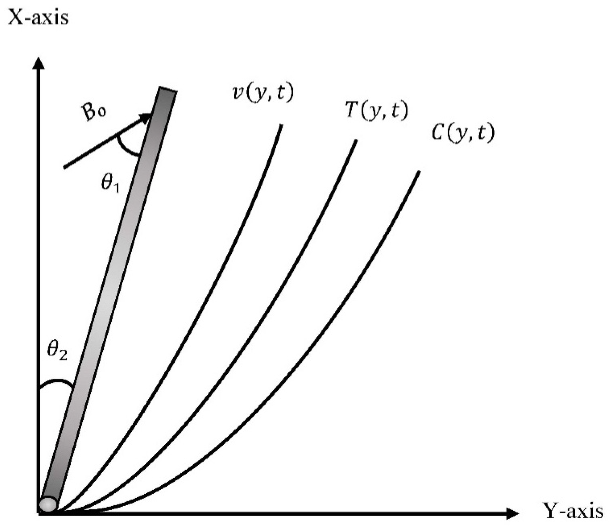
2. Problem Description

Suppose a natural convection, incompressible, viscous, and unsteady flow on an infinite oscillating inclined plate under the impact of the applied inclined magnetic field with strength B o . As the inclined plate is in the xy-plane, therefore, all the governed equations are functions of y and t. Initially, at t = 0 , the inclined plate and fluid are both in a constant situation with a constant temperature T and concentration of C . With time   t > 0 + , the fixed plate starts to oscillate with particular continual velocity f ( t ) , with f ( 0 ) = 0 , and temperature and concentration levels also rise with time, as shown in Figure 1. In light of the above conditions and neglecting the viscous dissipation and pressure gradient, the governed partial differential equations with their physical boundary conditions can be modeled by Boussinesp’s approximation as follows [43].
v ( y , t ) t = ν 2 v ( y , t ) y 2 σ B o 2 ρ s i n ( θ 1 ) v ( y , t ) + g β T ( T ( y , t ) T ) C o s ( θ 2 ) + g β C ( C ( y , t ) C ) C o s ( θ 2 )
ρ C p T ( y , t ) t = δ ( y , t ) y
δ ( y , t ) = k T ( y , t ) y
C ( y , t ) t = J ( y , t ) y K ( C ( y , t ) C )
J ( y , t ) = D C ( y , t ) y
With its dependable physical boundary conditions, as follows
v ( y , 0 ) = 0 ,   T ( y , 0 ) = T ,   C ( y , 0 ) = C ;   y 0
v ( 0 , t ) h v ( y , t ) y | y = 0 = U o f ( t ) ,   T y | y = 0 = h k T ( 0 , t ) ,   C ( 0 , t ) = C w ;   t > 0
v ( y , t ) 0 ,   T ( y , t ) T ,   C ( y , t ) C   a s   y
where δ ( y , t ) , J ( y , t ) identifies the thermal flux rate by Fourier’s law and Fick’s law, respectively. Now, the non-dimensional governing Equations (1)–(5) and the corresponding consistent conditions present the subsequent non-dimensional values:
v * = k ν h v ,   y * = h k y ,   t * = g k ν h t ,   T * = T ( y , t ) T T w T ,   R e = ν 2 g ( h k ) 3
C * = C ( y , t ) C C w C ,   K * = K ν g ( h k ) ,   q * = q q o ,   J * = J J o
into the proceeding governed equations and forgetting the “*” notation. We attain the succeeding non-dimensional formulas as
v ( y , t ) t = R e 2 v ( y , t ) y 2 M s i n ( θ 1 ) v ( y , t ) + G r C o s ( θ 2 ) T ( y , t ) + G m C o s ( θ 2 ) C ( y , t )
P r e f f T ( y , t ) t = δ ( y , t ) y
δ ( y , t ) = T ( y , t ) y
S c e f f C ( y , t ) t = J ( y , t ) y K S c e f f C ( y , t )
J ( y , t ) = T ( y , t ) y
with the following dimensionless physical conditions
v ( y , 0 ) = 0 ,   T ( y , 0 ) = 0 , C ( y , 0 ) = 0 ;   y 0
v ( 0 , t ) h v ( y , t ) y | y = 0 = f ( t ) ,   T ( y , t ) y | y = 0 = ( 1 + T ( 0 , t ) ) ,   C ( 0 , t ) = 1
v ( , t ) 0 ,   T ( , t ) 0 ,   C ( , t ) 0 ;   t > 0  
where
P r = μ C p κ ,   G r = g ( υ β T ) f ( T w T ) ν o 2 ,   S c = ν D , P r e f f = P r R e , S c e f f = S c R e
The Navier slip coefficient and Newtonian heating effect are also considered in the above-mentioned physical conditions of the flowing fluid and the fluid temperature, concentration, and velocity will be zero at y . This article will discuss a generalized mathematical model in which the memory effect and shear stress are also under consideration in the sense of the Prabhakar fractional operator. The respective mathematical preliminaries will define the basic concept of the fractional scheme and the relation of the Prabhakar fractional technique with other fractional models.
Basic preliminaries:
The one-parametric MittagLeffler function with mathematical form as
E α ( z ) = n = 0 z n Γ ( α n + 1 ) ;   α , z ,   R e ( α ) > 0
was studied by Mittag-Leffler [44]. Then after some time, Wiman [45] explored the more generalization form of the one-parametric function, known as two-parametric Mittag-Leffler functions with the mathematical form as follows:
E α , β ( z ) = n = 0 z n Γ ( α n + β ) ;   α , z , β ,   R e ( α ) > 0
In [46], authors introduced the three-parametric Mittag-Leffler function, which is commonly known as the Prabhakar fractional derivative
E α , β γ ( z ) = n = 0 ( γ ) n z n n !   Γ ( α n + β ) ;   α , β , γ , z ,   R e ( α ) > 0
with the basic properties
E α ( z ) = E α , 1 1 ( z ) ,   E α , β ( z ) = E α , β γ ( z ) ,   E 1 , 1 1 ( z ) = exp ( z )
{ t β 1 E α , β γ ( α t α ) } = q β ( 1 α q α ) γ
(Prabhakar kernel) The function
e α , β γ ( α ; t ) = t β 1 E α , β γ ( α t α ) ;   t ,   α , β , γ , z
is identified as the Prabhakar kernel.
(Prabhakar Integral) The Prabhakar integral can be defined as [47,48]
E α , β , α γ f ( t ) = e α , β γ ( α ; t ) f ( t ) = 0 t ( t τ ) β 1 E α , β γ ( α ( t τ ) α ) f ( τ ) d τ
with its Laplace transform
{ E α , β , α γ f ( t ) } ( q ) = { e α , β γ ( α ; t ) } { f ( t ) } = q α γ β ( q α α ) γ { f ( t ) }
Some applicable fractional constraint cases can be encapsulated as
If β = γ = 0
1 { { e α , 0 0 ( α ; t ) } } = 1 { 1 } = δ ( t )
If β = 1 ,   γ = 0
1 { { e α , 1 0 ( α ; t ) } } = 1 { 1 q } = 1
If β > 0 ,   γ = 0
1 { { e α , β 0 ( α ; t ) } } = 1 { 1 q β } = t β 1 Γ ( β )
when β > 0 ,   α = 0 , then the property three repeats as
{ e α , β γ ( 0 ) } = q β
(The regularized Prabhakar derivative) In [47,48], the regularized Prabhakar derivative is distinct as
D C α , β , α γ g ( t ) = E α , m β , α γ g m ( t ) = 0 t ( t τ ) m β 1 E α , m β γ ( α ( t τ ) α ) g m ( τ ) d ( τ )
E α , β γ ( z ) = n = 0 Γ ( γ + n ) z n n ! Γ ( γ ) Γ ( α n + β )
where D C α , β , α γ signifies the Prabhakar derivative operator and g m represents the mth derivative of g ( t ) . The Laplace transformation of generalized Prabhakar and its kernel can be derived as
{ D C α , β , α γ g ( t ) } = { e α , m β γ ( α ; t ) g m ( t ) } { g m ( t ) } = q β m ( 1 α q α ) γ { g m ( t ) }
{ e α , m β γ ( α ; t ) } = q β m ( 1 α q α ) γ
The primary relations and connections with different fractional operators can be encapsulated as follows.
  • When β 0 ,   γ = 0 , the Prabhakar derivative will transform into the Caputo derivative D C α , β , α 0 g ( t ) = D C t β g ( t ) .
  • When α = β = 1 ,   γ = 1 , then the relation between Prabhakar and CF derivative will become D C 1 , 1 , σ 1 σ g ( t ) = g ( t ) σ D C F t σ g ( t ) .
  • When β = 1 ,   γ = 1 ,   0 < α < 1 , then the connection between the AB derivative and Prabhakar derivative will develop as D C α , 1 , σ 1 σ 1 g ( t ) = ( 1 α ) d d t D A B C t α g ( t ) .
  • When β = γ = 0 ,   m = 0 , the Prabhakar derivative will be D C α , 0 , α 0 g ( t ) = g ( t ) with its kernel h ¯ p ( α , 0 , 0 , α , q ) = 1 .
  • When β = 1 ,   γ = 0 ,   m = 1 , the Prabhakar derivative D C α , 1 , α 0 g ( t ) = g ( t ) with its kernel h ¯ p ( α , 1 , 0 , α , q ) = d d t ( g ( t ) ) . As the LT of Prabhakar, fractional operator D C α , β , α γ is, consequently,
[ D C α , β , α γ   h ( t ) ] = [ h m ( t ) e α , m β γ ( α ; t ) ] = { h m ( t ) } { e α , m β γ ( α ; t ) } = { h m ( t ) } s β m ( 1 α s α ) γ
We may obtain the traditional Fourier’s law by taking   β = γ = 0 . Moreover, because Fourier’s law of thermal conductivity primarily determines the Prabhakar fractional derivative, Fourier and Fick’s laws in the context of the Prabhakar derivative are as follows.
δ ( y , t ) = D C α , β , α γ T ( y , t ) y
J ( y , t ) = D C α , β , α γ C ( y , t ) y

3. Solution of the Problem

3.1. Solution of the Energy Profile

Appling the LT on transformed Equations (10) and (21) and utilizing its matching conditions for the solution of the energy profile
P r e f f q T ¯ ( y , q ) = q β ( 1 α q α ) γ 2 T ¯ ( y , q ) y 2
T ¯ ( y , q ) y | y = 0 = ( 1 q + T ¯ ( 0 , q ) ) ,   T ¯ ( y , q ) 0 ;   y
By inserting these transmuted conditions, the solution of the thermal profile is as follows:
T ¯ ( y , q ) = q β ( 1 α q α ) γ P r e f f q q β ( 1 α q α ) γ e y P r e f f q q β ( 1 α q α ) γ q
We employ numerical approaches, namely, Stehfest and Tzou’s schemes in Table 1 and Table 2, to analyze the inversion of Equation (25).

Classical Solution of the Energy Field ( β = γ = 0 )

For the classical solution of thermal profile take β = γ = 0 , so
[ e α , 0 0 ( α ; t ) ] = 1 = δ ( t )
δ ( t ) denotes the Dirac’s Delta distribution. Due to this, the generalized Fourier’s law is changed into classical Fourier’s law. Additionally,
T ¯ ( y , q ) = 1 P r e f f q 1 e y P r e f f q q
with its Laplace inverse
T ( y , t ) = h 1 ( t ) h 2 ( t )
h 1 ( t ) = 1 { 1 P r e f f q 1 } = 1 P r e f f ( 1 π t + e t P r e f f E r f c [ t P r e f f ] P r e f f )
h 2 ( t ) = 1 { e y P r e f f q q } = E r f c [ P r e f f y 2 t ]

3.2. Solution of the Concentration Profile

With the same methodology as used for the energy field, utilizing the LT on Equations (12) and (22),
2 C ¯ ( y , q ) y 2 S c e f f ( K + q ) q β ( 1 α q α ) γ C ¯ ( y , q ) = 0
C ¯ ( y , q ) = 1 q ,   T ¯ ( y , q ) 0 ;   y
Using the above conditions and after simplification, the solution of Equation (28) becomes
C ¯ ( y , q ) = 1 q e y S c e f f ( K + q ) q β ( 1 α q α ) γ
Again, the inversion of Laplace of the above equation is examined numerically in Table 1 and Table 2.

Classical Solution of the Concentration Profile ( β = γ = 0 )

For the classical solution of the concentration profile, again, take β = γ = 0 .
The generalized Fick’s law is changed into classical Fick’s law as a result of this.
C ( y , t ) = 1 2 e K S c e f f y ( 1 + Erf [ 2 K t S c e f f y 2 t ] + e 2 K S c e f f y Erfc [ 2 K t + S c e f f y 2 t ] )

3.3. Solution of Momentum Field

In this part, the velocity equation solution is determined using the same approach as the energy equation solution. Using the LT technique on Equation (9) and its accompanying conditions, we obtain
R e 2 v ¯ ( y , q ) y 2 q v ¯ ( y , q ) M s i n ( θ 1 ) v ¯ ( y , q ) = G r C o s ( θ 2 ) T ¯ ( y , q ) G m C o s ( θ 2 ) C ¯ ( y , q )
v ¯ ( 0 , q ) h v ¯ ( y , q ) y | y = 0 = F ( q ) ,   v ¯ ( y , q ) 0 ;   y
Employing these conditions, the solution of the momentum equation turns out to be
v ¯ ( y , q ) = 1 1 + h 1 R e ( q + M s i n ( θ 1 ) ) ( G r c o s ( θ 2 ) R e q q β ( 1 α q α ) γ P r e f f q q β ( 1 α q α ) γ 1 + h P r e f f q q β ( 1 α q α ) γ P r e f f q q β ( 1 α q α ) γ 1 R e ( q + M s i n ( θ 1 ) ) + G m c o s ( θ 2 ) R e q 1 + h S c e f f ( K + q ) q β ( 1 α q α ) γ S c e f f ( K + q ) q β ( 1 α q α ) γ 1 R e ( q + M s i n ( θ 1 ) ) + F ( q ) ) e y 1 R e ( q + M s i n ( θ 1 ) ) G r c o s ( θ 2 ) R e q q β ( 1 α q α ) γ P r e f f q q β ( 1 α q α ) γ e y P r e f f q q β ( 1 α q α ) γ P r e f f q q β ( 1 α q α ) γ 1 R e ( q + M s i n ( θ 1 ) ) G m c o s ( θ 2 ) R e q e y S c e f f ( K + q ) q β ( 1 α q α ) γ S c e f f ( K + q ) q β ( 1 α q α ) γ 1 R e ( q + M s i n ( θ 1 ) )
Nusselt number, Sherwood number, and skin friction are as follows:
N u = T ( y , t ) y | y = 0 = 1 { T ¯ ( 0 , q ) y }
S h = C ( y , t ) y | y = 0 = 1 { C ¯ ( 0 , q ) y }
C f = v ( y , t ) y | y = 0 = 1 { v ¯ ( 0 , q ) y }
Various writers have utilized various numerical inverse methods to calculate the Laplace inverse. Recently, Ali et al. [33], and Tiwanaet al. [49] used the Stehfest and Tzous algorithms for the inversion of Laplace of governed equations solutions. Similarly, Aleem et al. [50], Chu et al. [51], and Asjadet al. [52] also used different numerical techniques for the solution of different hybrid nanofluid, Brinkman type nanofluid, and natural convection flowing fluids. As a result, we additionally employed Stehfestand Tzou’s methods to quantitatively examine the temperature, concentration, and velocity profile solution. Gaver–Stehfest and Tzou’s [53] algorithm can mathematically be inscribed as
w ( ξ , t ) = l n ( 2 ) t n = 1 N v n w ¯ ( ξ , n l n ( 2 ) t )
where N is a positive integer, and
v n = ( 1 ) n + N 2 r = [ q + 1 2 ] m i n ( q , N 2 ) r N 2 ( 2 r ) ! ( N 2 r ) ! r !   ( r 1 ) !   ( q r ) !   ( 2 r q ) !
and
w ( ξ , t ) = e 4.7 t [ 1 2 w ¯ ( r , 4.7 t ) + R e { j = 1 N ( 1 ) k w ¯ ( r , 4.7 + k π i t ) } ]

4. Results and Discussion

This paper investigates the flow of a viscous, incompressible, and unstable fluid under the influence of an angled magnetic field. In order to account for extended memory effects, a fractional model was built using the recently proposed Prabhakar fractional function and a Mittag-Leffler kernel in the governing equations. Then, the solution of all governed equations containing thermal, concentration, and momentum profiles in the sense of Fourier and Fick’s laws is derived using the integral transform scheme, namely Laplace transformation, and various inverse numerical algorithms, i.e., Stehfest and Tzou’s algorithms are used to obtain the Laplace inverse of guided equations. Finally, graphs 2–15 are drawn to investigate the physical impact of different constraints such as α ,   β ,   γ ,   P r e f f ,   S c e f f ,   G r ,   G m ,   R e ,   M and quantitatively investigate the heat transfer rate, mass diffusion rate, and skin friction, which are examined with different numerical techniques in Table 1 and Table 2.
Figure 2 highlights the impact of fractional constraints of the Prabhakar fractional derivatives on the thermal profile for different time values. It can be seen that by increasing the values of fractional parameters, the thermal profile represents the decaying behavior. Using fractional derivatives, it is significant to check the influence of time on governed equations. With time, the fluid temperature increases asymptotically near the plate and has a more significant effect for large values of time. Figure 3 highlights the influence of adequate Prandtl numbers on the thermal field of flowing fluid by fixing other constraints. The figure shows the thermal field representing decaying behavior for adequate Prandtl numbers. Physically, the increment in P r e f f decreases the thermal conductivity of the flowing fluid and increases the viscosity, which decreases the temperature of the flowing fluid. The physical impact of fractional parameters and Schmidt number on the concentration of the boundary layer of the flowing fluid is plotted in Figure 4 and Figure 5 for different time values. Like the thermal profile, again, the variation in fractional parameters and Schmidt number results in a decline in the concentration profile. For large values of the Schmidt number   S c , viscous forces overwhelm the diffusional effects. The Schmidt number represents mass transfer via diffusion and the relative effectiveness of momentum in concentration and speed in free convection flow regimes. As a result, momentum diffusion will effectively counterbalance large values of S c , since molecular diffusivity will be decelerated, and the viscosity effects will be enhanced. As a result, with high S c values, the concentration profile of the boundary layer is reduced.
The effects of fractional parameters on the momentum profile of the flowing fluid are highlighted in Figure 6. It can be seen that the fluid velocity decreases by increasing the value of fractional constraints and increases near the plate with increasing the value oftime and reaches its maximum point; it slowly decreases along the y-axis and reaches zero for higher values of y . The fluid velocity increases near the plate, and the boundary thickness increases with the enhancement in the values of time t. Physically, the increment in the values of factional constraints relates to the thickness of the momentum and thermal profiles. The variation in the values of fractional parameters reduces the thickness of the boundary layer of flowing fluids, due to which the thermal and momentum field shows a decrement trend for this parameter. Figure 7 explains the influence of adequate Prandtl numbers on the momentum profile of the flowing fluid. Again, the momentum field represents decaying behavior with the increment in the value of Prandtl numbers. Physically, the enhancement in the Prandtl numbers means the increment in the viscosity of the fluid and decrement in the thermal conductivity of the flowing fluid, which results in decay in the momentum field of the fluid flow. The variation in velocity profile due to the heat Grashof number and mass Grashof number can be seen in Figure 8 and Figure 9, respectively. Due to the increment in the Grashof number, the buoyancy effect also increases, which increases the thickness of the boundary layer of the fluid, so by varying the values of both parameters, the fluid velocity also increases and shows a unique maximum point near the plate, varying the value of time. In addition, the velocity increases with higher time values and the highest finding near the plate. The fluid motion slows down asymptotically as y increases, satisfying the boundary conditions. Figure 10 and Figure 11 are plotted to see the influence of S c e f f and R e for the velocity profile for different values of the time. An increment in the Schmidt number means a decrease in the molecular diffusion of the boundary layer, which decreases the momentum profile.
The effects of the applied magnetic field and the angle of inclination of the applied magnetic field are examined in Figure 12 and Figure 13. It can be seen that with the variation of both parameters, the momentum profile decays. Physically, the variation in the magnetic field enhances the Lorentz force, resulting in a decrease in the momentum field, and the maximum strength of the applied magnetic field is at the right angle, as shown in the figures. The numerical comparison of concentration, temperature, and momentum profiles with different numerical inversion techniques can be examined in Table 1. They are found to be in good agreement due to the very close results of both numerical techniques. Moreover, the numerical analysis of the heat transfer rate, mass transfer rate, and skin friction at different times is examined in Table 2. It can be predicted that both the Nusselt number (heat transfer rate) and skin friction decrease continuously while increasing with time.

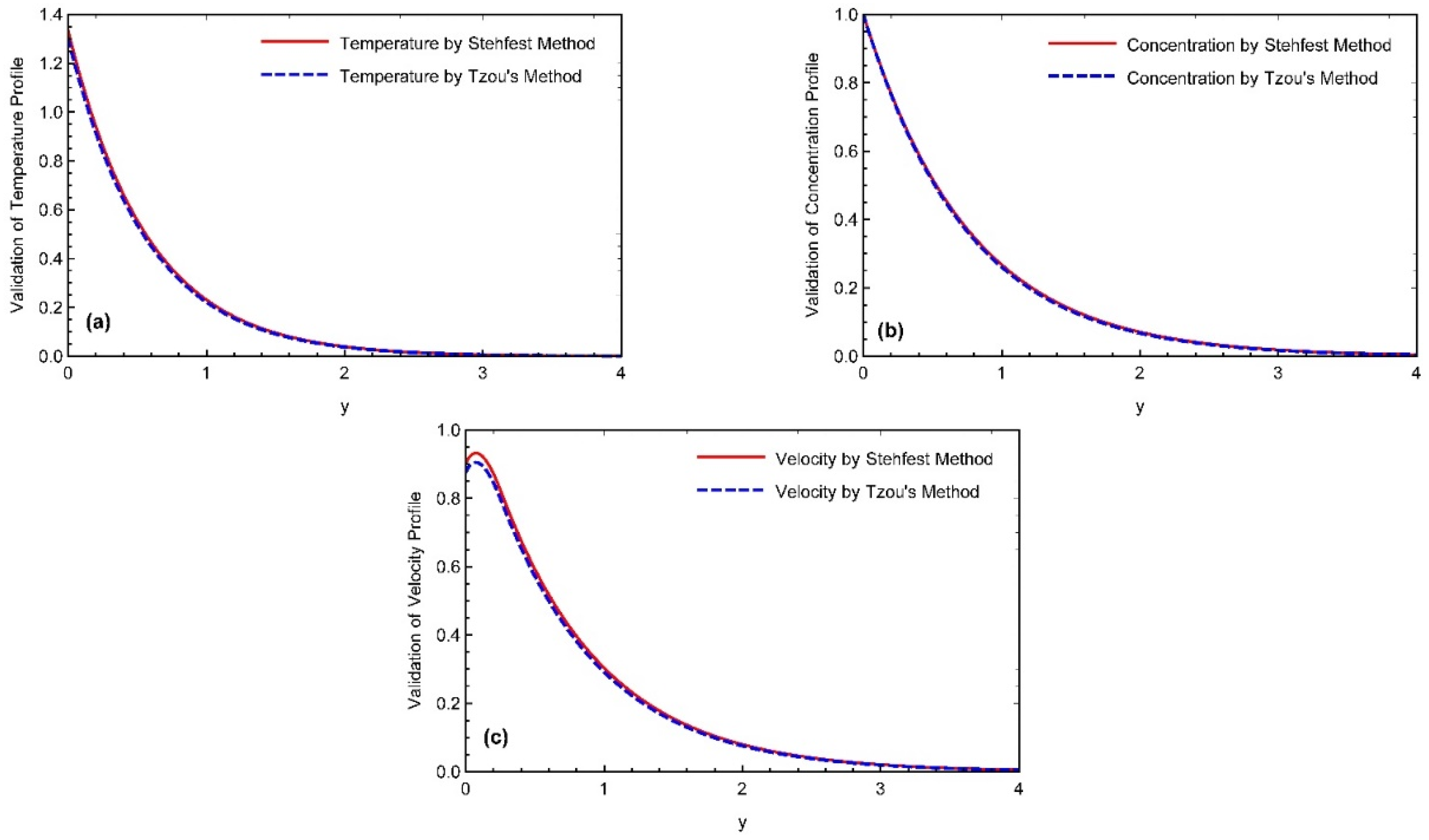
5. Validation of Attained Results

The comparison of the two numerical systems, Stehfest and Tzou’s, is examined by drawing Figure 14a–c for all temperature, concentration, and momentum profiles. A slight overlap of findings between the two curves validates the attained results. In Figure 15a,b, a comparison of the solutions for temperature and velocity fields using the Prabhakar fractional methodology is shown with the work of Imran et al. [54]. The simulations generated by employing the Prabhakar fractional model have good accuracy when compared to the study of Imran et al. [54].

6. Conclusions

The Prabhakar-like thermal fractional technique is used in this study to examine the problem of a viscous, incompressible, and unsteady fluid flowing across an oscillating inclined plate. In order to account for extended memory effects, a recent and more efficient fractional definition, namely the Prabhakar fractional derivative, is utilized with the Mittag-Leffler kernel. Non-dimensional fractional governed equations are solved using the LT approach; an integral transform method, namely the Laplace inverse of governed equations, is computed using a variety of numerical approaches. The impact of various restrictions on leading equations is visually and numerically investigated. The primary outputs derived from graphical and numerical representation can be bulleted as follows:
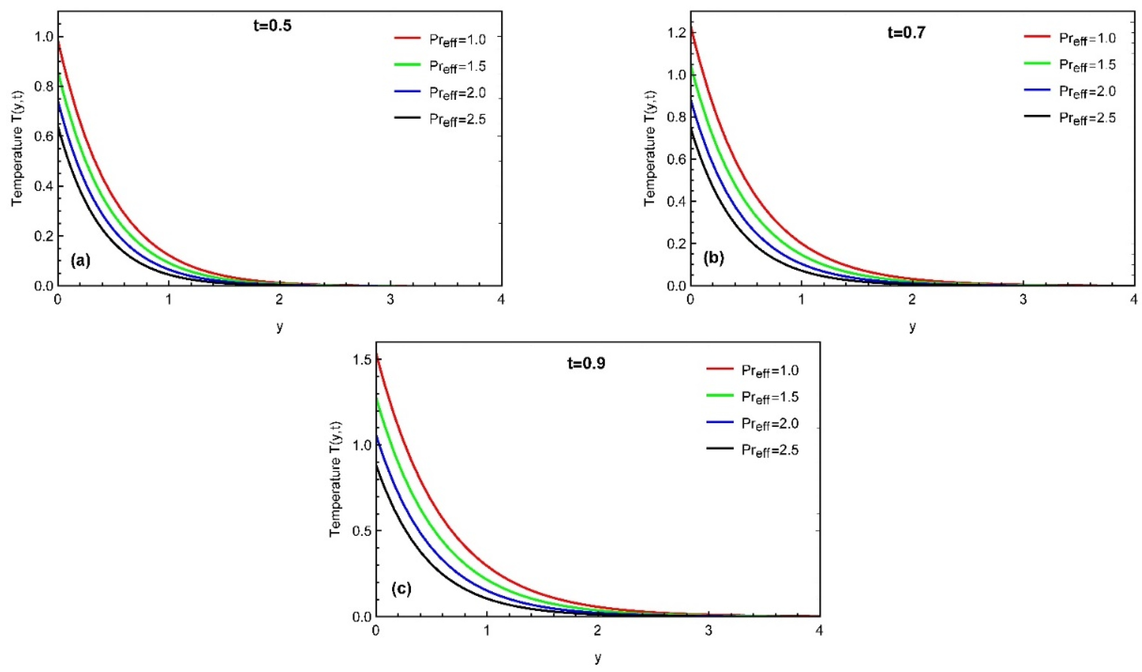
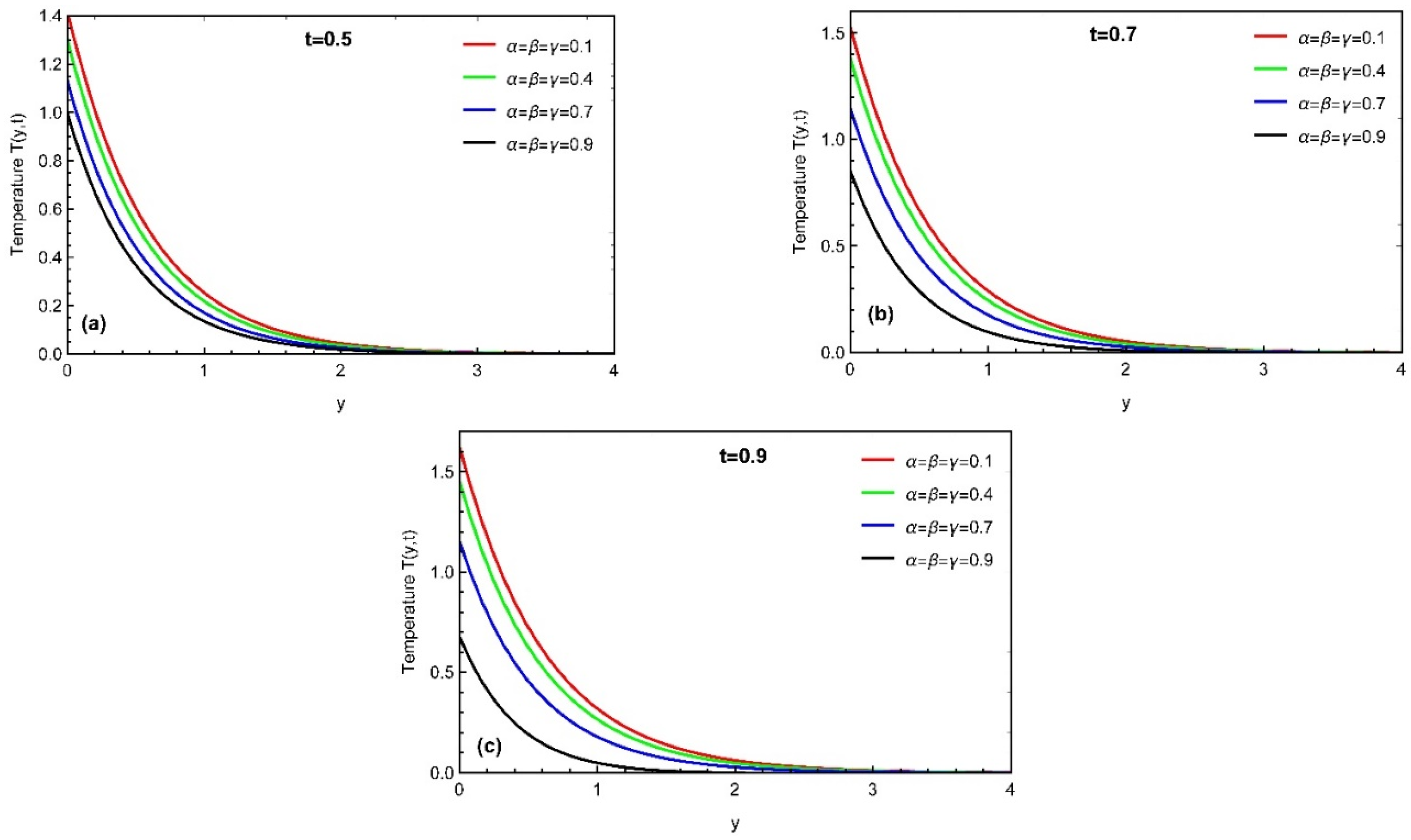
  • The impact of larger values of fractional parameter and an adequate Prandtl number declines the profiles of temperature distributions.
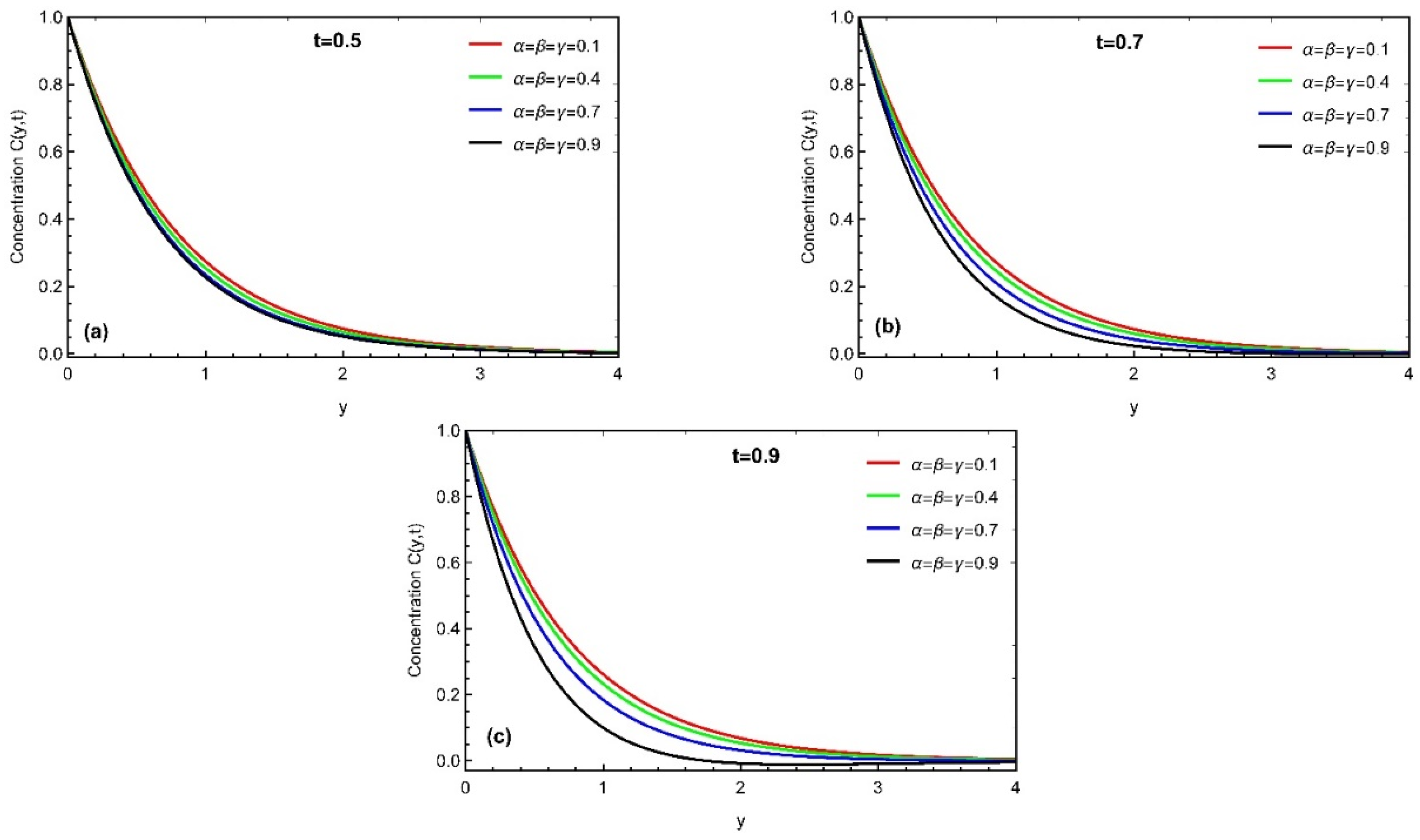
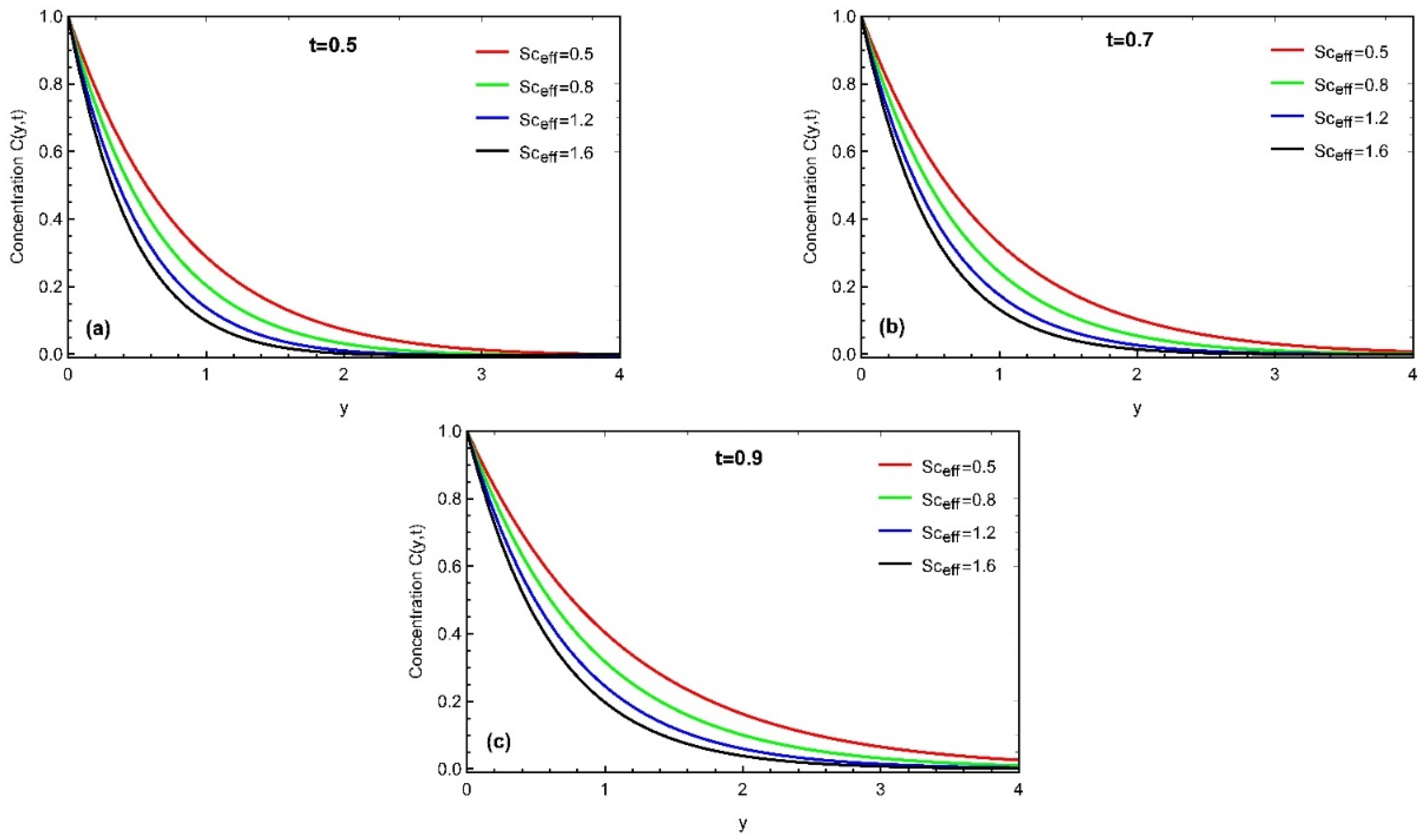
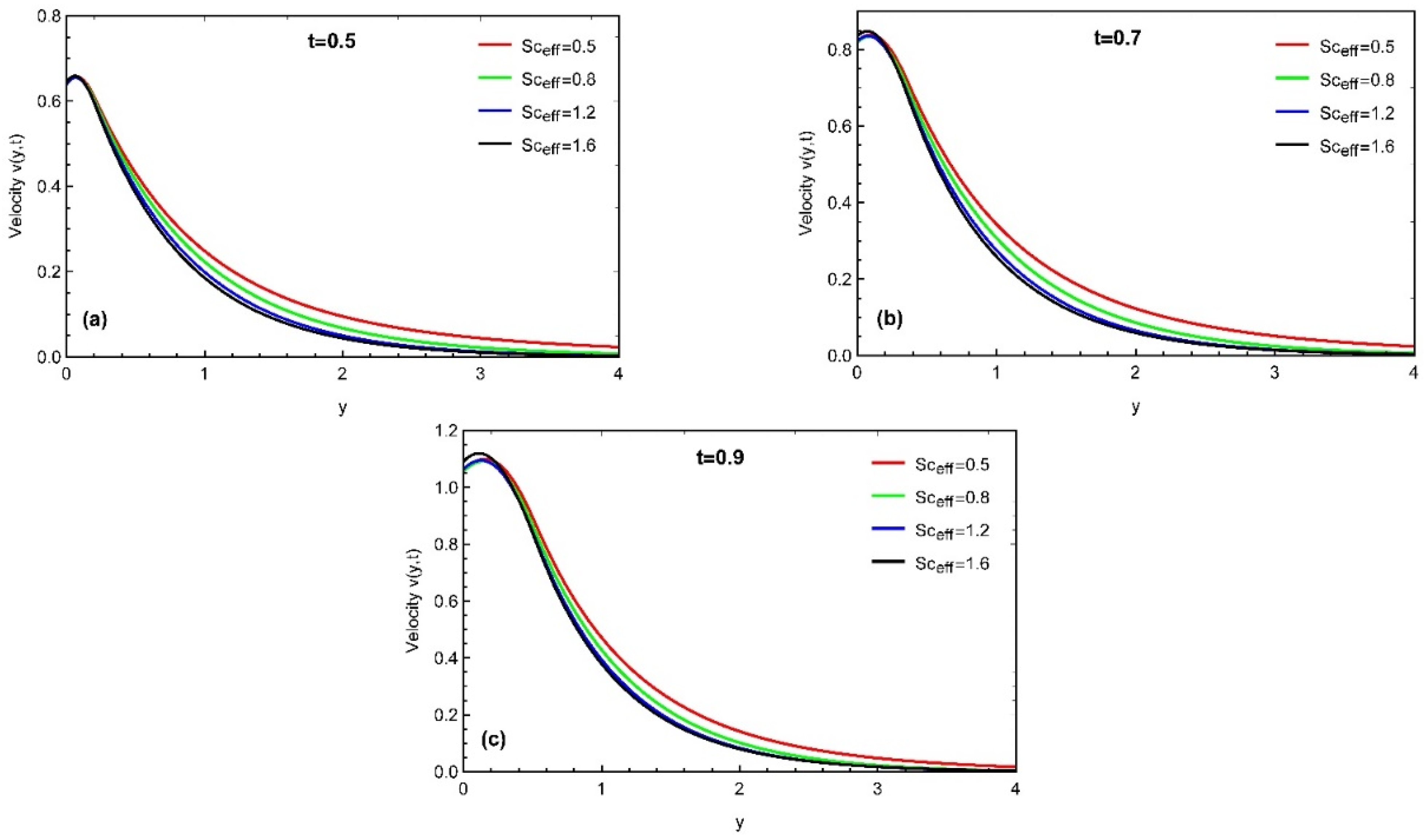
  • The boundary layer concentration also decays with the enhancement in fractional parameter and Schmidt number.
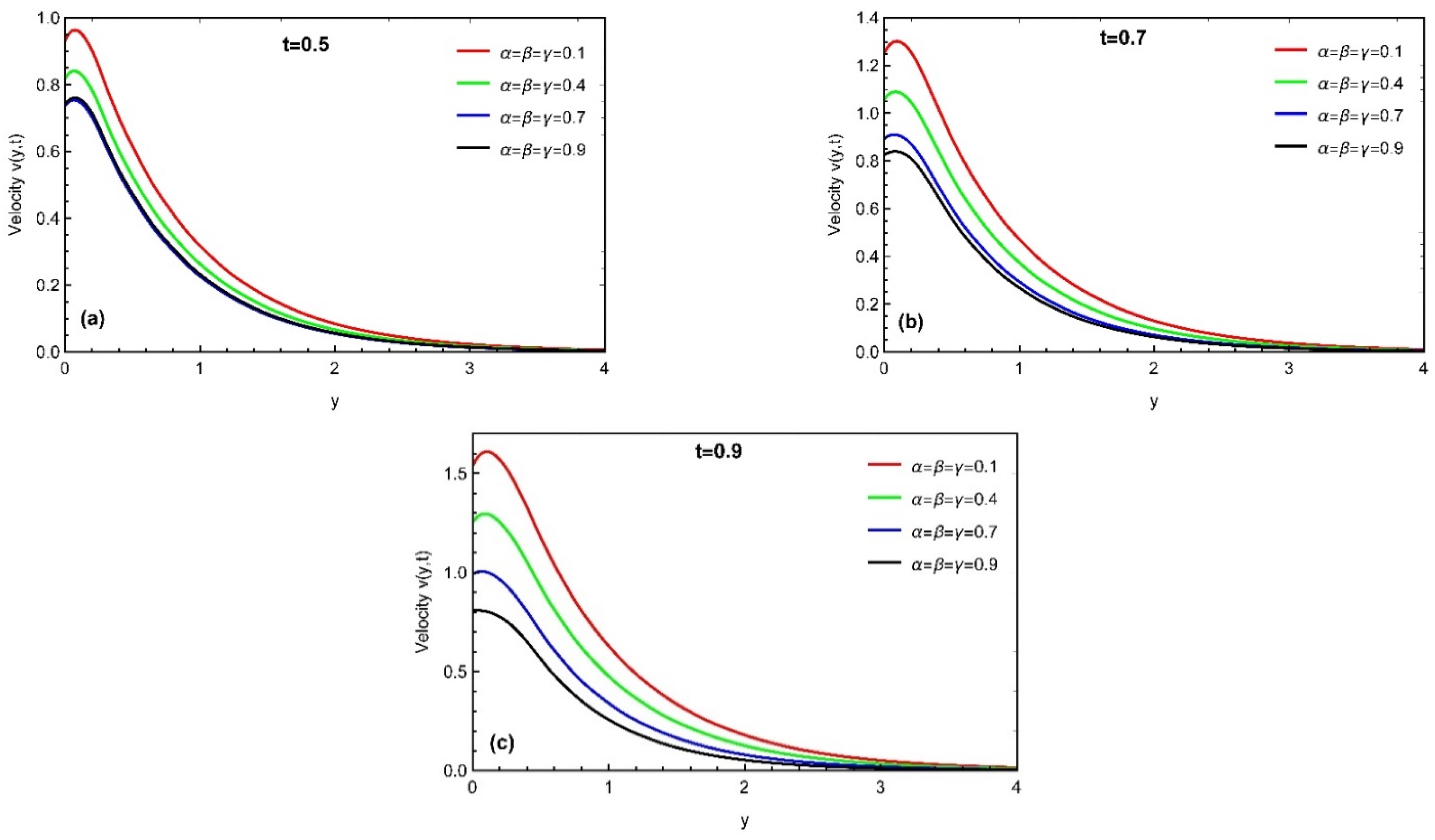
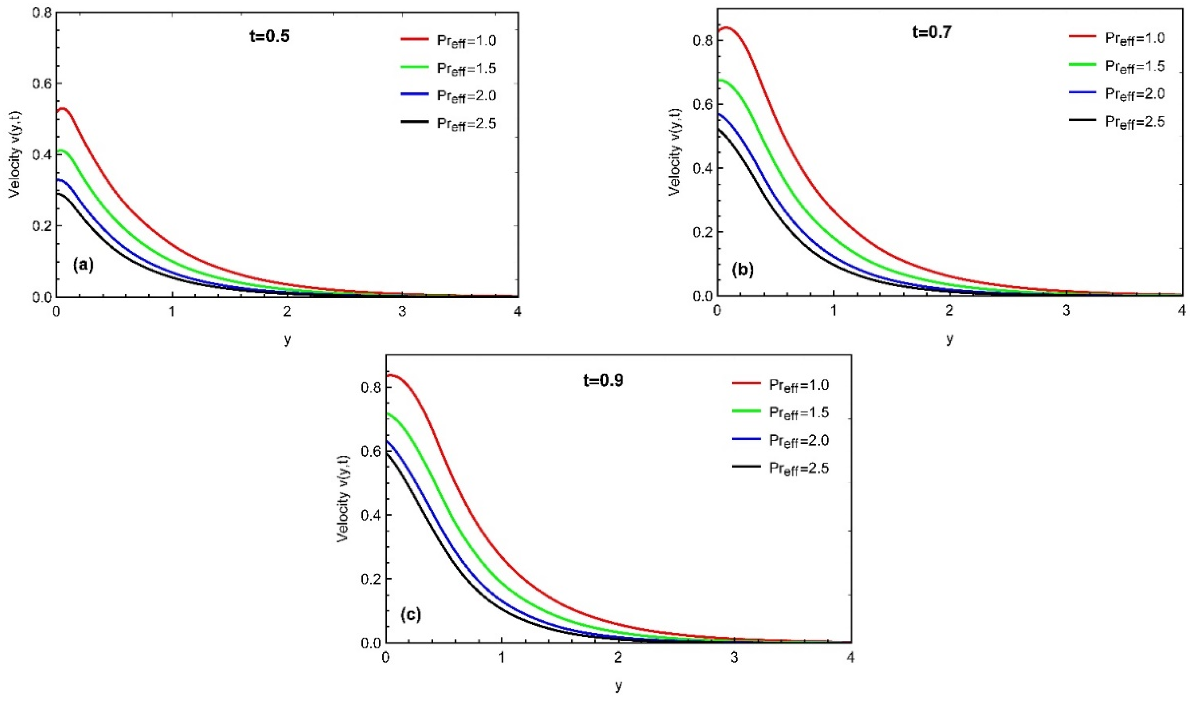
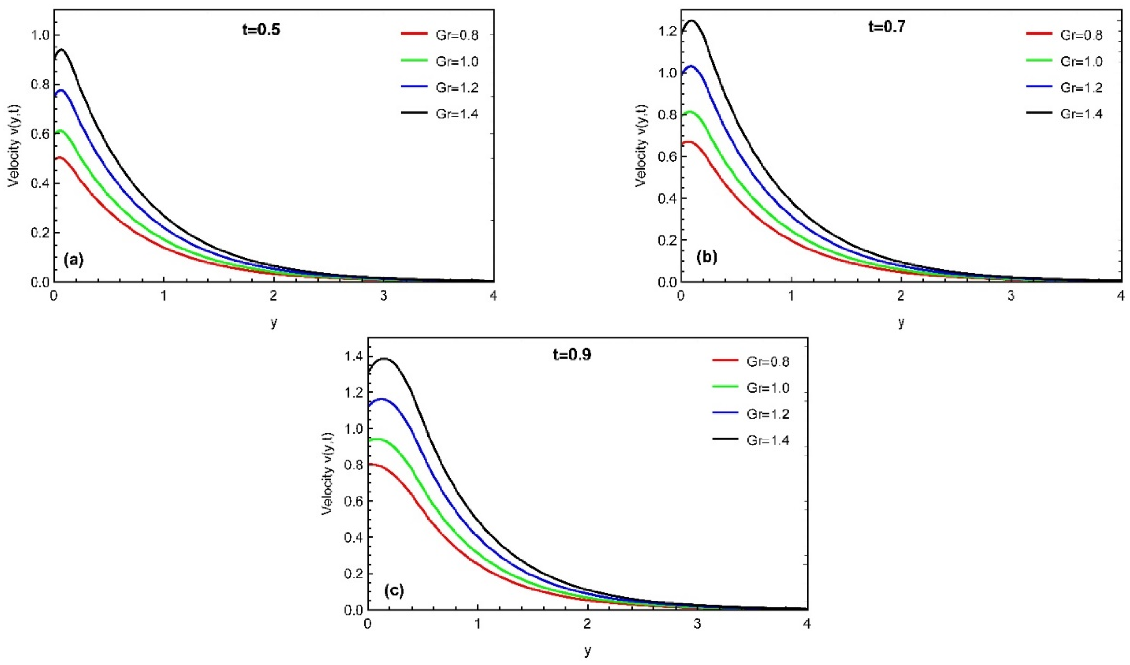
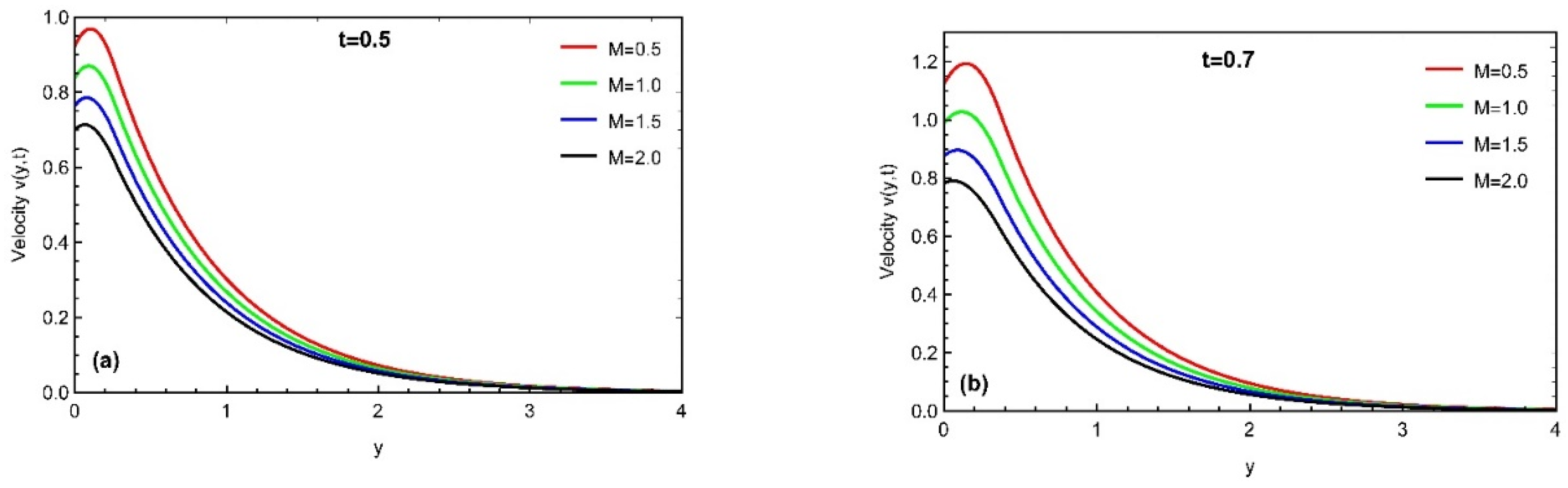
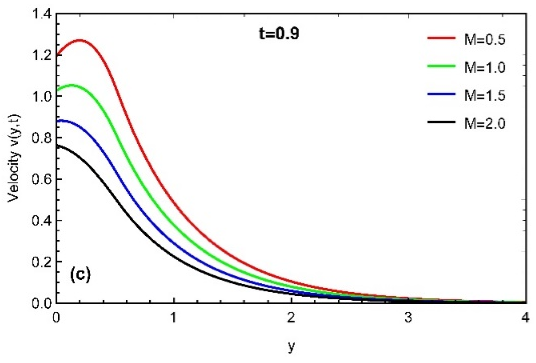
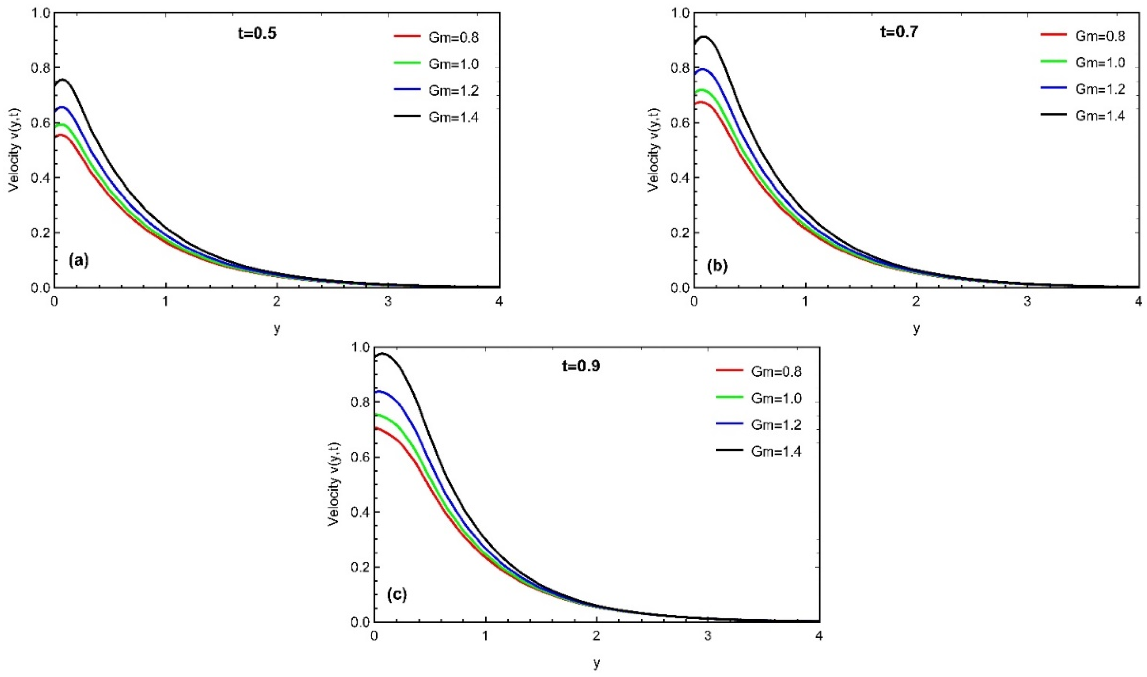
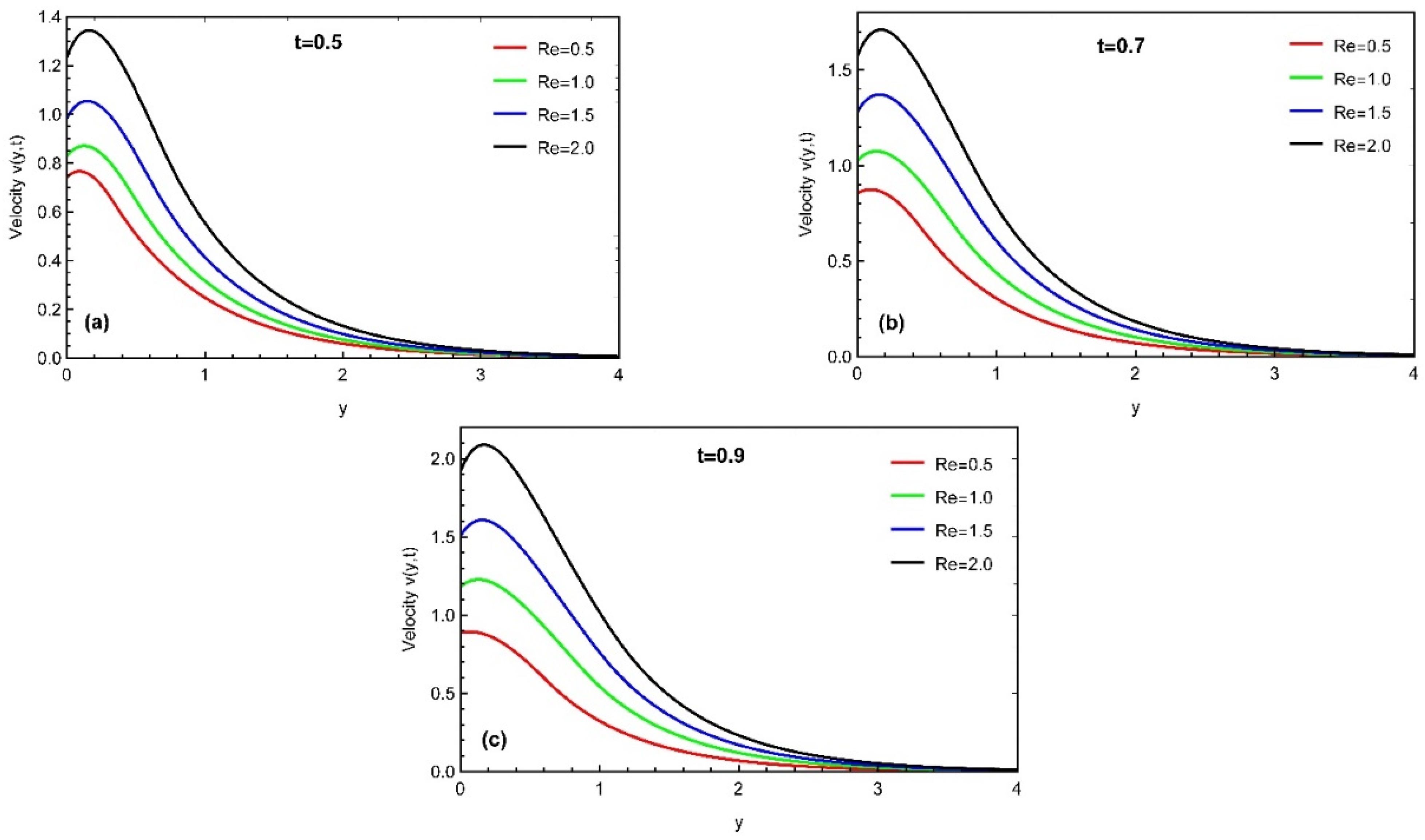
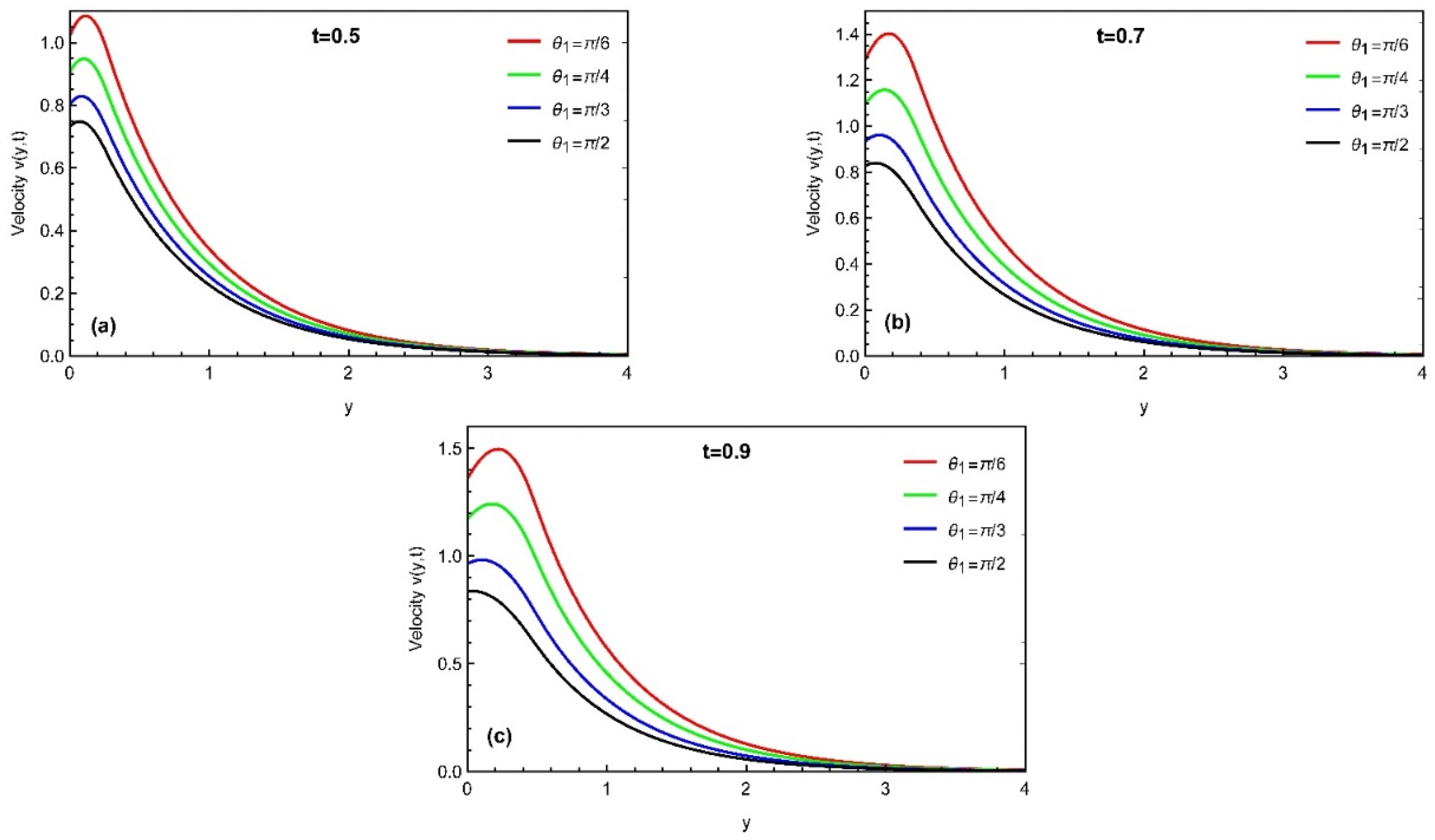
  • The momentum profile is an increasing function for R e ,   G r ,   G m   ,while it decreases with the variation in   P r e f f ,   S c e f f ,   M ,   θ 1 and Prabhakar fractional parameters.
  • Thermal profile, concentration, and momentum profiles asymptotically increase with time.
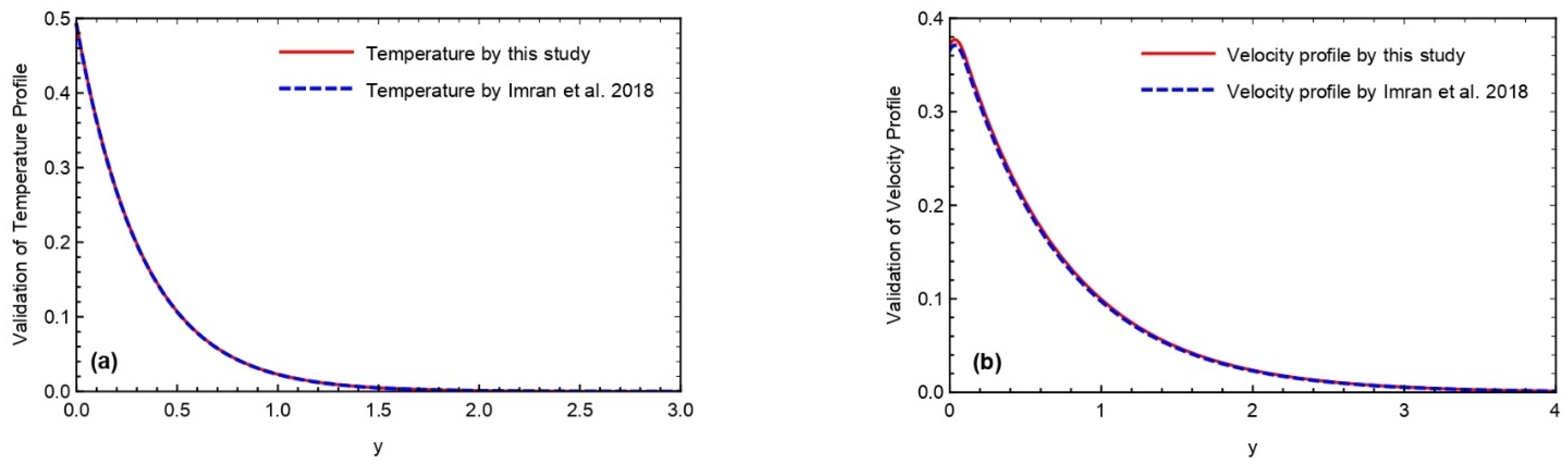
  • The overlapping of both numerical schemes validates the attained solution of all governed equations.
  • The momentum profile is maximal near the plate. It approaches its distinctive peak values in the stream region and then decreases away along the y-axis.
  • The rate of heat transfer, mass transfer, and skin friction varies with the increment in time values.
  • In the comparison of numerical techniques and with the attained results of Imran et al. [54], the overlapping of both curves validates the attained results of this study.
  • As the Prabhakar fractional derivative is the more recent definition of the fractional derivatives technique, it has more efficient and accurate results as compared to other fractional operators as depicted in the comparison of Imran et al. [54].

Author Contributions

Conceptualization, A.R. and U.K.; methodology, A.R. and U.K.; software, A.R., A.Z. and U.K.; validation, A.R., U.K., E.E.M. and W.W.; formal analysis, A.M.G., E.E.M., A.R., I.S.Y., A.Z. and W.W.; investigation, U.K., A.M.G., E.E.M., A.Z. and I.S.Y.; resources, A.M.G.; data curation, A.Z.; writing—original draft preparation, U.K., A.R., E.E.M., I.S.Y. and W.W.; writing—review and editing, A.Z., A.M.G. and I.S.Y.; visualization, A.Z., A.R., I.S.Y., W.W. and U.K.; supervision, A.Z.; project administration, W.W.; funding acquisition, I.S.Y. and E.E.M. All authors have read and agreed to the published version of the manuscript.

Funding

This work received funding from the Deanship of Scientific Research at King Khalid University and the Deputyship for Research & Innovation, Ministry of Education, in Saudi Arabia. Also, this work was supported by Taif University Researchers Supporting Project number (TURSP-2020/20), Taif University, Taif, Saudi Arabia.

Data Availability Statement

Not applicable.

Acknowledgments

The authors express their appreciation to the Deanship of Scientific Research at King Khalid University for funding this work through a research groups program under grant number R.G.P.2/63/40. Additionally, the authors extend their appreciation to the Deputyship for Research & Innovation, Ministry of Education, in Saudi Arabia, for funding this research work through the project no.IFP-KKU-2020/10. Emad E. Mahmoud acknowledges Taif University Researchers Supporting Project number (TURSP-2020/20), Taif University, Taif, Saudi Arabia. This research also received funding support from the NSRF via the Program Management Unit for Human Resources & Institutional Development, Research, and Innovation (grant number B05F640092). We would like to thank the reviewers for their thoughtful comments and efforts toward improving our paper.

Conflicts of Interest

The authors declare no conflict of interest.

Nomenclature

SymbolQuantityUnit
α ,   β ,   γ Prabhakar fractional constraints ( )
μ Dynamic Viscosity ( Kgm 1 s 1 )
υ Kinematic viscosity coefficient ( m 2 s 1 )
g Gravitational acceleration ( ms 2 )
β T Thermal expansion ( K 1 )
ρ Density ( Kgm 3 )
C p Specific heat at constant pressure ( JKg 1 K 1 )
s Laplace-transformed parameter ( )
σ Electrical conductivity ( sm 1 )
k Thermal conductivity ( Wm 2 K 1 )
T ( y , t ) Dimensionless temperature profile ( )
v ( y , t ) Dimensionless momentum field ( )
C ( y , t ) Dimensionless concentration profile ( )
G r Heat Grashof number ( )
G m Mass Grashof number ( )
P r e f f Effective Prandtl number ( )
S c Schmidt number ( )
B o Magnetic field strength ( NsC 1 )
M Magnetic field ( )
L T Laplace transformation ( )
N u Nusselt number ( )
C f Skin friction ( )

References

  1. Georgantopoulos, G.; Douskos, C.; Kafousias, N.; Goudas, C. Hydromagnetic free convection effects on the Stokes problem for an infinite vertical plate. Lett. Heat Mass Transf. 1979, 6, 397–404. [Google Scholar] [CrossRef]
  2. Raptis, A.; Singh, A. MHD free convection flow past an accelerated vertical plate. Int. Commun. Heat Mass Transf. 1983, 10, 313–321. [Google Scholar] [CrossRef]
  3. Singh, A.; Kumar, N. Free-convection flow past an exponentially accelerated vertical plate. Astrophys. Space Sci. 1984, 98, 245–248. [Google Scholar] [CrossRef]
  4. Soundalgekar, V. Free convection effects on the oscillatory flow past an infinite, vertical, porous plate with constant suction. I. Proc. R. Soc. London A. Math. Phys. Sci. 1973, 333, 25–36. [Google Scholar] [CrossRef]
  5. Mansour, M. Radiative and free-convection effects on the oscillatory flow past a vertical plate. Astrophys. Space Sci. 1990, 166, 269–275. [Google Scholar] [CrossRef]
  6. Ishak, A. Mixed convection boundary layer flow over a horizontal plate with thermal radiation. Heat Mass Transf. 2009, 46, 147–151. [Google Scholar] [CrossRef]
  7. Ishak, A. Thermal boundary layer flow over a stretching sheet in a micropolar fluid with radiation effect. Meccanica 2010, 45, 367–373. [Google Scholar] [CrossRef]
  8. Samiulhaq, F.C.; Khan, I.; Ali, F.; Shafie, S. Radiation and porosity effects on the magnetohydrodynamic flow past an oscillating vertical plate with uniform heat flux. Z. Nat. 2012, 67, 572–580. [Google Scholar]
  9. Domnich, A.; Baranovskii, E.; Artemov, M. A nonlinear model of the non-isothermal slip flow between two parallel plates. J. Phys. Conf. Ser. 2020, 1479, 012005. [Google Scholar] [CrossRef]
  10. Baranovskii, E.; Domnich, A. Model of a nonuniformly heated viscous flow through a bounded domain. Differ. Equ. 2020, 56, 304–314. [Google Scholar] [CrossRef]
  11. Hussanan, A.; Anwar, M.I.; Ali, F.; Khan, I.; Shafie, S. Natural convection flow past an oscillating plate with Newtonian heating. Heat Transf. Res. 2014, 45, 119–135. [Google Scholar] [CrossRef]
  12. Jaturonglumlert, S.; Kiatsiriroat, T. Heat and mass transfer in combined convective and far-infrared drying of fruit leather. J. Food Eng. 2010, 100, 254–260. [Google Scholar] [CrossRef]
  13. Javaid, M.; Imran, M.; Imran, M.; Khan, I.; Nisar, K. Natural convection flow of a second grade fluid in an infinite vertical cylinder. Sci. Rep. 2020, 10, 8327. [Google Scholar] [CrossRef] [PubMed]
  14. Wang, X.; Qi, H.; Xu, H. Transient electro-osmotic flow of generalized second-grade fluids under slip boundary conditions. Can. J. Phys. 2017, 95, 1313–1320. [Google Scholar] [CrossRef]
  15. Nisa, Z.U.; Shah, N.A.; Tlili, I.; Ullah, S.; Nazar, M. Natural convection flow of second grade fluid with thermal radiation and damped thermal flux between vertical channels. Alex. Eng. J. 2019, 58, 1119–1125. [Google Scholar] [CrossRef]
  16. Jie, Z.; Khan, M.I.; Al-Khaled, K.; El-Zahar, E.R.; Acharya, N.; Raza, A.; Khan, S.U.; Xia, W.F.; Tao, N.X. Thermal transport model for Brinkman type nanofluid containing carbon nanotubes with sinusoidal oscillations conditions: A fractional derivative concept. Waves Random Complex Media 2022, 1–20. [Google Scholar] [CrossRef]
  17. Wang, Y.; Mansir, I.B.; Al-Khaled, K.; Raza, A.; Khan, S.U.; Khan, M.I.; El-Sayed Ahmed, A. Thermal outcomes for blood-based carbon nanotubes (SWCNT and MWCNTs) with Newtonian heating by using new Prabhakar fractional derivative simulations. Case Stud. Therm. Eng. 2022, 32, 101904. [Google Scholar] [CrossRef]
  18. Raza, A.; Khan, S.U.; Al-Khaled, K.; Khan, M.I.; Haq, A.U.; Alotaibi, F.; Mousa, A.A.A.; Qayyum, S. A fractional model for the kerosene oil and water-based Casson nanofluid with inclined magnetic force. Chem. Phys. Lett. 2022, 787, 139277. [Google Scholar] [CrossRef]
  19. Raza, A.; Khan, S.U.; Khan, M.I.; El-Zahar, E.R. Heat Transfer Analysis for Oscillating Flow of Magnetized Fluid by Using the Modified Prabhakar-Like Fractional Derivatives. Res. Sq. 2021. [Google Scholar] [CrossRef]
  20. Raza, A.; Ghaffari, A.; Khan, S.U.; Haq, A.U.; Khan, M.I.; Khan, M.R. Non-singular fractional computations for the radiative heat and mass transfer phenomenon subject to mixed convection and slip boundary effects. Chaos Solitons Fractals 2022, 155, 111708. [Google Scholar] [CrossRef]
  21. Raza, A.; Khan, S.U.; Farid, S.; Ijaz khan, M.; Khan, M.R.; Haq, A.U.; Alsallami, S.A.M. Transport properties of mixed convective nano-material flow considering the generalized Fourier law and a vertical surface: Concept of Caputo-Time Fractional Derivative. Proc. Inst. Mech. Eng. Part A J. Power Energy 2022, 09576509221075110. [Google Scholar] [CrossRef]
  22. Raza, A.; Al-Khaled, K.; Khan, M.; Khan, S.; Khan, S.U.; Shah, S.I.; Ali, R. Investigation of dynamics of SWCNTs and MWCNTs nanoparticles in blood flow using the Atangana–Baleanu time fractional derivative with ramped temperature. Proc. Inst. Mech. Eng. Part E J. Process Mech. Eng. 2021. [Google Scholar] [CrossRef]
  23. Ali, F.; Saqib, M.; Khan, I.; Sheikh, N.A. Application of Caputo-Fabrizio derivatives to MHD free convection flow of generalized Walters’-B fluid model. Eur. Phys. J. Plus 2016, 131, 377. [Google Scholar] [CrossRef]
  24. Ali, F.; Sheikh, N.A.; Khan, I.; Saqib, M. Magnetic field effect on blood flow of Casson fluid in axisymmetric cylindrical tube: A fractional model. J. Magn. Magn. Mater. 2017, 423, 327–336. [Google Scholar] [CrossRef]
  25. Shah, N.A.; Khan, I. Heat transfer analysis in a second grade fluid over and oscillating vertical plate using fractional Caputo–Fabrizio derivatives. Eur. Phys. J. C 2016, 76, 362. [Google Scholar] [CrossRef] [Green Version]
  26. Zafar, A.; Fetecau, C. Flow over an infinite plate of a viscous fluid with non-integer order derivative without singular kernel. Alex. Eng. J. 2016, 55, 2789–2796. [Google Scholar] [CrossRef] [Green Version]
  27. Imran, M.; Riaz, M.; Shah, N.; Zafar, A. Boundary layer flow of MHD generalized Maxwell fluid over an exponentially accelerated infinite vertical surface with slip and Newtonian heating at the boundary. Results Phys. 2018, 8, 1061–1067. [Google Scholar] [CrossRef]
  28. Sheikh, N.A.; Ali, F.; Saqib, M.; Khan, I.; Jan, S.A.A.; Alshomrani, A.S.; Alghamdi, M.S. Comparison and analysis of the Atangana–Baleanu and Caputo–Fabrizio fractional derivatives for generalized Casson fluid model with heat generation and chemical reaction. Results Phys. 2017, 7, 789–800. [Google Scholar] [CrossRef]
  29. Raza, A.; Al-Khaled, K.; Khan, M.I.; Khan, S.U.; Farid, S.; Haq, A.U.; Muhammad, T. Natural convection flow of radiative maxwell fluid with Newtonian heating and slip effects: Fractional derivatives simulations. Case Stud. Therm. Eng. 2021, 28, 101501. [Google Scholar] [CrossRef]
  30. Raza, A.; Khan, A.U.; Khan, M.I.; Farid, S.; Muhammad, T.; Khan, M.I.; Galal, A.M. Fractional order simulations for the thermal determination of graphene oxide (GO) and molybdenum disulphide (MoS2) nanoparticles with slip effects. Case Stud. Therm. Eng. 2021, 28, 101453. [Google Scholar] [CrossRef]
  31. Raza, A.; Khan, I.; Farid, S.; My, C.A.; Khan, A.; Alotaibi, H. Non-singular fractional approach for natural convection nanofluid with Damped thermal analysis and radiation. Case Stud. Therm. Eng. 2021, 28, 101373. [Google Scholar] [CrossRef]
  32. Song, Y.-Q.; Raza, A.; Al-Khaled, K.; Farid, S.; Khan, M.I.; Khan, S.U.; Shi, Q.-H.; Malik, M.Y.; Khan, M.I. Significances of exponential heating and Darcy’s law for second grade fluid flow over oscillating plate by using Atangana-Baleanu fractional derivatives. Case Stud. Therm. Eng. 2021, 27, 101266. [Google Scholar] [CrossRef]
  33. Raza, A.; Khan, S.U.; Farid, S.; Khan, M.I.; Sun, T.C.; Abbasi, A.; Khan, M.I.; Malik, M.Y. Thermal activity of conventional Casson nanoparticles with ramped temperature due to an infinite vertical plate via fractional derivative approach. Case Stud. Therm. Eng. 2021, 27, 101191. [Google Scholar] [CrossRef]
  34. Ali, Q.; Riaz, S.; Awan, A.U.; Abro, K.A. A mathematical model for thermography on viscous fluid based on damped thermal flux. Z. Für Nat. A 2021, 76, 285–294. [Google Scholar] [CrossRef]
  35. Yavuz, M. European option pricing models described by fractional operators with classical and generalized Mittag-Leffler kernels. Numer. Methods Partial. Differ. Equ. 2020, 38, 434–456. [Google Scholar]
  36. Sulaiman, T.A.; Yavuz, M.; Bulut, H.; Baskonus, H.M. Investigation of the fractional coupled viscous Burgers’ equation involving Mittag-Leffler kernel. Phys. A Stat. Mech. Its Appl. 2019, 527, 121126. [Google Scholar] [CrossRef]
  37. Yavuz, M.; Özdemir, N. Comparing the new fractional derivative operators involving exponential and Mittag-Leffler kernel. Discret. Contin. Dyn. Syst.-S 2020, 13, 995. [Google Scholar] [CrossRef] [Green Version]
  38. Singh, Y.; Kumar, D.; Modi, K.; Gill, V. A new approach to solve Cattaneo-Hristov diffusion model and fractional diffusion equations with Hilfer-Prabhakar derivative. AIMS Math. 2020, 5, 843–855. [Google Scholar]
  39. Samraiz, M.; Perveen, Z.; Rahman, G.; Nisar, K.S.; Kumar, D. On the (k, s)-Hilfer-Prabhakar fractional derivative with applications to mathematical physics. Front. Phys. 2020, 8, 309. [Google Scholar] [CrossRef]
  40. Basit, A.; Asjad, M.I.; Akgül, A. Convective flow of a fractional second grade fluid containing different nanoparticles with Prabhakar fractional derivative subject to non-uniform velocity at the boundary. Math. Methods Appl. Sci. 2021. [Google Scholar] [CrossRef]
  41. Rehman, A.U.; Jarad, F.; Riaz, M.B.; Shah, Z.H. Generalized Mittag-Leffler Kernel Form Solutions of Free Convection Heat and Mass Transfer Flow of Maxwell Fluid with Newtonian Heating: Prabhakar Fractional Derivative Approach. Fractal Fract. 2022, 6, 98. [Google Scholar] [CrossRef]
  42. Tanveer, M.; Ullah, S.; Shah, N.A. Thermal analysis of free convection flows of viscous carbon nanotubes nanofluids with generalized thermal transport: A Prabhakar fractional model. J. Therm. Anal. Calorim. 2021, 144, 2327–2336. [Google Scholar] [CrossRef]
  43. Shah, N.A.; Elnaqeeb, T.; Animasaun, I.; Mahsud, Y. Insight into the natural convection flow through a vertical cylinder using caputo time-fractional derivatives. Int. J. Appl. Comput. Math. 2018, 4, 80. [Google Scholar] [CrossRef]
  44. Mittag-Leffler, G.M. Sur la nouvelle fonction Eα (x). CR Acad. Sci. Paris 1903, 137, 554–558. [Google Scholar]
  45. Wiman, A. Uber den fundamental Satz in der Theories der Funktionen Eα (z). Acta Math 1905, 29, 191–201. [Google Scholar] [CrossRef]
  46. Garra, R.; Garrappa, R. The Prabhakar or three parameter Mittag–Leffler function: Theory and application. Commun. Nonlinear Sci. Numer. Simul. 2018, 56, 314–329. [Google Scholar] [CrossRef] [Green Version]
  47. Giusti Colombaro, I.A. Prabhakar-like fractional viscoelasticity. Commun. Nonlinear Sci. Numer. Simul. 2018, 56, 138. [Google Scholar] [CrossRef] [Green Version]
  48. Polito, F.; Tomovski, Z. Some properties of Prabhakar-type fractional calculus operators. arXiv 2015, arXiv:1508.03224. [Google Scholar] [CrossRef]
  49. Tiwana, M.H.; Mann, A.B.; Rizwan, M.; Maqbool, K.; Javeed, S.; Raza, S.; Khan, M.S. Unsteady magnetohydrodynamic convective fluid flow of Oldroyd-B model considering ramped wall temperature and ramped wall velocity. Mathematics 2019, 7, 676. [Google Scholar] [CrossRef] [Green Version]
  50. Aleem, M.; Asjad, M.I.; Shaheen, A.; Khan, I. MHD Influence on different water based nanofluids (TiO2, Al2O3, CuO) in porous medium with chemical reaction and newtonian heating. Chaos Solitons Fractals 2020, 130, 109437. [Google Scholar] [CrossRef]
  51. Chu, Y.-M.; Ali, R.; Asjad, M.I.; Ahmadian, A.; Senu, N. Heat transfer flow of Maxwell hybrid nanofluids due to pressure gradient into rectangular region. Sci. Rep. 2020, 10, 16643. [Google Scholar] [CrossRef] [PubMed]
  52. Asjad, M.I.; Shah, N.A.; Aleem, M.; Khan, I. Heat transfer analysis of fractional second-grade fluid subject to Newtonian heating with Caputo and Caputo-Fabrizio fractional derivatives: A comparison. Eur. Phys. J. Plus 2017, 132, 340. [Google Scholar] [CrossRef]
  53. Stehfest, H. Algorithm 368: Numerical inversion of Laplace transforms [D5]. Commun. ACM 1970, 13, 47–49. [Google Scholar] [CrossRef]
  54. Imran, M.; Sarwar, S.; Abdullah, M.; Khan, I. An analysis of the semi-analytic solutions of a viscous fluid with old and new definitions of fractional derivatives. Chin. J. Phys. 2018, 56, 1853–1871. [Google Scholar] [CrossRef]
Figure 1. Flow geometry.
Fractalfract 06 00265 g001
Figure 2. Variation in temperature due to fractional constraints at (a) t = 0.5 (b) t = 0.7 (c) t = 0.9 .
Fractalfract 06 00265 g002
Figure 3. Variation in temperature due to effective Prandtl number at (a) t = 0.5 (b) t = 0.7 (c) t = 0.9 .
Fractalfract 06 00265 g003
Figure 4. Variation in concentration due to fractional constraints at (a) t = 0.5 (b) t = 0.7 (c) t = 0.9 .
Fractalfract 06 00265 g004
Figure 5. Variation in concentration due to Schmidt number at (a) t = 0.5 (b) t = 0.7 (c) t = 0.9 .
Fractalfract 06 00265 g005
Figure 6. Variation in momentum field due to fractional constraints with P r e f f = 1.4 , S c e f f = 1.1 , M = 1.75 , G r = 0.75 , G m = 0.5 , R e = 1.3 ,     θ 1 = θ 2 = π 4 , K = 1.4 , h = 0.5 at (a) t = 0.5 (b) t = 0.7 (c) t = 0.9 .
Fractalfract 06 00265 g006
Figure 7. Variation in momentum field due to effective Prandtl number with α = β = γ = 0.7 , S c e f f = 1.1 , M = 1.75 , G r = 0.75 , G m = 0.5 , R e = 1.3 ,     θ 1 = θ 2 = π 4 , K = 1.4 , h = 0.5 at (a) t = 0.5 (b) t = 0.7 (c) t = 0.9 .
Fractalfract 06 00265 g007
Figure 8. Variation in momentum field due to heat Grashof number with α = β = γ = 0.7 , P r e f f = 1.4 , S c e f f = 1.1 , M = 1.75 , G m = 0.5 , R e = 1.3 , θ 1 = θ 2 = π 4 , K = 1.4 , h = 0.5 at (a) t = 0.5 (b) t = 0.7 (c) t = 0.9 .
Fractalfract 06 00265 g008
Figure 9. Variation in momentum field due to mass Grashof number with α = β = γ = 0.7 , P r e f f = 1.4 , S c e f f = 1.1 , M = 1.75 , G r = 0.75 , R e = 1.3 ,     θ 1 = θ 2 = π 4 , K = 1.4 , h = 0.5 at (a) t = 0.5 (b) t = 0.7 (c) t = 0.9 .
Fractalfract 06 00265 g009
Figure 10. Variation in momentum field due to Schmidt number with α = β = γ = 0.7 , P r e f f = 1.4 , S c e f f = 1.1 , M = 1.75 , G r = 0.75 , G m = 0.5 , R e = 1.3 ,   θ 1 = θ 2 = π 4 , K = 1.4 , h = 0.5 at (a) t = 0.5 (b) t = 0.7 (c) t = 0.9 .
Fractalfract 06 00265 g010
Figure 11. Variation in momentum field due to R e parameter with α = β = γ = 0.7 , P r e f f = 1.4 , S c e f f = 1.1 , M = 1.75 , G r = 0.75 , G m = 0.5 , θ 1 = θ 2 = π 4 , K = 1.4 , h = 0.5 at (a) t = 0.5 (b) t = 0.7 (c) t = 0.9 .
Fractalfract 06 00265 g011
Figure 12. Variation in momentum field due to magnetic field with α = β = γ = 0.7 , P r e f f = 1.4 , S c e f f = 1.1 , G r = 0.75 , G m = 0.5 , R e = 1.3 ,     θ 1 = θ 2 = π 4 , K = 1.4 , h = 0.5 at (a) t = 0.5 (b) t = 0.7 (c) t = 0.9 .
Fractalfract 06 00265 g012aFractalfract 06 00265 g012b
Figure 13. Variation in momentum field due to inclined of the magnetic field with α = β = γ = 0.7 , P r e f f = 1.4 , S c e f f = 1.1 , M = 1.75 , G r = 0.75 , G m = 0.5 , R e = 1.3 ,     θ 2 = π 4 , K = 1.4 , h = 0.5 at (a) t = 0.5 (b) t = 0.7 (c) t = 0.9 .
Fractalfract 06 00265 g013
Figure 14. Validation of all governed profiles by different numerical schemes. (a) Temperature (b) Concentration (c) Velocity.
Fractalfract 06 00265 g014
Figure 15. Validation attained results with the results of Imran et al. [54]. (a) Temperature. (b) Velocity.
Fractalfract 06 00265 g015
Table 1. Numerical analysis of temperature and velocity profile by Stehfest and Tzou’s method.
yT(y,t) by
Stehfest
T(y,t) by
Tzou’s
C(y,t) by
Stehfest
C(y,t) by
Tzou’s
v(y,t) by
Stehfest
v(y,t) by
Tzou’s
0.10.65240.63960.84530.84600.80390.7981
0.30.41690.40680.60290.60460.72470.7209
0.50.26580.25790.42910.43110.56430.5615
0.70.16900.16300.30460.30670.41180.4095
0.90.10710.10260.21560.21760.30070.2988
1.10.06770.06440.15210.15390.21960.2181
1.30.04260.04020.10690.10850.16050.1593
1.50.02670.02490.07490.07630.11730.1163
1.70.01670.01540.05220.05340.08580.0850
1.90.01040.00940.03620.03720.06280.0621
Table 2. Numerical analysis of Nusselt number, Sherwood number, and skin friction.
αNu at t = 0.5Nu at t = 0.7Sh at t = 0.5Sh at t = 0.7Cf at t = 0.5Cf at t = 0.7
0.12.41962.53321.28861.30480.90561.2143
0.22.30242.38741.34571.36870.73850.9344
0.32.20672.25991.40211.43840.62900.7390
0.42.13082.15021.45461.50880.55830.5994
0.52.07342.05181.49731.57390.51580.4996
0.62.03301.98311.52861.62900.49520.4305
0.72.00801.92501.54811.67110.49180.3867
0.81.99661.88311.55691.69960.50270.3648
0.91.99711.85641.55681.71540.52490.3623
Publisher’s Note: MDPI stays neutral with regard to jurisdictional claims in published maps and institutional affiliations.

