High-Order Dissipation-Preserving Methods for Nonlinear Fractional Generalized Wave Equations

Abstract

In this paper, we construct and analyze a class of high-order and dissipation-preserving schemes for the nonlinear space fractional generalized wave equations by the newly introduced scalar auxiliary variable (SAV) technique. The system is discretized by a fourth-order Riesz fractional difference operator in spatial discretization and the collocation methods in the temporal direction. Not only can the present method achieve fourth-order accuracy in the spatial direction and arbitrarily high-order accuracy in the temporal direction, but it also has long-time computing stability. Then, the unconditional discrete energy dissipation law of the present numerical schemes is proved. Finally, some numerical experiments are provided to certify the efficiency and the structure-preserving properties of the proposed schemes.

1. Introduction

The fractional partial differential equation has become a powerful tool to describe some complex physical phenomena, such as anomalous diffusion and viscoelastic mechanics, since it accurately simulates a complex system composed of particles with long-range interaction. The theoretical analysis and numerical estimation of the fractional partial differential equations have been widely studied [1,2,3,4]. The nonlinear fractional generalized wave equation (FGWE) is obtained by extending the classical hyperbolic equations to a fractional model including damping term and fractional Laplace operator. Since many problems are inevitably dissipated by viscosity, friction, or other resistance, it is significant to study the nonlinear fractional wave equations under damping.

The fractional wave equations are widely applied in various significant physical models constructed from the continuous limit of discrete systems of particles with long-range interactions [5]. These equations can be used to describe physical phenomena such as the interaction of solitons in a collisionless plasma, the nonlinear interactions of vortexes, and the nonlinear supratransmission of energy flow, which have very important applications in solid mechanics, quantum mechanics, nonlinear optics, and nonlinear differential geometry [6,7]. Generally speaking, due to the nonlocal characteristics of fractional derivatives and the complexity of nonlinear terms, the exact solution of the nonlinear fractional partial differential equation is difficult to find. Moreover, the analytic solutions often contain some complicated special functions that are difficult to calculate, such as the Mittag–Leffler function and Wright function, which brings great difficulties to practical application [8]. Therefore, it is important to research a reliable numerical method with high-order accuracy for the fractional wave equations with fractional Laplacian operator. In constructing the numerical methods for the nonlinear fractional wave equations, how to approximate the fractional Laplacian operator effectively is the most critical step. In the past decades, many scholars have conducted in-depth studies on this topic, and the most effective way that has been presented is to use the equivalence relation between fractional Laplacian and Riesz derivatives under homogeneous Dirichlet boundary conditions. The above equivalent definition makes the truncation of Riesz derivatives possible, which is convenient for the practical application and calculation of the space FGWEs with fractional Laplacian in one dimension. From this point of view, the commonly used approximation methods for Riesz fractional derivatives include the fractional central difference method [9], Grünwald–Letnikov method [10,11], and Diethelm method [12]. Then, higher-order Riesz derivative approximations are proposed by using the weighted average idea and Lubich difference formula [13]. According to the above approximation of Riesz fractional derivative, there are some numerical methods for solving nonlinear fractional wave equations [14,15,16].

Many fractional nonlinear partial differential equations are known to possess some physical quantities that naturally arise from the physical context, such as the energy conservation law [17]. Therefore, designing and analyzing structure-preserving computational techniques for the fractional nonlinear partial differential equations is a natural direction of investigation. In a long-time numerical simulation, the structure-preserving numerical method is better than the traditional numerical method because it can inherit the geometric characteristics of a given dynamic system. Maintaining these conserved properties in the construction of numerical methods will greatly improve the accuracy, efficiency, and stability of numerical methods. For nonlinear fractional wave equations, recent popular energy conservation or dissipation-preserving numerical methods include the finite difference method [9,18,19,20], finite element method [21], finite volume method [22], and spectral methods [23]. However, most of the existing structure-preserving schemes for fractional nonlinear wave equations are implicit and need to compute complex nonlinear systems in practical computation. Moreover, they cannot preserve the dissipation properties unconditionally. In our previous work, we have presented an explicit fourth-order accurate numerical method for the Riesz space fractional nonlinear wave equations, but instead of preserving the energy exactly, it can only preserve the energy with some degree of precision [16]. Thus, the purpose of this paper is to design a higher-order method that has unconditional energy conservation or dissipation properties for a wider kind of fractional wave equations.

Very recently, a novel approach called the scalar auxiliary variable (SAV) method was reported to construct unconditionally energy-stable algorithms for a dissipative system driven by free energy [24,25]. The SAV approach introduces an auxiliary variable that depends on one parameter, which leads to revolutionary numerical schemes that exhibit some remarkable properties. Firstly, the equivalent system from the SAV approach inherits the variational structure of the original system. Moreover, the SAV approach simplifies the construction of higher-order structure-preserving integrators, which are easy to implement and extremely efficient. Although the SAV approach was first proposed for gradient flow models, more recently, the range of applicability of the SAV approach has been successfully extended to various fractional differential equations, including fractional nonlinear Schrödinger equation [26,27,28] and fractional hyperbolic equations [7,29,30]. In particular, Wang et al. [7] proposed a second-order SAV Fourier spectral method for solving the nonlinear space nonlinear fractional wave equations, and the unconditional energy dissipation properties of the fully discrete scheme were proved. Hendy et al. [30] obtained an equivalent problem transformed by the SAV approach, and then presented a second-order implicit finite difference method by the fractional centered difference. However, the accurate orders of these schemes are not more than second-order in the time direction. Therefore, for long-time simulations, if the given time step is large, these schemes cannot obtain satisfactory numerical solutions. Thus, we will construct a reliable high-order numerical technique based on the SAV approach for a wider kind of fractional wave equations.

The structure of this paper is as follows. The fractional nonlinear dissipative wave equation is presented in Section 2, together with the definition of the fractional differential operator and the energy function. In Section 3, the equation is reformulated, and an equivalent system is obtained as a Hamiltonian system according to the SAV approach. Then, we propose a high-order preserving numerical algorithm for the problem (1). The numerical properties of the numerical methods are proved in Section 4. Some numerical results are given to confirm the high-order accuracy and the energy dissipation properties of the novel method in Section 5. Finally, some conclusions are reported in Section 6.

2. Preliminaries

We consider the space domain $\mathsf{\Omega }\subset {\mathbb{R}}^d$, and let $\partial \mathsf{\Omega }$ represent the boundary of $\mathsf{\Omega }$. Assume that the function $F:\mathbb{R}\to \mathbb{R}$ and the functions $\psi ,\varphi :\mathsf{\Omega }\to \mathbb{R}$ are smooth functions that satisfy $\psi \left(\mathit{x}\right)=\varphi \left(\mathit{x}\right)=0$ for $\mathit{x}\in \partial \mathsf{\Omega }$. Then, we consider the FGWEs as follows:

$$\begin{array}{c}\hfill \frac{{\partial }^{2}u(\mathit{x},t)}{\partial t^2}+{(-\Delta )}^{\frac{\alpha }{2}}u(\mathit{x},t)+\gamma \frac{\partial u(\mathit{x},t)}{\partial t}+F^{\prime }\left(u(\mathit{x},t)\right)=0,\mathit{x}\in \mathsf{\Omega },t\in (0,T],\end{array}$$

(1)

where $1<\alpha \le 2$, and the coefficients of damping terms $\gamma \ge 0$, with the initial conditions

$$\begin{array}{c}\hfill u(\mathit{x},0)=\psi \left(\mathit{x}\right),\frac{\partial u(\mathit{x},0)}{\partial t}=\varphi \left(\mathit{x}\right),\mathit{x}\in \mathsf{\Omega }.\end{array}$$

The boundary conditions are

$$\begin{array}{c}\hfill u(\mathit{x},t)=0,\mathit{x}\in {\mathbb{R}}^d\setminus \mathsf{\Omega },t\in (0,T].\end{array}$$

The symbol ${(-\Delta )}^{\frac{\alpha }{2}}$ denotes the fractional Laplacian, which is the most widely studied nonlocal operator in recent years [31]. From a probabilistic point of view, the fractional Laplacian describes the diffusion process with jumps, which is the infinitesimal generator of the Lévy process. There are many different equivalent ways to define the fractional Laplacian. Most of all, the integral fractional Laplacian in ${\mathbb{R}}^d$ is given as

$$\begin{array}{c}\hfill {(-\Delta )}^{\frac{\alpha }{2}}u\left(\mathit{x}\right)=\frac{2^{\alpha }\mathsf{\Gamma }\left((\alpha +d)/2\right)}{{\pi }^{d/2}\mathsf{\Gamma }(-\alpha /2)}\mathrm{p}.\mathrm{v}.{\int }_{{\mathbb{R}}^d}\frac{u\left(\mathit{x}\right)-u\left(\mathit{y}\right)}{{|\mathit{x}-\mathit{y}|}^{\alpha +d}},\end{array}$$

(2)

where $\mathrm{p}.\mathrm{v}.$ denotes for the Cauchy principle value, $|\mathit{x}-\mathit{y}|$ is the Euclidean distance between $\mathit{x}$ and $\mathit{y}$, and $\mathsf{\Gamma }(·)$ is the Gamma function. The fractional Laplacian in ${\mathbb{R}}^d$ can also be defined as the pseudo-differential operator with the symbol ${\left|\kappa \right|}^{\alpha }$:

$$\begin{array}{c}\hfill {(-\Delta )}^{\alpha /2}u\left(\mathit{x}\right)=\frac{1}{{\left(2\pi \right)}^d}{\int }_{{\mathbb{R}}^d}{\left|\kappa \right|}^{\alpha }〈u,e^{-i\kappa ·\mathit{x}}〉e^{i\kappa ·\mathit{x}}\mathrm{d}\kappa ={\mathcal{F}}^{-1}\left\{{\left|\kappa \right|}^{\alpha }\widehat{u}\left(\kappa \right)\right\}\left(\mathit{x}\right),\end{array}$$

where $〈u_1,u_2〉=\int u_1{u}_2\mathrm{d}\mathit{x}$ is an inner product on $L_2\left({\mathbb{R}}^d\right)$, and $\mathcal{F}$ and ${\mathcal{F}}^{-1}$ denote the Fourier transform and its inverse. When $\alpha =2$, the definition reduces to the well-known spectral representation of the classical Laplace operator. Generally, for one dimensional version, the fractional Laplacian is equivalent to the Riesz fractional derivative. For a finite interval $\mathsf{\Omega }=[a,b]\subset \mathbb{R}$, the equivalence can be described as [32]:

$$-{(-\Delta )}^{\frac{\alpha }{2}}u\left(x\right)=\frac{{\partial }^{\alpha }u\left(x\right)}{{\partial \left|x\right|}^{\alpha }}=-\frac{1}{2cos\left(\frac{\alpha \pi }{2}\right)}\left[{}_a^{RL}{D}_x^{\alpha }u\left(x\right){+}_x^{RL}{D}_b^{\alpha }u\left(x\right)\right],$$

where ${}_a^{RL}{D}_x^{\alpha }$, ${}_x^{RL}{D}_b^{\alpha }$ are the Riemann–Liouville fractional operators given by

$$\begin{array}{c}\hfill {}_a^{RL}{D}_x^{\alpha }u\left(x\right)=\frac{1}{\mathsf{\Gamma }(2-\alpha )}\frac{{\mathrm{d}}^2}{\mathrm{d}{x}^2}{\int }_a^x{(x-\xi )}^{1-\alpha }u\left(\xi \right)\mathrm{d}\xi ,\\ \hfill {}_x^{RL}{D}_b^{\alpha }u\left(x\right)=\frac{1}{\mathsf{\Gamma }(2-\alpha )}\frac{{\mathrm{d}}^2}{\mathrm{d}{x}^2}{\int }_x^b{(\xi -x)}^{1-\alpha }u\left(\xi \right)\mathrm{d}\xi .\end{array}$$

Obviously, the fractional system (1) is a class of more extensive fractional hyperbolic equations, containing many important and famous fractional hyperbolic models according to the different forms of $F^{\prime }\left(u\right)$. For instance, the system is known as the fractional sine-Gordon equations [14] when $\gamma =0$ and the potential function $F^{\prime }\left(u\right)=sinu$. It is known as the fractional Klein–Gordon equations [33] when it is undamped and $F^{\prime }\left(u\right)=u^3$. In addition, it can be referred to as the Riesz space-fractional telegraph equation [34] when $\gamma >0$ and $F^{\prime }\left(u\right)=u$.

It is important to note that the space fractional partial differential Equation (1) has specific conserved physical quantities. The total energy of the FGWE system (1) at time t is defined as [15,21]

$$E\left(t\right)={\int }_{\mathbb{R}}\left[\frac{1}{2}{\left|\frac{u(x,t)}{\partial t}\right|}^2+\frac{1}{2}{\left|{(-\Delta )}^{\frac{\alpha }{4}}u(x,t)\right|}^2+F\left(u(x,t)\right)\right]\mathrm{d}x.$$

(3)

This satisfies the following discrete energy dissipation law:

$$\begin{array}{c}\hfill E^{\prime }\left(t\right)=-\gamma {\int }_{\mathbb{R}}{\left|\frac{\partial u(\eta ,t)}{\partial t}\right|}^2\mathrm{d}\eta \le 0,\forall t\in (0,T].\end{array}$$

(4)

As a consequence, the energy is conservative through time for $\gamma =0$ and dissipative for $\gamma >0$. In the following section, we will propose a reliable high-order numerical technique based on the SAV approach for Equation (1) that can preserve the energy dissipation law.

3. Numerical Approximations of Nonlinear Fractional Generalized Wave Equations

In this part, we introduce the process of the construction of high-order dissipation-preserving schemes for nonlinear FGWE (1).

3.1. Equivalent System via the SAV Approach

The Hamiltonian structure is very important for theoretical analysis and numerical computing of the conservative systems [35,36]. Therefore, we first reformulate the FGWE (1) as a Hamiltonian system. Then, we obtain the equivalent system by the SAV approach. Firstly, for two functions $u_1$ and $u_2$ that satisfy $u_1(·,t),u_2(·,t)\in L_2\left([a,b]\right)$ for $t\in [0,T]$, we give the definitions of the inner product and $L_2$-norm as

$${〈u_1,u_2〉}_x={\int }_a^b{u}_1(\xi ,t)u_2(\xi ,t)\mathrm{d}\xi ,{\parallel u_1\parallel }_{x,2}=\sqrt{{\langle u_1,u_1\rangle }_x}.$$

For any function $v(·,t)\in L_1\left([a,b]\right)$, we define the $L_1$-norm as ${\parallel v\parallel }_{x,1}={\int }_a^b\left|v(\xi ,t)\right|\mathrm{d}\xi$, $\forall t\in [0,T]$. Then, according to SAV approach, we introduce the scalar function

$$\begin{array}{c}\hfill r\left(t\right)=\sqrt{{〈F\left(u\right),1〉}_x+C_0},\forall t\in [0,T],\end{array}$$

(5)

where ${〈F\left(u\right),1〉}_x$ is bounded from below, and $C_0$ is a given real constant; this ensures that the quantity under the radical sign is larger than zero. In this work, since function F is assumed to be non-negative, ${〈F\left(u\right),1〉}_x+C_0>0$ for any positive number $C_0$. For any $(x,t)\in \mathsf{\Omega }$, the derivatives of $r\left(t\right)$ can be described as

$$r^{\prime }\left(t\right)=\frac{1}{2}{\int }_a^{b}W\left(u(\xi ,t)\right)u_t(\xi ,t)\mathrm{d}\xi ,$$

where

$$W\left(u(x,t)\right)=\frac{F^{\prime }\left(u(x,t)\right)}{\sqrt{{〈F\left(u\right),1〉}_x+C_0}}.$$

Introducing $v(x,t)=\frac{\partial u(x,t)}{\partial t}$, scheme (1) can be rewritten as

$$\begin{array}{cc}\hfill & \frac{\partial u(x,t)}{\partial t}=v(x,t),\hfill \\ \hfill & \frac{\partial v(x,t)}{\partial t}=-{(-\Delta )}^{\frac{\alpha }{2}}u(x,t)-\gamma v(x,t)-r\left(t\right)W\left(u(x,t)\right),\hfill \\ \hfill & r^{\prime }\left(t\right)=\frac{1}{2}{〈W\left(u(x,t)\right),v(x,t)〉}_x,\hfill \end{array}$$

(6)

with the consistent initial condition

$$u(x,0)=\psi \left(x\right),v(x,0)=\varphi \left(x\right),r\left(0\right)=\sqrt{{〈F\left(\psi \right(x\left)\right),1〉}_x+C_0}$$

for $x\in (a,b)$.

Then, the equivalent system (6) satisfies the following modified energy dissipation law.

Theorem 1

(Energy dissipation property). The equivalent system (6) satisfies the modified energy dissipation law as follows:

$$\begin{array}{c}\hfill {\epsilon }^{\prime }\left(t\right)=-\gamma {∥\frac{\partial u(x,t)}{\partial t}∥}_{x,2}^2\le 0,\forall t\in (0,T],\end{array}$$

(7)

where the energy function is defined as

$$\epsilon \left(t\right)=\frac{1}{2}{∥\frac{\partial u(x,t)}{\partial t}∥}_{x,2}^2+\frac{1}{2}{∥{(-\Delta )}^{\frac{\alpha }{4}}u(x,t)∥}_{x,2}^2+r^2\left(t\right),\forall t\in (0,T).$$

(8)

Proof. 

Compute the inner product of the second scheme of (6) with $v(x,t)$. By noticing that $v(x,t)=u_t(x,t)$, computing and simplifying yields

$$\frac{1}{2}\frac{\mathrm{d}}{\mathrm{d}t}{∥\frac{\partial u(x,t)}{\partial t}∥}_{x,2}^2=-\frac{1}{2}\frac{\mathrm{d}}{\mathrm{d}t}{∥{(-\Delta )}^{\frac{\alpha }{4}}u(x,t)∥}_{x,2}^2-\frac{\gamma }{2}\frac{\mathrm{d}}{\mathrm{d}t}{∥\frac{\partial u(x,t)}{\partial t}∥}_{x,2}^2-r\left(t\right){〈W\left(u\right(x,t\left)\right),v(x,t)〉}_x.$$

Then, multiplying both sides of the third equation concerning $2r\left(t\right)$, we immediately obtain that

$$\frac{\mathrm{d}}{\mathrm{d}t}{\left(r\left(t\right)\right)}^2=2r\left(t\right)r^{\prime }\left(t\right)=r\left(t\right){〈W\left(u\right(x,t\left)\right),v(x,t)〉}_x.$$

Combining these two identities, we get the conclusion.    □

More precisely, we transform the original Equation (1) into an equivalent form and reformulate the energy functional into a quadratic form (8), simultaneously. Then, we prove that the equivalent system satisfies the modified energy dissipation law. The equivalent form provides an easy way for designing efficient dissipation-preserving schemes of nonlinear fractional partial differential equations.

3.2. Structure-Preserving Spatial Discretization

We present a high-order structure-preserving spatial discretization for Riesz space FGWEs. The approximation scheme was proposed by combining the weighted and shifted Lubich difference (WSLD) operators, which were given in [13]. For a very brief review, let $x_i=a+ih$ for $-m\le i\le N_x+m$, where $N_x>0$ is a integer and $h=(b-a)/N_x$ is the space stepsize. The parameter m is the maximum of $\left|p\right|,|\overline{p}|,|q|,|\overline{q}|,|r|,|\overline{r}|,|s|,|\overline{s}|$, which are the parameters of the method that will be given below. By assuming that $f\left(x_i\right)=0$ for $i=-m,-m+1,\cdots ,0$ and $i=N_x,N_x+1,\cdots ,N_x+m$, the fourth-order WSLD approximation of Riesz fractional derivative of $f\left(x\right)$ can be described as    

$${\delta }_x^{\left(\alpha \right)}f\left(x_i\right)=-\frac{1}{h^{\alpha }}\sum _{k=1}^{N_x-1}{\varpi }_{i-k}^{\alpha }f\left(x_k\right),i=1,2,\cdots ,N_x-1,$$

(9)

where the coefficients ${\varpi }_l^{\alpha }=\frac{1}{2cos\left(\frac{\alpha \pi }{2}\right)}({\phi }_{m+l}^{\alpha }+{\phi }_{m-l}^{\alpha })$ and

$$\begin{array}{cc}\hfill {\phi }_k^{\alpha }=& {\omega }_{pqrs}{\omega }_{pq}{\omega }_p{l}_{k+p-m}^{\alpha }+{\omega }_{pqrs}{\omega }_{pq}{\omega }_q{l}_{k+q-m}^{\alpha }+{\omega }_{pqrs}{\omega }_{rs}{\omega }_r{l}_{k+r-m}^{\alpha }+{\omega }_{pqrs}{\omega }_{rs}{\omega }_s{l}_{k+s-m}^{\alpha }\hfill \\ \hfill & +{\omega }_{\overline{p}\overline{q}\overline{r}\overline{s}}{\omega }_{\overline{p}\overline{q}}{\omega }_{\overline{p}}{l}_{k+\overline{p}-m}^{\alpha }+{\omega }_{\overline{p}\overline{q}\overline{r}\overline{s}}{\omega }_{\overline{p}\overline{q}}{\omega }_{\overline{q}}{l}_{k+\overline{q}-m}^{\alpha }+{\omega }_{\overline{p}\overline{q}\overline{r}\overline{s}}{\omega }_{\overline{r}\overline{s}}{\omega }_{\overline{r}}{l}_{k+\overline{r}-m}^{\alpha }+{\omega }_{\overline{p}\overline{q}\overline{r}\overline{s}}{\omega }_{\overline{r}\overline{s}}{\omega }_{\overline{s}}{l}_{k+\overline{s}-m}^{\alpha }.\hfill \end{array}$$

(10)

For integers $p,\overline{p},q,\overline{q},r,\overline{r},s,\overline{s}$, the coefficients ${\omega }_p$, ${\omega }_q$, ${\omega }_r$, ${\omega }_s$, ${\omega }_{pq}$, ${\omega }_{rs}$, ${\omega }_{pqrs}$, and ${\omega }_{\overline{p}\overline{q}\overline{r}\overline{s}}$ are defined as

$$\begin{array}{cccc}\hfill & {\omega }_p=\frac{q}{q-p},{\omega }_q=\frac{p}{p-q},p\ne q;\hfill & \hfill & {\omega }_r=\frac{s}{s-r},{\omega }_s=\frac{r}{r-s},r\ne s;\hfill \\ \hfill & {\omega }_{pq}=\frac{3rs+2\alpha }{3(rs-pq)},{\omega }_{rs}=\frac{3pq+2\alpha }{3(pq-rs)};\hfill & \hfill & {\omega }_{pqrs}=\frac{d\overline{z}}{d\overline{z}-\overline{d}z},{\omega }_{\overline{p}\overline{q}\overline{r}\overline{s}}=\frac{\overline{d}z}{\overline{d}z-d\overline{z}},\hfill \end{array}$$

with $pq\ne rs$, $d\overline{z}\ne \overline{d}z$, $d=rs-pq$, $\overline{d}=\overline{r}\overline{s}-\overline{p}\overline{q}$, and

$$\begin{array}{cc}\hfill z& =6pqrs(r+s-p-q)+4\alpha \left[rs(r+s)-pq(p+q)\right]+9\alpha (rs-pq),\hfill \\ \hfill \overline{z}& =6\overline{p}\overline{q}\overline{r}\overline{s}(\overline{r}+\overline{s}-\overline{p}-\overline{q})+4\alpha \left[\overline{r}\overline{s}(\overline{r}+\overline{s})-\overline{p}\overline{q}(\overline{p}+\overline{q})\right]+9\alpha (\overline{r}\overline{s}-\overline{p}\overline{q}).\hfill \end{array}$$

Simultaneously, ${\omega }_{\overline{p}}$, ${\omega }_{\overline{q}}$, ${\omega }_{\overline{r}}$, ${\omega }_{\overline{s}}$, ${\omega }_{\overline{p}\overline{q}}$, and ${\omega }_{\overline{r}\overline{s}}$ can be defined similarly. The coefficients $l_k^{\alpha }=0$ for $k<0$, and for $k\ge 0$, $l_k^{\alpha }$ can be defined as

$$l_k^{\alpha }={\left(\frac{3}{2}\right)}^{\alpha }\sum _{i=0}^k{3}^{-i}{g}_i^{\alpha }{g}_{k-i}^{\alpha },$$

where $g_k^{\alpha }$ can be computed by

$$g_0^{\alpha }=1,g_k^{\alpha }=\left(1-\frac{\alpha +1}{k}\right)g_{k-1}^{\alpha },k\ge 1.$$

There are some useful properties of the WSLD approximation, which we provide in the following.

Theorem 2

(See [16]). If $1<\alpha <2$, functions $f\left(x\right)$, the fractional derivatives ${}_a^{RL}{D}_x^{\alpha +4}f\left(x\right)$, ${}_x^{RL}{D}_b^{\alpha +4}f\left(x\right)$, and their Fourier transforms belong to $L_1\left([a,b]\right)$. Then, it holds that

$$\frac{{\partial }^{\alpha }f\left(x_i\right)}{{\partial \left|x\right|}^{\alpha }}={\delta }_x^{\left(\alpha \right)}f\left(x_i\right)+\mathcal{O}\left(h^4\right),$$

(11)

for any $x_i$, $1\le i\le N_x-1$.

Theorem 2 shows that the WSLD approximation for Riesz space fractional derivative has fourth-order accuracy, and the spatial discretization is structure-preserving because of the special structure of this kind of approximation [16]. We will show the special property of the WSLD approximation as follows. Taking $U_i\left(t\right)=u(x_i,t)$ and $U\left(t\right)={(U_1\left(t\right),U_2\left(t\right),\cdots ,U_{N_x-1}\left(t\right))}^{\mathrm{T}}$, the approximation (9) can be rewritten as ${\delta }_x^{\left(\alpha \right)}U\left(t\right)=-MU\left(t\right)$, where the matrix $M=\frac{1}{h^{\alpha }}{\widehat{A}}_{\alpha }$ and

$${\widehat{A}}_{\alpha }=\left[\begin{array}{cccc}{\varpi }_0^{\alpha }& {\varpi }_{-1}^{\alpha }& \cdots & {\varpi }_{2-N_x}^{\alpha }\\ {\varpi }_1^{\alpha }& {\varpi }_0^{\alpha }& \cdots & {\varpi }_{3-N_x}^{\alpha }\\ ⋮& ⋮& \ddots & ⋮\\ {\varpi }_{N_x-2}^{\alpha }& {\varpi }_{N_x-3}^{\alpha }& \cdots & {\varpi }_0^{\alpha }\end{array}\right].$$

(12)

In order to guarantee that the approximation (9) works well for space fractional derivatives, it is necessary to make sure that all eigenvalues of matrix M have positive real parts. To ensure this purpose, the parameters $p,\overline{p},q,\overline{q},r,\overline{r},s,\overline{s}$ should be chosen as the result given in Lemma 2.2 in [16] or Theorem 1.12 in [13].

For any $u={(u_1,u_2,\cdots ,u_{N_x-1})}^{\mathrm{T}}$ and $v={(v_1,v_2,\cdots ,v_{N_x-1})}^{\mathrm{T}}$, the discrete inner product, associated discrete $l_2$-norm, and $l_1$-norm of u are defined as

$$〈u,v〉=h\sum _{i=1}^{N_x-1}{u}_i{v}_i{,\parallel u\parallel }_2=\sqrt{h\sum _{i=1}^{N_x-1}{u}_i^2},{∥u∥}_1=h\sum _{i=1}^{N_x-1}\left|u_i\right|.$$

Since all eigenvalues of matrix M have positive real parts, we can state that the operator $-{\delta }_x^{\left(\alpha \right)}$ is positive definite and self-adjoint. Therefore, we have the following lemma directly.

Lemma 1

(See [37]). For two vector functions u and v, there is a linear operator ${\mathsf{\Lambda }}^{\left(\alpha \right)}$ such that $\langle -{\delta }_x^{\left(\alpha \right)}u,v\rangle =\langle {\mathsf{\Lambda }}^{\left(\alpha \right)}u,{\mathsf{\Lambda }}^{\left(\alpha \right)}v\rangle .$

The property of the approximation operator $-{\delta }_x^{\left(\alpha \right)}$ shown in Lemma 1 is very important for the structure-preserving properties of the spatial discretization in the numerical methods presented in this paper.

3.3. Collocation Method in Temporal Direction

To get high-order accuracy in the time direction and achieve the dissipation preservation, we chose the collocation methods in [36] for the system (6), both in the solution variables and the auxiliary variable.

Let the time mesh points $t_n=n\tau$; $0\le n\le N_t$ with $\tau =T/N_t$ is the time step, and $u^n={(u_1^n,u_2^n,\cdots ,u_{N_x-1}^n)}^{\mathrm{T}}$, $v^n={(v_1^n,v_2^n,\cdots ,v_{N_x-1}^n)}^{\mathrm{T}}$ with $u_i^n$ and $v_i^n$ are the approximations of $u(x_i,t_n)$ and $v(x_i,t_n)$, respectively. We also denote $r^n$ as the approximation of $r\left(t_n\right)$. For a given $u^n,v^n,r^n$, after applying the WSLD approximation (11) to the Riesz space fractional derivative, by using an s-stage collocation method on Equation (6), we will obtain the collocation polynomials $p\left(t\right),q\left(t\right),s\left(t\right)$, where $p\left(t\right)={(p_1\left(t\right),p_2\left(t\right),\cdots ,p_{N_x-1}\left(t\right))}^{\mathrm{T}}$, $q\left(t\right)={(q_1\left(t\right),q_2\left(t\right),\cdots ,q_{N_x-1}\left(t\right))}^{\mathrm{T}}$ are ($N_x-1$)-dimensional vector polynomials and $s\left(t\right)$ is a polynomial. The degrees of $p\left(t\right),q\left(t\right),s\left(t\right)$ are s, and they satisfy

$$\begin{array}{cc}\hfill & p^{\prime }\left(t_n^l\right)=q\left(t_n^l\right),\hfill \\ \hfill & q^{\prime }\left(t_n^l\right)={\delta }_x^{\left(\alpha \right)}p\left(t_n^l\right)-\gamma q\left(t_n^l\right)-s\left(t_n^l\right)W\left(p\left(t_n^l\right)\right),\hfill \\ \hfill & s^{\prime }\left(t_n^l\right)=\frac{1}{2}〈W\left(p\left(t_n^l\right)\right),q\left(t_n^l\right)〉,\hfill \end{array}$$

(13)

where $t_n^l=t_n+c_l\tau$ with $c_l\in [0,1]$ are distinct real numbers for $1\le l\le s$. Obviously, the numerical solution $u^{n+1}$ can be obtained by setting $u^{n+1}=p(t_n+\tau )$.

In [36], it is indicated that the collocation methods are equivalent to an s-stage Runge–Kutta method for one-step interval $[t_n,t_{n+1}]$ by setting the coefficients

$$a_{lj}={\int }_0^{c_l}{L}_j\left(\xi \right)\mathrm{d}\xi ,b_l={\int }_0^1{L}_l\left(\xi \right)\mathrm{d}\xi ,$$

where $L_l\left(\xi \right)$ is the Lagrange polynomial

$$L_l\left(\xi \right)=\prod _{k\ne l}\frac{\xi -c_k}{c_l-c_k}.$$

Moreover, if the collocation points $c_1,c_2,\cdots ,c_s$ are chosen as the zeros of the s-th shifted Legendre polynomial $\frac{{\mathrm{d}}^s}{\mathrm{d}{x}^s}\left(x^s{\left(x-1\right)}^s\right)$ and $b_l$ are the Gauss quadrature weights, then we can derive that the s-stage Gauss method has $2s$ order. The coefficients have been explicitly calculated and given in the case of zeros of shifted Legendre polynomial [36]. In particular, the two-stage Gauss method referred to as Gauss2 and the three-stage Gauss method referred to as Gauss3 have 4 and 6 convergence order, respectively. The methods Gauss2 and Gauss3 are expressed in Butcher tableau form as follows:

$$\begin{array}{ccc}\hfill \frac{1}{2}-\frac{\sqrt{3}}{6}& \frac{1}{4}& \frac{1}{4}-\frac{\sqrt{3}}{6}\hfill \\ \hfill \frac{1}{2}+\frac{\sqrt{3}}{6}& \frac{1}{4}+\frac{\sqrt{3}}{6}& \hfill \frac{1}{4}\hfill \\ \hfill \mathrm{ine}& \frac{1}{2}& \hfill \frac{1}{2}\hfill \end{array}\mathrm{and}\begin{array}{cccc}\hfill \frac{1}{2}-\frac{\sqrt{15}}{10}& \frac{5}{36}& \frac{2}{9}-\frac{\sqrt{15}}{15}\hfill & \frac{5}{36}-\frac{\sqrt{15}}{30}\\ \hfill \frac{1}{2}\hfill & \frac{5}{36}+\frac{\sqrt{15}}{24}& \hfill \frac{2}{9}\hfill & \frac{5}{36}-\frac{\sqrt{15}}{24}\\ \hfill \frac{1}{2}+\frac{\sqrt{15}}{10}& \frac{5}{36}+\frac{\sqrt{15}}{30}& \frac{2}{9}+\frac{\sqrt{15}}{15}\hfill & \frac{5}{36}\\ \hfill \mathrm{ine}& \frac{5}{18}& \hfill \frac{4}{9}\hfill & \frac{5}{18}\end{array}.$$

The higher-order Gauss methods have been proposed, and the collocation methods can theoretically reach an arbitrarily high order [36].

If the coefficients of the Runge–Kutta methods satisfy $b_l{a}_{lj}+b_j{a}_{jl}=b_l{b}_j$ for all $l,j=1,2,\cdots ,s$, the methods are symplectic and can conserve all quadratic invariants. Therefore, this kind of collocation method is structure-preserving because of this special structure. Certainly, collocation methods are different from Runge–Kutta methods. Collocation methods yield continuous approximation, so the equivalent of them here means that the collocation method matches the same discrete values of the particular Runge–Kutta method.

The present algorithms in this paper based on the SAV formulation combining the fourth-order WSLD approximation and a specific class of s-stage symplectic Gauss collocation schemes are named SAV-WSLD-Gauss methods. The corresponding procedure is executed as Algorithm 1.

Algorithm 1 The SAV-WSLD-Gauss method procedure

1: Choose the parameters $p,\overline{p},q,\overline{q},r,\overline{r},s,\overline{s}$ and the space step size h, and calculate the matrix ${\widehat{A}}_{\alpha }$ from (9) and (12).   2: Assume $u^n,v^n,r^n$ are known, choose the nodes $c_l$, and calculate $p\left(t_n^l\right),q\left(t_n^l\right),s\left(t_n^l\right)$ in one-step interval $[t_n,t_{n+1}]$ by a collocation method (13) and the fixed point iteration.   3: Obtain $u^{n+1}$ by setting $u^{n+1}=p(t_n+\tau )$.

4. The Properties of the Numerical Methods

In this section, the convergence, discrete energy dissipation law, and unconditional stability of the proposed scheme (13) are studied. Then, the proposed method is extended to functions with two space variables.

4.1. Convergence, Stability, and Dissipation Property of Energy

Since the present numerical methods use the fourth-order WSLD approximation in space direction and Gauss collocation methods in time direction, we give the convergence in the following theorem without proof. Then, we verify the order of convergence numerically in the next section.

Theorem 3

(Convergence). Let $U^n=u(x,t_n)$, $V^n=v(x,t_n)$, $r\left(t_n\right)$ be the solutions of (6), and $u^n$, $v^n$, $r^n$ be the numerical solutions of scheme (13) with the fourth-order WSLD approximation and s-stage Gauss collocation schemes. Then, it holds that

$$\begin{array}{c}\hfill \parallel U^n-u^n{\parallel }_2+\parallel V^n-v^n{\parallel }_2+|r\left(t_n\right)-r^n|\le C(h^4+{\tau }^{2s}),\end{array}$$

where C are positive constant independent of τ and h.

Proof. 

From Theorem 2, the spatial semi-discretization by the WSLD approximation is fourth-order accurate. Then, the semi-discrete system is solved by the s-stage Gauss method, which has $2s$ order. The conclusion can be easily checked by the Taylor series expansion. □

Next, we will show the unconditional energy dissipation property of the present methods.

Theorem 4

(Energy dissipation). The full discrete scheme (13) with the fourth-order WSLD approximation and s-stage Gauss collocation method is unconditional energy dissipative in the sense that $E_{n+1}\le E_n,n=1,2,\cdots ,N_t$, where

$$E_n=\frac{1}{2}{∥v^n∥}_2^2+\frac{1}{2}{∥{\mathsf{\Lambda }}^{\left(\alpha \right)}{u}^n∥}_2^2+{\left(r^n\right)}^2.$$

(14)

Moreover, if $\gamma =0$, the discrete energy is conserved, that is, $E_n=E_0$, $n=1,2,\cdots ,N_t$.

Proof. 

For the Gauss collocation method, we notice that the numerical solutions satisfy $u^{n+1}=p\left(t_{n+1}\right)$, $v^{n+1}=q\left(t_{n+1}\right)$ and $r^{n+1}=s\left(t_{n+1}\right)$, respectively. Then, we have

$$\begin{array}{cc}\hfill E_{n+1}-E_n& =\frac{1}{2}\left({∥v^{n+1}∥}_2^2-{∥v^n∥}_2^2\right)+\frac{1}{2}\left({∥{\mathsf{\Lambda }}^{\left(\alpha \right)}{u}^{n+1}∥}_2^2-{∥{\mathsf{\Lambda }}^{\left(\alpha \right)}{u}^n∥}_2^2\right)+\left({\left(r^{n+1}\right)}^2-{\left(r^n\right)}^2\right)\hfill \\ \hfill & ={\int }_{t_n}^{t_{n+1}}\frac{\mathrm{d}}{\mathrm{d}t}\left(\frac{1}{2}{∥q\left(t\right)∥}_2^2+\frac{1}{2}{∥{\mathsf{\Lambda }}^{\left(\alpha \right)}p\left(t\right)∥}_2^2+s^2\left(t\right)\right)\mathrm{d}t.\hfill \end{array}$$

Simple calculations lead to

$$\frac{\mathrm{d}}{\mathrm{d}t}\left(s^2\left(t\right)\right)=2s\left(t\right)s^{\prime }\left(t\right).$$

Then, by using Lemma 1, we have

$$\begin{array}{cc}\hfill \frac{1}{2}\frac{\mathrm{d}}{\mathrm{d}t}{∥q\left(t\right)∥}_2^2& =\frac{h}{2}\sum _{i=1}^{N_x-1}\frac{\mathrm{d}}{\mathrm{d}t}\left[{\left(q_i\left(t\right)\right)}^2\right]=h\sum _{i=1}^{N_x-1}{q}_i^{\prime }\left(t\right)q_i\left(t\right)=〈q\left(t\right),q^{\prime }\left(t\right)〉,\hfill \\ \hfill \frac{1}{2}\frac{\mathrm{d}}{\mathrm{d}t}{∥{\mathsf{\Lambda }}^{\left(\alpha \right)}p\left(t\right)∥}_2^2& =\frac{h}{2}\sum _{i=1}^{N_x-1}\frac{\mathrm{d}}{\mathrm{d}t}\left[{\left({\mathsf{\Lambda }}^{\left(\alpha \right)}{p}_i\left(t\right)\right)}^2\right]=h\sum _{i=1}^{N_x-1}{\mathsf{\Lambda }}^{\left(\alpha \right)}{p}_i\left(t\right)·\frac{\mathrm{d}}{\mathrm{d}t}\left({\mathsf{\Lambda }}^{\left(\alpha \right)}{p}_i\left(t\right)\right)\hfill \\ \hfill & =〈{\mathsf{\Lambda }}^{\left(\alpha \right)}p\left(t\right),{\mathsf{\Lambda }}^{\left(\alpha \right)}q\left(t\right)〉=〈-{\delta }_x^{\left(\alpha \right)}p\left(t\right),q\left(t\right)〉,\hfill \end{array}$$

which implies that

$$\begin{array}{c}\hfill E_{n+1}-E_n={\int }_{t_n}^{t_{n+1}}\left[〈q\left(t\right),q^{\prime }\left(t\right)〉+〈-{\delta }_x^{\left(\alpha \right)}p\left(t\right),q\left(t\right)〉+2s\left(t\right)s^{\prime }\left(t\right)\right]\mathrm{d}t.\end{array}$$

(15)

Because the integrands $〈q\left(t\right),q^{\prime }\left(t\right)〉$, $〈-{\delta }_x^{\left(\alpha \right)}p\left(t\right),q\left(t\right)〉$, and $2s\left(t\right)s^{\prime }\left(t\right)$ are both real polynomials of degree $2s-1$, the integration on the right of (15) can be exactly computed by Gaussian quadrature, which has the algebraic precision s. Then, we can derive from (13) that

$$\begin{array}{cc}\hfill E_{n+1}-E_n=\tau \sum _{l=1}^s{b}_l& \left[〈q\left(t_n^l\right),q^{\prime }\left(t_n^l\right)〉+〈-{\delta }_x^{\left(\alpha \right)}p\left(t_n^l\right),q\left(t_n^l\right)〉+2s\left(t_n^l\right)s^{\prime }\left(t_n^l\right)\right]\hfill \\ \hfill =\tau \sum _{l=1}^s{b}_l& [〈q\left(t_n^l\right),{\delta }_x^{\left(\alpha \right)}p\left(t_n^l\right)-\gamma q\left(t_n^l\right)-s\left(t_n^l\right)W\left(p\left(t_n^l\right)\right)〉\hfill \\ \hfill & +〈-{\delta }_x^{\left(\alpha \right)}p\left(t_n^l\right),q\left(t_n^l\right)〉+s\left(t_n^l\right)〈W\left(p\left(t_n^l\right)\right),q\left(t_n^l\right)〉]\hfill \\ \hfill =-\gamma \tau & \sum _{l=1}^s{b}_l{\parallel q\left(t_n^l\right)\parallel }_2^2\le 0.\hfill \end{array}$$

Therefore, we easily obtain that $E_{n+1}-E_n\le 0$, and if $\gamma =0$, $E_n=E_0$, for $n=1,2,\cdots ,N_t$. □

According to Theorem 4, the unconditional stability of the proposed schemes in the $l_2$-norm sense can be obtained as the following theorem.

Theorem 5

(Stability). For the SAV-WSLD-Gauss methods, it holds that $\parallel u^n{\parallel }_2\le C$, $\parallel v^n{\parallel }_2\le C$ for any $n=1,2,\cdots ,N_t$, where C is a positive constant independent of τ and h.

4.2. Extend to Two-Dimensional Problems

It is important to extend numerical methods to functions with two space variables. In recent years, many scholars have done some work on the numerical algorithm of two-dimensional space FGWEs with Riesz fractional derivatives, for example, see [26,38]. In this section, the high-order structure-preserving SAV-WSLD-Gauss methods for the one-dimensional FGWEs will be extended to two-spatial-dimensional Riesz space FGWEs as follows:

$$\frac{{\partial }^{2}u(x,y,t)}{\partial t^2}-\frac{{\partial }^{\alpha }u(x,y,t)}{{\partial \left|x\right|}^{\alpha }}-\frac{{\partial }^{\beta }u(x,y,t)}{{\partial \left|y\right|}^{\beta }}+\gamma \frac{\partial u(x,y,t)}{\partial t}+F^{\prime }\left(u(x,y,t)\right)=0,$$

(16)

for $(x,y,t)\in \mathsf{\Omega }=B\times (0,T]$ and $B=(a_1,b_1)\times (a_2,b_2)$ with the boundary and initial values $u(x,y,t)=0$ for $(x,y)\in \partial B$, and $u(x,y,0)=\psi (x,y)$, $u_t(x,y,0)=\varphi (x,y)$ for $(x,y)\in \overline{B}$.

Let $h_x=(b_1-a_1)/N_x$, $h_y=(b_2-a_2)/N_y$ be the spatial step size for positive integers $N_x$, $N_y$. We introduce the mesh point $x_i=a_1+i{h}_x$ for $1\le i\le N_x-1$ and $y_j=a_2+j{h}_y$ for $1\le j\le N_y-1$. Then, the fourth-order WSLD approximation (11) extended to the two-dimensional case with stepsizes $h_x$ and $h_y$ for spatial approximation can be described as

$$\begin{array}{c}\hfill \frac{{\partial }^{\alpha }u(x_i,y_j,t)}{{\partial \left|x\right|}^{\alpha }}={\delta }_x^{\left(\alpha \right)}u(x_i,y_j,t)+\mathcal{O}\left(h_x^4\right),\frac{{\partial }^{\beta }u(x_i,y_j,t)}{{\partial \left|y\right|}^{\beta }}={\delta }_y^{\left(\beta \right)}u(x_i,y_j,t)+\mathcal{O}\left(h_y^4\right).\end{array}$$

Therefore, the two-dimensional Equation (16) can be written as

$$\frac{{\partial }^{2}u(x_i,y_j,t)}{\partial t^2}-{\delta }_x^{\left(\alpha \right)}u(x_i,y_j,t)-{\delta }_y^{\left(\beta \right)}u(x_i,y_j,t)+\gamma \frac{\partial u(x_i,y_j,t)}{\partial t}+F^{\prime }\left(u(x_i,y_j,t)\right)=\mathcal{O}(h_x^4+h_y^4),$$

for the mesh point $(x_i,y_j,t)$ with $1\le i\le N_x-1$ and $1\le j\le N_y-1$.

Neglecting the truncation error $\mathcal{O}(h_x^4+h_y^4)$ on the right, let $u_{i,j}\left(t\right)$ be the numerical approximation of $u(x_i,y_j,t)$. Then, we have that

$$u_{i,j}^{\prime \prime }\left(t\right)-{\delta }_x^{\left(\alpha \right)}{u}_{i,j}\left(t\right)-{\delta }_y^{\left(\beta \right)}{u}_{i,j}\left(t\right)+\gamma u_{i,j}^{\prime }\left(t\right)+F^{\prime }\left(u_{i,j}\left(t\right)\right)=0.$$

(17)

Define the grid functions

$$\begin{array}{cc}\hfill \widehat{u}\left(t\right)=& [u_{1,1}\left(t\right),u_{2,1}\left(t\right),\cdots ,u_{N_x-1,1}\left(t\right),u_{1,2}\left(t\right),u_{2,2}\left(t\right),\cdots ,\hfill \\ \hfill & u_{N_x-1,2}\left(t\right),\cdots ,u_{1,N_y-1}\left(t\right),u_{2,N_y-1}\left(t\right),\cdots ,u_{N_x-1,N_y-1}{\left(t\right)]}^{\mathrm{T}}.\hfill \end{array}$$

Introduce the matrix form $M_{\alpha }=\frac{1}{h_x}{\widehat{A}}_{\alpha }$, $M_{\beta }=\frac{1}{h_y}{\widehat{A}}_{\beta }$ where the approximation matrices ${\widehat{A}}_{\alpha }$ and ${\widehat{A}}_{\beta }$ are defined in (12), and $I_x$ and $I_y$ are the $(N_x-1)$ and $(N_y-1)$-dimensional unit matrices. Then, by using the Kronecker product ⊗, we have

$$\begin{array}{c}\hfill {\delta }_x^{\left(\alpha \right)}\widehat{u}\left(t\right)=-(I_y\otimes M_{\alpha })\widehat{u}\left(t\right),{\delta }_y^{\left(\beta \right)}\widehat{u}\left(t\right)=-(M_{\beta }\otimes I_x)\widehat{u}\left(t\right).\end{array}$$

Define matrix $\tilde{M}=I_y\otimes M_{\alpha }+M_{\beta }\otimes I_x$. Then, the fourth-order WSLD approximation (11) is extended to the two-dimensional Riesz fractional derivative as

$${\delta }_x^{\left(\alpha \right)}\widehat{u}\left(t\right)+{\delta }_y^{\left(\beta \right)}\widehat{u}\left(t\right)=-(\tilde{M}\otimes I_x)\widehat{u}\left(t\right).$$

The generalizations of the Gauss collocation method to the two-dimensional case for temporal discretization are straightforward. For any $u={\left\{u_{i,j}\right\}}_{N_x\times N_y}$ and $v={\left\{v_{i,j}\right\}}_{N_x\times N_y}$, the inner products and norms for two-dimensional case are defined as

$$〈u,v〉=h_x{h}_y\sum _{i=1}^{N_x-1}\sum _{j=1}^{N_y-1}{u}_{i,j}{v}_{i,j},{\parallel u\parallel }_2=\sqrt{h_x{h}_y\sum _{i=1}^{N_x-1}\sum _{j=1}^{N_y-1}{u}_{i,j}^2}.$$

Then, the schemes and the analytical features of the SAV-WSLD-Gauss method for one-dimensional problems are applicable to the two-dimensional FGWEs.

5. Numerical Experiments and Discussions

In this part, the high-order accuracy and the discrete dissipation conservation law of the above full discrete schemes are verified through both one-dimensional and two-dimensional numerical examples. We apply the present method to solve a one-dimensional Riesz space fractional sine-Gordon equation and compute the numerical errors of the numerical solutions for the different mesh sizes and the experimentally determined orders of convergence (EOC) to verify the high-order accuracy. After the validation of the accuracy, we use the SAV-WSLD-Gauss methods to solve the nonlinear fractional sine-Gordon and Klein–Gordon equations in both one- and two-dimensional space to display the evolution of the discrete energy to verify the discrete energy or dissipation conservation law. The effects on the forms of the circular ring soliton due to the changes of $\alpha$ are also shown graphically in this part.

For the following examples, the Riesz space fractional differential equations are transformed into an equivalent form by the SAV approach. Then, the fourth-order approximation (11) is used for the space variables, and the Gauss collocation method is used in the time direction. If not explicitly specified, $(p,q,r,s,\overline{p},\overline{q},\overline{r},\overline{s})$ are chosen as $(1,2,1,-1,1,2,1,-2)$, and the constant $C_0$ in the SAV approach is defined as $C_0=0.01$. All the numerical experiments are performed on MATLAB 10.0 running on a laptop computer with Intel Core i7 CPU and 16 GB memory.

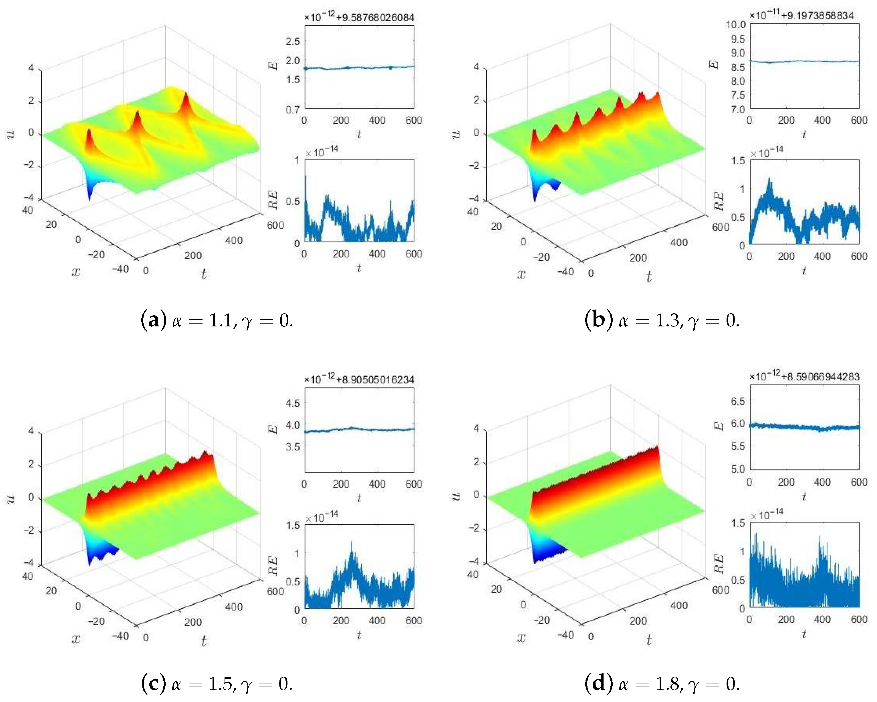
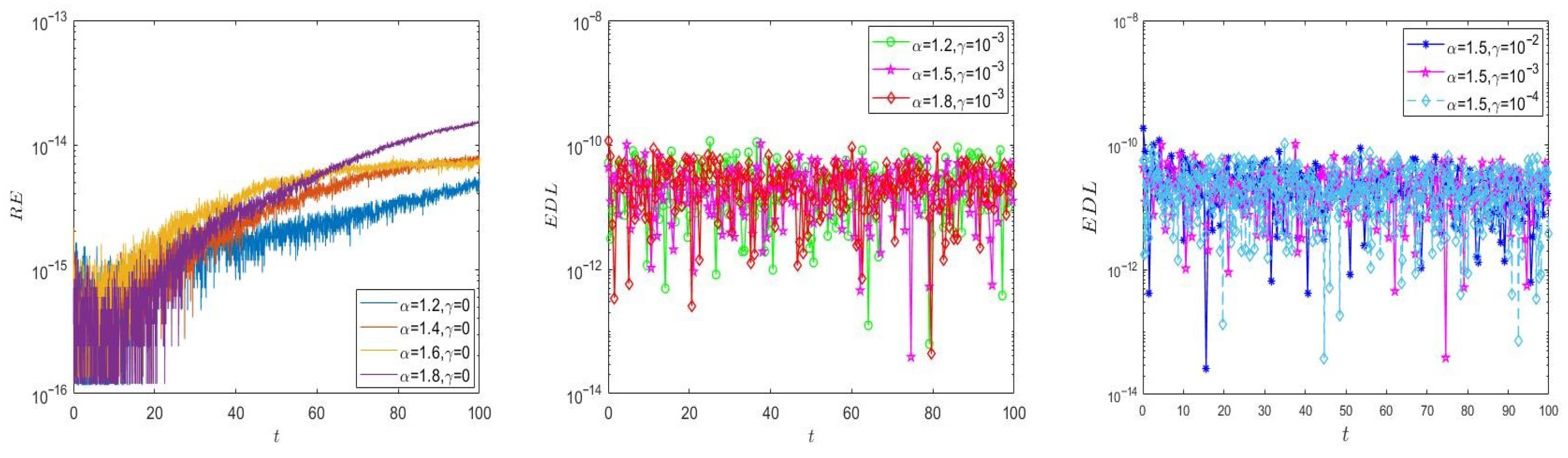
5.1. One-Dimensional Problem

Example 1

(Convergence Rate). The SAV-WSLD-Gauss method is used on the one-dimensional Riesz space fractional sine-Gordon equation [38]

$$\frac{{\partial }^{2}u(x,t)}{\partial t^2}-\frac{{\partial }^{\alpha }u(x,t)}{{\partial \left|x\right|}^{\alpha }}+\gamma \frac{\partial u(x,t)}{\partial t}+sin\left(u\right)=f(x,t),$$

(18)

on $\mathsf{\Omega }=(0,1)\times (0,1]$ with the forcing function

$$\begin{array}{cc}\hfill f(x,t)& =sin\left(exp(-t)x^4{(1-x)}^4\right)+(1-\gamma )exp(-t)x^4{(1-x)}^4\hfill \\ \hfill & +\frac{exp(-t)}{2cos(\alpha \pi /2)}[\mathsf{\Gamma }\left(5\right)\frac{x^{4-\alpha }+{\left(1-x\right)}^{4-\alpha }}{\mathsf{\Gamma }(5-\alpha )}-4\mathsf{\Gamma }\left(6\right)\frac{x^{5-\alpha }+{\left(1-x\right)}^{5-\alpha }}{\mathsf{\Gamma }(6-\alpha )}\hfill \\ \hfill & +6\mathsf{\Gamma }\left(7\right)\frac{x^{6-\alpha }+{\left(1-x\right)}^{6-\alpha }}{\mathsf{\Gamma }(7-\alpha )}-4\mathsf{\Gamma }\left(8\right)\frac{x^{7-\alpha }+{\left(1-x\right)}^{7-\alpha }}{\mathsf{\Gamma }(8-\alpha )}\hfill \\ \hfill & +\mathsf{\Gamma }\left(9\right)\frac{x^{8-\alpha }+{\left(1-x\right)}^{8-\alpha }}{\mathsf{\Gamma }(9-\alpha )}].\hfill \end{array}$$

The problem is subjected to the initial and boundary conditions

$$\begin{array}{cc}\hfill & u(x,0)=x^4{(1-x)}^4,\frac{\partial u(x,0)}{\partial t}=-x^4{(1-x)}^4,0<x<1,\hfill \\ \hfill & u(0,t)=u(1,t)=0,0<t\le 1.\hfill \end{array}$$

Under these conditions, the solution of (18) can be given as $u(x,t)=exp(-t)x^4{(1-x)}^4$.

The error of the numerical solutions at point $t=T$ is computed by

$$e(h,\tau )=\sqrt{h\sum _{i=1}^{N_x-1}{\left|u(x_i,T)-u_i^{N_t}\right|}^2},$$

which is in the sense of $l_2$-norm. The notation $e(h,\tau )$ means that the numerical error is defined relative to the step size h and τ. The EOC is measured by

$$EOC={log}_2\frac{e(h,\tau )}{e(h/2,\tau /2)}.$$

The numerical results presented in

Table 1. The errors and EOCs of SAV-WSLD-Gauss2 method for Equation (18) at time $T=1$ by keeping $h=\tau$.

$\mathit{\gamma }$	$\mathit{h}=\mathit{\tau }$	$\mathit{\alpha }=1.2$		$\mathit{\alpha }=1.5$		$\mathit{\alpha }=1.8$
		$\mathit{e}(\mathit{h},\mathit{\tau })$	EOC	$\mathit{e}(\mathit{h},\mathit{\tau })$	EOC	$\mathit{e}(\mathit{h},\mathit{\tau })$	EOC
0	1/32	$1.0360\times {10}^{-6}$	–	$1.5695\times {10}^{-6}$	–	$2.4488\times {10}^{-6}$	–
	1/64	$1.0202\times {10}^{-7}$	3.3440	$1.6704\times {10}^{-7}$	3.2321	$2.2301\times {10}^{-7}$	3.4569
	1/128	$1.0820\times {10}^{-8}$	3.2372	$1.2822\times {10}^{-8}$	3.7035	$1.8629\times {10}^{-8}$	3.5815
	1/256	$9.0514\times {10}^{-10}$	3.5794	$8.4072\times {10}^{-10}$	3.9308	$1.3073\times {10}^{-9}$	3.8328
	1/512	$6.5798\times {10}^{-11}$	3.7820	$4.9729\times {10}^{-11}$	4.0795	$8.7192\times {10}^{-11}$	3.9063
$0.5$	1/32	$9.3381\times {10}^{-7}$	–	$1.0533\times {10}^{-6}$	–	$2.2008\times {10}^{-6}$	–
	1/64	$8.8469\times {10}^{-8}$	3.3999	$1.1863\times {10}^{-7}$	3.1503	$1.8711\times {10}^{-7}$	3.5561
	1/128	$9.3011\times {10}^{-9}$	3.2497	$9.2250\times {10}^{-9}$	3.6848	$1.5164\times {10}^{-8}$	3.6252
	1/256	$7.7177\times {10}^{-10}$	3.5911	$6.0515\times {10}^{-10}$	3.9302	$1.0645\times {10}^{-9}$	3.8324
	1/512	$5.5373\times {10}^{-11}$	3.8009	$3.8726\times {10}^{-11}$	3.9659	$7.0728\times {10}^{-11}$	3.9118

show that the SAV-WSLD-Gauss2 scheme is fourth-order accurate in space and time directions with different α and γ.

Example 2

(Energy conservation or dissipation). In this test, the discrete energy conservation or dissipation properties of the proposed schemes will be shown through numerical experiments of system (1) by setting $F\left(u\right)=1-cos\left(u\right)$ on $\mathsf{\Omega }=(-40,40)\times (0,T]$. Here, we consider the fractional sine-Gordon equation with the initial value defined by the exact solution of the standard sine-Gordon equation (i.e., $\alpha =2$ and $\gamma =0$ for system (1)) as follows:

$$\begin{array}{c}\hfill \psi \left(x\right)=4arctan\left(\frac{\sqrt{1-{\omega }^2}}{\omega cosh\sqrt{1-{\omega }^2}x}\right),\varphi \left(x\right)=0,x\in [-40,40],\end{array}$$

with $0<\omega <1$. Since the exact solution of this example is unavailable, the error of the numerical solutions is measured by

$$E_{h,\tau }={\parallel U_{h,\tau }-U_{2h,2\tau }\parallel }_2,$$

in the sense of $l_2$-norm, where $U_{h,\tau }$ denotes the numerical solutions relative to the step size h and τ. Then, the EOC is measured by

$$EOC={log}_2\frac{E_{h,\tau }}{E_{h/2,\tau /2}}.$$

The numerical results in

Table 2. The errors and EOCs of SAV-WSLD-Gauss2 method for Example 2 with different $\alpha$ and $\gamma =0$ at time $T=1$ by keeping $h=\tau$.

$\mathit{h}=\mathit{\tau }$	$\mathit{\alpha }=1.2$		$\mathit{\alpha }=1.5$		$\mathit{\alpha }=1.8$
	${\mathit{E}}_{\mathit{h},\mathit{\tau }}$	EOC	${\mathit{E}}_{\mathit{h},\mathit{\tau }}$	EOC	${\mathit{E}}_{\mathit{h},\mathit{\tau }}$	EOC
1/4	$2.7999\times {10}^{-3}$	–	$1.0835\times {10}^{-3}$	–	$3.2993\times {10}^{-3}$	–
1/8	$8.0118\times {10}^{-5}$	5.1271	$2.5184\times {10}^{-4}$	2.1051	$4.1437\times {10}^{-4}$	2.9932
1/16	$2.6900\times {10}^{-5}$	1.5745	$2.1058\times {10}^{-5}$	3.5800	$3.0156\times {10}^{-5}$	3.7804
1/32	$5.7247\times {10}^{-6}$	2.2323	$1.4625\times {10}^{-6}$	3.8479	$1.9832\times {10}^{-6}$	3.9265
1/64	$1.7007\times {10}^{-6}$	1.7511	$7.0435\times {10}^{-7}$	1.0540	$1.5403\times {10}^{-7}$	3.6865

display the errors $E_{h,\tau }$ at $T=1$ and EOCs of the SAV-WSLD-Gauss2 scheme with different α and $\gamma =0$ for Example 2 on $\mathsf{\Omega }=(-40,40)\times (0,1]$. The lower regularity of the solutions for this example leads to a corresponding lower order of convergence.

Now, we use the SAV-WSLD-Gauss3 method to solve the fractional sine-Gordon equation with the space step $h=1/4$ and time step $\tau =1/16$ for different values of α and γ. When $\gamma =0$, the energy of system (1) is conservative. Figure 1 depicts the surfaces of the numerical solution $u_i^n$ of Example 2 computed by SAV-WSLD-Gauss3 in the left sub-figure. The discrete energy $E_n$ defined by (14) is shown in the upper right corner. The corresponding relative errors of the discrete energy $R{E}_n$ are defined by

$$R{E}_n={log}_{10}\frac{|E_n-E_0|}{|E_0|}.$$

For this example, the $R{E}_n$ is shown in the bottom right corner for $\gamma =0$ and different values of α in Figure 1.

It is obvious that the SAV-WSLD-Gauss scheme (13) is energy conserving for $\gamma =0$. Moreover, the impact of the different values of α on the surfaces of the numerical solutions can be seen in Figure 1 distinctly. It can be seen that the SAV-WSLD-Gauss methods are suitable for long-time simulations.

When $\gamma >0$, the energy of system (1) is dissipative. In this case, we plot the surfaces of the numerical solutions obtained by using SAV-WSLD-Gauss3 for different values of γ and α in Figure 2. To test the energy dissipation law of SAV-WSLD-Gauss methods, we define the error in the discrete dissipation-preserving law $ED{L}_n$ as

$$\begin{array}{c}\hfill ED{L}_n=\left|{\delta }_t{E}_n+\gamma {∥v^n∥}_2^2\right|,p\le n\le N_t-p,\end{array}$$

(19)

where ${\delta }_t{E}_n$ denotes the derivative of the energy, which is calculated by using a five-point scheme and Richardson extrapolation from $E_n$, and p is determined by the time extrapolation. The values of $v^n$ can be obtained in the process of the numerical calculation. The discrete energy $E_n$ and the error in discrete dissipation-preserving law $ED{L}_n$ are shown graphically in the right sub-figure of Figure 2.

Since the derivative of energy is approximated by numerical methods with an eighth-order accuracy, the error of the discrete dissipation-preserving law $ED{L}_n$ is caused by the truncation error of the numerical derivative of energy in a certain degree. However, the $ED{L}_n$ indicated in Figure 2 can still reach ${10}^{-12}$ for the time step $\tau =1/32$. The results show that the energy of the numerical schemes approximately follows the energy dissipative law of the continuous equations for the case $\gamma >0$. The numerical results are consistent with the conclusion of Theorem 4.

Besides, the surfaces of the numerical solutions with various γ are described in Figure 2. The numerical results show that the amplitude of solutions tends to decrease with reduced γ. Moreover, the dispersive effects of the parameter γ can also be observed in Figure 2. The smaller the values of γ, the smaller the rate of change of the discrete energy.

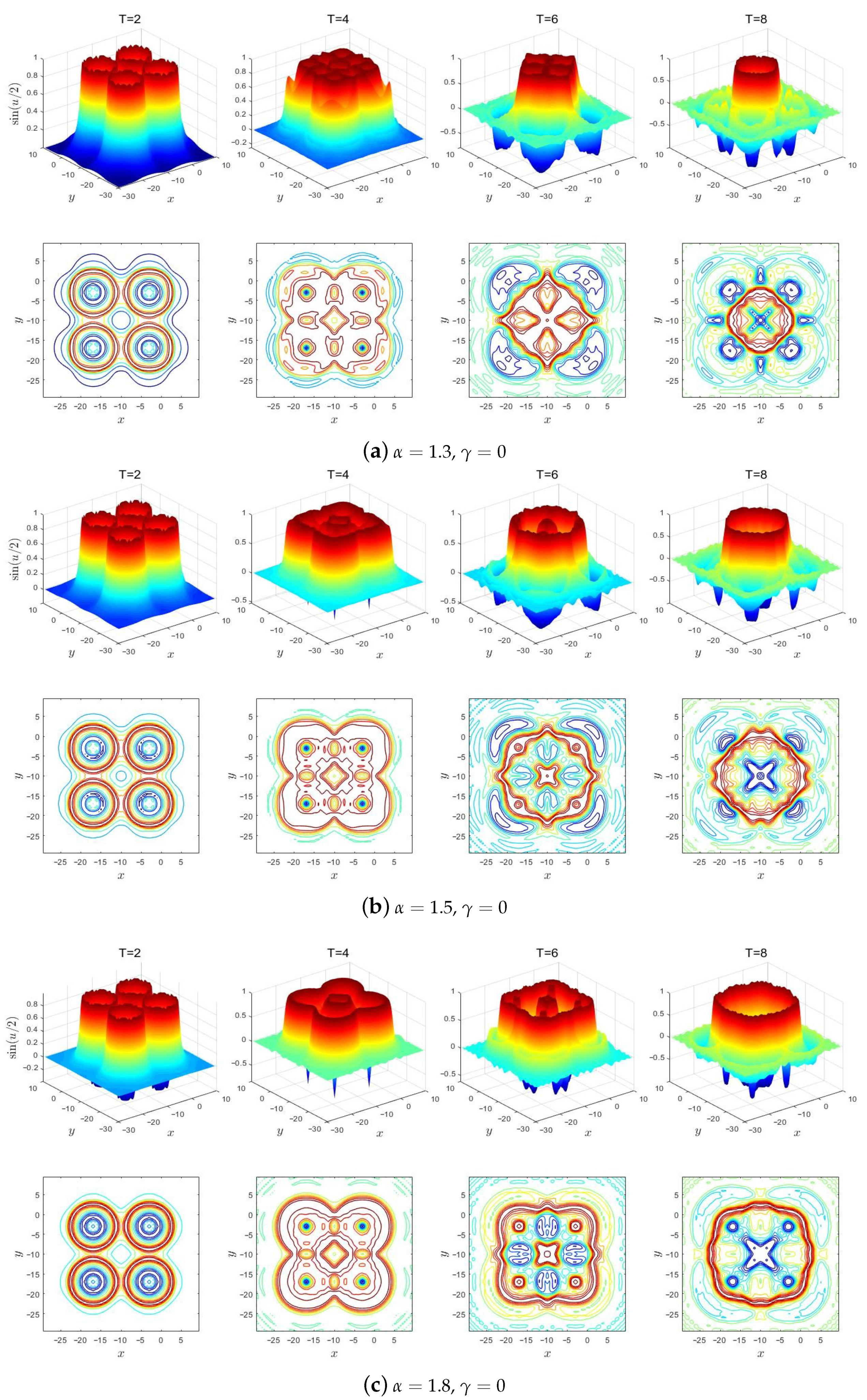
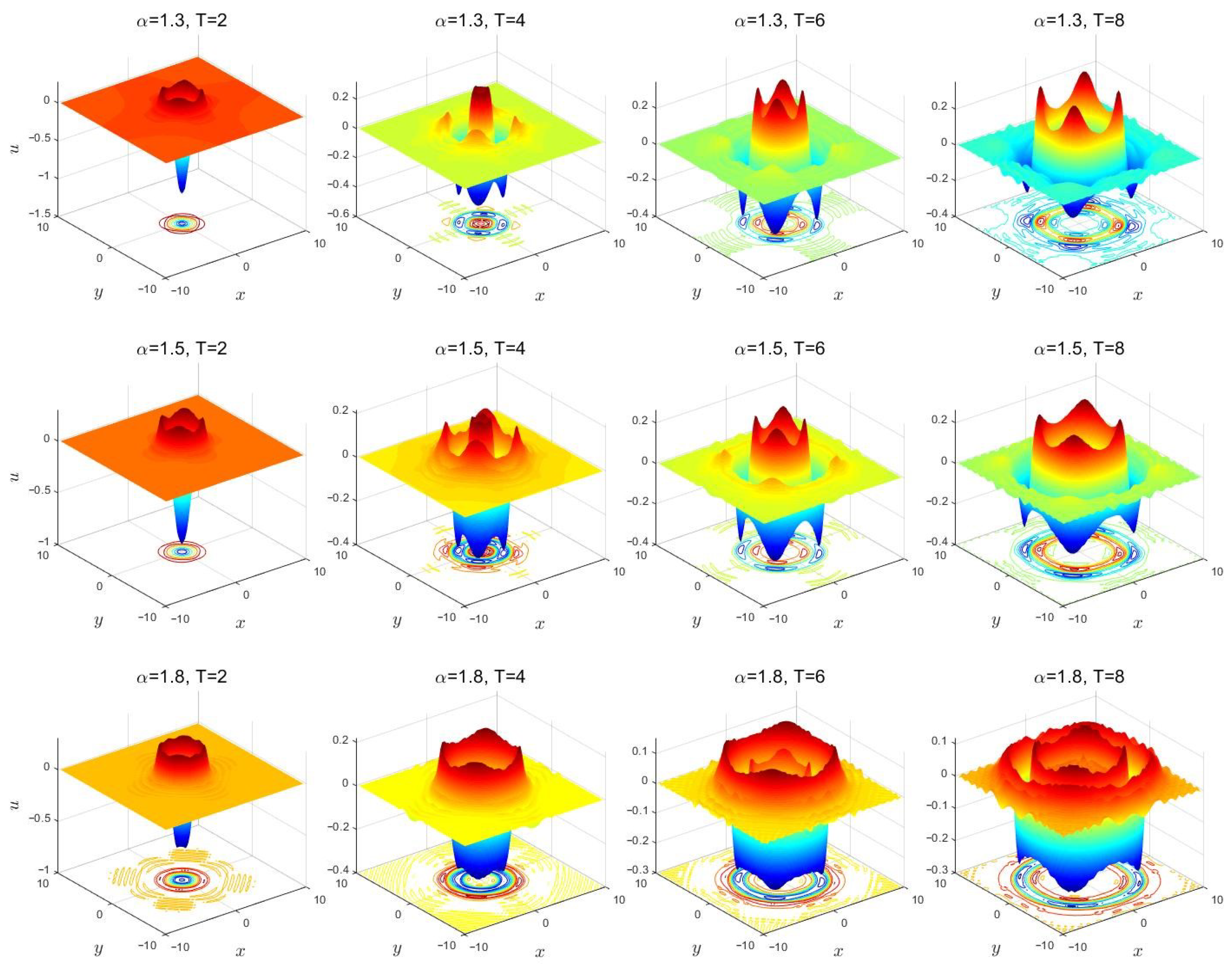
5.2. Two-Dimensional Problem

Example 3.

We use the SAV-WSLD-Gauss methods on system (16) with function $F\left(u\right)=1-cos\left(u\right)$ in two space dimensions on $(-30,10)\times (-30,10)\times (0,T]$. The initial values are given as

$$\begin{array}{c}\hfill \psi (x,y)=4\sum _{i=0}^1\sum _{j=0}^{1}arctan\left[exp\left(\frac{4-\sqrt{{(x+3+14i)}^2+{(y+3+14j)}^2}}{0.436}\right)\right],\end{array}$$

and the boundary values are given as

$$\begin{array}{c}\hfill \varphi (x,y)=4.13\sum _{i=0}^1\sum _{j=0}^1\frac{1}{cosh\left[\left(4-\sqrt{{(x+3+14i)}^2+{(y+3+14j)}^2}\right)/0.436\right]}.\end{array}$$

We use the SAV-WSLD-Gauss3 method to solve this problem by setting $h_x=h_y=1/2$ and $\tau =1/4$.

To consider the case of the collision of four ring solitons within the framework of the fractional sine-Gordon equation, we show the numerical solutions in terms of $sin(u/2)$ at different time T and the related contour of Example 3 in Figure 3 for $\alpha =1.3,1.5,1.8$, respectively. In Figure 3, we investigate the impact of the Riesz fractional order α on the surface evolution. These figures correctly characterize the collision of four expanding circular ring solitons. Moreover, they reflect the complex interaction with distinctly altering values of u in the center of the collision. These results coincide with the conclusions proposed in [39,40].

In Figure 4, we present the energy errors $R{E}_n$ for different α and $\gamma =0$ of Example 3 on domain $(-5,5)\times (-5,5)$ within a relatively long time $t\in (0,100]$ with $h_x=h_y=1/2$ and $\tau =0.01$. Obviously, our scheme can conserve the energy very well in long-time integration. The efficiency of the SAV-WSLD-Gauss scheme is also verified. To verify the dissipation-preserving law of the present methods, the $ED{L}_n$ are also shown for different α and γ. The dissipation-preserving law of Example 3 is also conserved by the present numerical method.

Example 4.

We use the SAV-WSLD-Gauss methods on system (16) with function $F\left(u\right)=u^4/4$ in two space dimensions on $(-10,10)\times (-10,10)\times (0,T]$. The boundary and initial conditions are given as

$$\begin{array}{c}\hfill \psi (x,y)=\frac{2}{cosh\left[cosh\left(x^2+y^2\right)\right]},\varphi (x,y)=0.\end{array}$$

We use the SAV-WSLD-Gauss3 method to solve this two-dimensional problem by setting $h_x=h_y=1/4$ and $\tau =1/16$. The surface of the numerical solutions and the corresponding contour of Example 4 for $\alpha =1.3,1.5$ and $1.8$ at different times T are shown in Figure 5. The solutions of the two-dimensional space fractional Klein–Gordon equations appear to follow a periodic behavior. Moreover, from these figures, we can see the radiation, shrink, and oscillation of the circular ring solitons, together with the expansion and propagation of the initial soliton to the whole domain before they get the boundary. It also can be seen that the order of the Riesz fractional derivative α affects the forms of the circular ring soliton. The speed at which solitons reach the boundary is faster for bigger α. The numerical results coincide with the corresponding surface given in the literature [38].

In Figure 6, we present the relative energy errors $R{E}_n$ over a long time for different α and $\gamma =0$ of Example 4 on domain $(-5,5)\times (-5,5)\times (0,100]$ with $h_x=h_y=1/4$ and $\tau =0.01$, and the $ED{L}_n$ for several γ and α. It can be seen that $R{E}_n$ and $ED{L}_n$ roughly reach the machine accuracy, which implies that the energy or dissipation-preserving law of Example 4 is conserved well by the present numerical method.

6. Conclusions

This paper developed and analyzed a class of high-order dissipation-preserving methods for nonlinear fractional generalized wave equations based on the SAV approach, in which the time and space are discretized by a fourth-order preserving approximation and the collocation methods, respectively. The proposed scheme can achieve fourth-order accuracy in space and arbitrarily high-order accuracy in time. The unconditional energy or dissipation conservation of the schemes was proved strictly. Finally, the theoretical results are verified by some numerical experiments.

References

1. Kilbas, A.A.; Srivastava, H.M.; Trujillo, J.J. Theory and Applications of Fractional Differential Equations; Elsevier: Amsterdam, The Netherlands, 2006; Volume 204. [Google Scholar]
2. Baleanu, D.; Diethelm, K.; Scalas, E.; Trujillo, J.J. Fractional Calculus: Models and Numerical Methods; World Scientific: Singapore, 2012; Volume 3. [Google Scholar]
3. Gu, X.M.; Zhao, Y.L.; Zhao, X.L.; Carpentieri, B.; Huang, Y.Y. A note on parallel preconditioning for the all-at-once solution of Riesz fractional diffusion equations. Numer. Math. Theor. Meth. Appl. 2021, 14, 893–919. [Google Scholar]
4. Zhao, J.; Jiang, X.; Xu, Y. A kind of generalized backward differentiation formulae for solving fractional differential equations. Appl. Math. Comput. 2022, 419, 126872. [Google Scholar] [CrossRef]
5. Tarasov, V.E. Continuous limit of discrete systems with long-range interaction. J. Phys. A Math. Gen. 2006, 39, 14895. [Google Scholar] [CrossRef] [Green Version]
6. Campa, A.; Dauxois, T.; Ruffo, S. Statistical mechanics and dynamics of solvable models with long-range interactions. Phys. Rep. 2009, 480, 57–159. [Google Scholar] [CrossRef] [Green Version]
7. Wang, N.; Li, M.; Huang, C. Unconditional energy dissipation and error estimates of the SAV Fourier spectral method for nonlinear fractional generalized wave equation. J. Sci. Comput. 2021, 88, 1–32. [Google Scholar] [CrossRef]
8. Huang, Y.Y.; Gu, X.M.; Gong, Y.; Li, H.; Zhao, Y.L.; Carpentieri, B. A fast preconditioned semi-implicit difference scheme for strongly nonlinear space-fractional diffusion equations. Fractal Fract. 2021, 5, 230. [Google Scholar] [CrossRef]
9. Macías-Díaz, J. A numerically efficient dissipation-preserving implicit method for a nonlinear multidimensional fractional wave equation. J. Sci. Comput. 2018, 77, 1–26. [Google Scholar] [CrossRef]
10. Scherer, R.; Kalla, S.L.; Tang, Y. The Grünwald-Letnikov method for fractional differential equations. Comput. Math. Appl. 2011, 62, 902–917. [Google Scholar] [CrossRef] [Green Version]
11. Hao, Z.; Sun, Z.; Cao, W. A fourth-order approximation of fractional derivatives with its applications. J. Comput. Phys. 2015, 281, 787–805. [Google Scholar] [CrossRef]
12. Diethelm, K.; Ford, N.J.; Freed, A.D. Detailed error analysis for a fractional Adams method. Numer. Algorithms 2004, 36, 31–52. [Google Scholar] [CrossRef] [Green Version]
13. Chen, M.; Deng, W. Fourth order accurate scheme for the space fractional diffusion equations. SIAM J. Numer. Anal. 2014, 52, 1418–1438. [Google Scholar] [CrossRef] [Green Version]
14. Fu, Y.; Cai, W.; Wang, Y. A linearly implicit structure-preserving scheme for the fractional sine-Gordon equation based on the IEQ approach. Appl. Numer. Math. 2021, 160, 368–385. [Google Scholar] [CrossRef]
15. Macías-Díaz, J. An explicit dissipation-preserving method for Riesz space-fractional nonlinear wave equations in multiple dimensions. Commun. Nonlinear Sci. Numer. Simul. 2018, 59, 67–87. [Google Scholar] [CrossRef]
16. Zhao, J.; Li, Y.; Xu, Y. An explicit fourth-order energy-preserving scheme for Riesz space fractional nonlinear wave equations. Appl. Math. Comput. 2019, 351, 124–138. [Google Scholar] [CrossRef]
17. Serna-Reyes, A.J.; Macías-Díaz, J.E. A mass-and energy-conserving numerical model for a fractional Gross–Pitaevskii system in multiple dimensions. Mathematics 2021, 9, 1765. [Google Scholar] [CrossRef]
18. Fu, Y.; Cai, W.; Wang, Y. An explicit structure-preserving algorithm for the nonlinear fractional Hamiltonian wave equation. Appl. Math. Lett. 2020, 102, 106123. [Google Scholar] [CrossRef]
19. Xie, J.; Zhang, Z. An effective dissipation-preserving fourth-order difference solver for fractional in space nonlinear wave equations. J. Sci. Comput. 2019, 79, 1753–1776. [Google Scholar] [CrossRef]
20. Xie, J.; Zhang, Z.; Liang, D. A new fourth-order energy dissipative difference method for high-dimensional nonlinear fractional generalized wave equations. Commun. Nonlinear Sci. Numer. Simul. 2019, 78, 104850. [Google Scholar] [CrossRef]
21. Li, M.; Fei, M.; Wang, N.; Huang, C. A dissipation-preserving finite element method for nonlinear fractional wave equations on irregular convex domains. Math. Comput. Simul. 2020, 177, 404–419. [Google Scholar] [CrossRef]
22. Kang, M.; You, D. A low dissipative and stable cell-centered finite volume method with the simultaneous approximation term for compressible turbulent flows. Mathematics 2021, 9, 1206. [Google Scholar] [CrossRef]
23. Wang, N.; Shi, D. Two efficient spectral methods for the nonlinear fractional wave equation in unbounded domain. Math. Comput. Simul. 2021, 185, 696–718. [Google Scholar] [CrossRef]
24. Shen, J.; Xu, J.; Yang, J. The scalar auxiliary variable (SAV) approach for gradient flows. J. Comput. Phys. 2018, 353, 407–416. [Google Scholar] [CrossRef]
25. Huang, F.; Shen, J.; Yang, Z. A highly efficient and accurate new scalar auxiliary variable approach for gradient flows. SIAM J. Sci. Comput. 2020, 42, A2514–A2536. [Google Scholar] [CrossRef]
26. Fu, Y.; Hu, D.; Wang, Y. High-order structure-preserving algorithms for the multi-dimensional fractional nonlinear Schrödinger equation based on the SAV approach. Math. Comput. Simul. 2021, 185, 238–255. [Google Scholar] [CrossRef]
27. Cui, J.; Xu, Z.; Wang, Y.; Jiang, C. Mass and energy-preserving exponential Runge-Kutta methods for the nonlinear Schrödinger equation. Appl. Math. Lett. 2021, 112, 106770. [Google Scholar] [CrossRef]
28. Li, X.; Gong, Y.; Zhang, L. Linear high-Order energy-preserving schemes for the nonlinear schrödinger equation with wave operator using the scalar auxiliary variable approach. J. Sci. Comput. 2021, 88, 1–25. [Google Scholar] [CrossRef]
29. Huang, Q.; Zhang, G.; Wu, B. Fully-discrete energy-preserving scheme for the space-fractional Klein-Gordon equation via Lagrange multiplier type scalar auxiliary variable approach. Math. Comput. Simul. 2022, 192, 265–277. [Google Scholar] [CrossRef]
30. Hendy, A.S.; Macías-Díaz, J. On a nonlinear energy-conserving scalar auxiliary variable (SAV) model for Riesz space-fractional hyperbolic equations. Appl. Numer. Math. 2021, 165, 339–347. [Google Scholar] [CrossRef]
31. Lischke, A.; Pang, G.; Gulian, M. What is the fractional Laplacian? A comparative review with new results. J. Comput. Phys. 2020, 404, 109009. [Google Scholar] [CrossRef]
32. Yang, Q.; Liu, F.; Turner, I. Numerical methods for fractional partial differential equations with Riesz space fractional derivatives. Appl. Mathe. Model. 2010, 34, 200–218. [Google Scholar] [CrossRef] [Green Version]
33. Vong, S.; Wang, Z. A compact difference scheme for a two dimensional fractional Klein-Gordon equation with Neumann boundary conditions. J. Comput. Phys. 2014, 274, 268–282. [Google Scholar] [CrossRef]
34. Chen, S.; Jiang, X.; Liu, F.; Turner, I. High order unconditionally stable difference schemes for the Riesz space-fractional telegraph equation. J. Comput. Appl. Math. 2015, 278, 119–129. [Google Scholar] [CrossRef] [Green Version]
35. Leimkuhler, B.; Reich, S. Simulating Hamiltonian Dynamics; Number 14; Cambridge University Press: Cambridge, UK, 2004. [Google Scholar]
36. Hairer, E.; Lubich, C.; Wanner, G. Geometric Numerical Integration: Structure-Preserving Algorithms for Ordinary Differential Equations; Springer Science & Business Media: Berlin/Heidelberg, Germany, 2006; Volume 31. [Google Scholar]
37. Wang, P.; Huang, C. An implicit midpoint difference scheme for the fractional Ginzburg-Landau equation. J. Comput. Phys. 2016, 312, 31–49. [Google Scholar] [CrossRef] [Green Version]
38. Hu, D.; Cai, W.; Song, Y.; Wang, Y. A fourth-order dissipation-preserving algorithm with fast implementation for space fractional nonlinear damped wave equations. Commun. Nonlinear Sci. Numer. Simul. 2020, 91, 105432. [Google Scholar] [CrossRef]
39. Xing, Z.; Wen, L.; Wang, W. An explicit fourth-order energy-preserving difference scheme for the Riesz space-fractional sine-Gordon equations. Math. Comput. Simul. 2021, 181, 624–641. [Google Scholar] [CrossRef]
40. Jiang, C.; Cai, W.; Wang, Y. A linearly implicit and local energy-preserving scheme for the sine-Gordon equation based on the invariant energy quadratization approach. J. Sci. Comput. 2019, 80, 1629–1655. [Google Scholar] [CrossRef] [Green Version]
Figure 1. Surfaces of numerical solution, the discrete energy E n , and the relative errors of the discrete energy R E n for γ = 0 and different α with h = 1 / 4 and τ = 1 / 16 .
Fractalfract 06 00264 g001
Figure 2. Surfaces of the numerical solutions, discrete energy E n , and the discrete dissipation-preserving law E D L n for different α and γ with h = 1 / 4 and τ = 1 / 32 .
Fractalfract 06 00264 g002
Figure 3. The numerical solutions in terms of sin ( u / 2 ) and contour at different time T for different α with h = 1 / 2 , τ = 1 / 4 .
Fractalfract 06 00264 g003
Figure 4. The relative energy errors R E n for γ = 0 and the errors in discrete dissipation-preserving law E D L n for different γ and α with h x = h y = 1 / 2 and τ = 0.01 .
Fractalfract 06 00264 g004
Figure 5. Surfaces of the numerical solutions and contour of Example 4 at time T with h x = h y = 1 / 4 , τ = 1 / 16 for γ = 0 and different α .
Fractalfract 06 00264 g005
Figure 6. The relative energy errors R E n for γ = 0 and the errors in discrete dissipation-preserving law E D L n for different γ and α with h x = h y = 1 / 4 and τ = 0.01 .
Fractalfract 06 00264 g006