Article

Image Dehazing Based on Local and Non-Local Features

1
School of Optics and Photonics, Beijing Institute of Technology, Beijing 100081, China
2
Beijing Key Laboratory for Precision Optoelectronic Measurement Instrument and Technology, School of Optics and Photonics, Beijing Institute of Technology, Beijing 100081, China
3
Intelligent Sensing Innovation Research Center, Yangtze Delta Region Academy of Beijing Institute of Technology, Jiaxing 314019, China
*
Author to whom correspondence should be addressed.
Fractal Fract. 2022, 6(5), 262; https://doi.org/10.3390/fractalfract6050262
Submission received: 29 March 2022 / Revised: 1 May 2022 / Accepted: 5 May 2022 / Published: 9 May 2022

Abstract

:
Image dehazing is a traditional task, yet it still presents arduous problems, especially in the removal of haze from the texture and edge information of an image. The state-of-the-art dehazing methods may result in the loss of some visual informative details and a decrease in visual quality. To improve dehazing quality, a novel dehazing model is proposed, based on a fractional derivative and data-driven regularization terms. In this model, the contrast constrained adaptive histogram equalization method is used as the data fidelity item; the fractional derivative is applied to avoid over-enhancement and noise amplification; and the proposed data-driven regularization terms are adopted to extract the local and non-local features of an image. Then, to solve the proposed model, half-quadratic splitting is used. Moreover, a dual-stream network based on Convolutional Neural Network (CNN) and Transformer is introduced to structure the data-driven regularization. Further, to estimate the atmospheric light, an atmospheric light model based on the fractional derivative and the atmospheric veil is proposed. Extensive experiments display the effectiveness of the proposed method, which surpasses the state-of-the-art methods for most synthetic and real-world images, quantitatively and qualitatively.

1. Introduction

Single-image dehazing is one of the most classical and fundamental non-linear inverse problems in image processing, which aims to estimate high-quality images from hazy ones. Because light is scattered and absorbed as the distance from an image increases, particularly in bad weather, dehazing equipment or method may be required. To reduce the impact of haze and to accurately estimate high-quality images, single-image haze removal is a vital pre-processing step in removing haze and thin clouds from haze-affected images. To quantitatively measure the effect of haze on an image, many single-image dehazing algorithms are based on the dichromatic model. This model describes a hazy image as a mixture of the transmitted portion of the ideal image and the portion of the light source that reaches the optical imaging equipment. Mathematically, the hazy image formation [1] model can be written in the form of Equation (1):
I = J t + A ( 1 t )
where I is the observed image in bad weather, J is the ideal image, A is the air-light, and t is the transmission map. From Equation (1), the transmission map t plays a core role in determining the clarity of a restored image. As the atmospheric light vector A is unknown, the accurate estimation of the transmission map t is a challenging problem.
Generally, the estimation of t is divided into two stages: a rough transmission map, and a refined transmission map. The rough t can be estimated via imaging model-based methods, including Dark Channel Prior (DCP) [2], Hazy-Line Prior (HLP) [3], or Color Attenuation Prior (CAP) [4]. However, the refined t is difficult to estimate, and it plays a key role in image restoration, because t can provide edge and texture information to image restoration in bad weather.
During the past decade, the guide filter [5] method is the most well-known; it transfers the structures and textures of the guidance image to the output image. Based on the guide filter, the weighted guided image filter [6], the gradient-domain guided image filter [7], and the anisotropic guided filtering method [8] have been widely employed in image dehazing, due to their low complexity and good edge-preservation properties. In addition, the total variation (TV) prior process [9] is a prominent regularization tool for estimating t, because the TV prior helps in preserving the sharp edges and textures of an image and prevents solutions from having oscillations. Therefore, numerous TV-based methods have been proposed for use in hazy weather. Bredies et al. [10] proposed the concept of total generalized variation (TGV) of a function without producing staircasing effects. Gilboa et al. [11] applied a complex diffusion process by using the Schrodinger equation. A linear solution was obtained for the complex diffusion process, which could estimate a high-quality restored image. Recently, Liu et al. [12] estimated the refined t by using non-local total variation regularization. Jiao et al. [13] proposed a hybrid model, with first- and second-order variations, and they improved the hybrid model via adaptive parameters. Parisotto et al. [14] introduced higher-order anisotropic total variation regularization, and used a primal-dual hybrid gradient approach to approximate numerically the associated gradient flow. However, the TV-based methods suffer from two defects: a staircasing effect, and a non-convex and non-smooth term. Fortunately, fractional-order calculus [15] may be a powerful tool to alleviate these problems.
Fractional-order calculus is a generalization of integer-order calculus, which has provided for great advances in image processing. Chan et al. [16] applied spatially adaptive fractional-order diffusion to restore images. Svynchuk et al. [17] studied remote sensing image compression by using fractal functions. Zhang et al. [18] proposed image enhancement based on particle swarm optimization and an adaptive fractional differential filter. Xu et al. [19] improved the scale-invariant feature transform via an adaptive fractional differential dynamic mask. Luo et al. [20] demonstrated that a fractional differential operator is capable of enhanced performance, superior to that of integral differential operators in remote sensing images. Fang et al. proposed a nonlinear gradient domain-guided filtering method for image dehazing, which was optimized via a fractional-order gradient descent with momentum for the RBF neural network. In addition, the above estimation methods have two problems to be solved. One problem is the incorrect estimation of the infinite depth of field; this problem can be ameliorated via segmentation technology [21,22,23,24]. The other problem is error accumulation or amplification during multiple stages. For example, the DCP (HLP)-based methods include several steps, such as prior realization (dark channel or haze line), atmospheric light estimation, initial transmission, refined transmission, and image restoration. Due to the rapid development of deep learning technology, this second problem is disregarded, because the single-stage end-to-end model also can obtain high-quality images.
Since deep learning-based methods [25] have demonstrated prevailing success in image processing, the deep learning framework has been introduced to image dehazing. Zhou et al. [26] designed an end-to-end network based on the attention feature fusion module. Sun et al. [27] applied the cycle-consistent adversarial network, which was embedded in an iterative dehazing model. Zhang et al. [28] proposed a residual convolutional dehazing network, consisting of two subnetworks. Li et al. [29] proposed a novel dehazing method based on an unsupervised method, avoiding the strenuous labor of capturing hazy-clean image pairs. Golts et al. [30] also introduced an unsupervised dehazing method via minimization of the proposed DCP energy function. These deep learning-based methods can estimate high-quality images. Unfortunately, deep learning-based methods lack interpretability and physical significance, which limits their further development.
Although the above state-of-the-art methods achieve progress in image dehazing, we still find some problems: First, the physical prior-based methods are not well combined with deep learning-based methods, which make the deep learning-based methods learn image features aimlessly and without interpretability. Second, we regard the fractional differential as a powerful tool to further extract the mathematic prior, which can enhance the image quality in image dehazing and prevent image over-enhancement. Third, the problems of error accumulation and amplification of imaging model-based methods also need to be alleviated. Therefore, in this paper, we propose an image dehazing method based on the fractional differential and deep learning.
The main contributions of this paper are the following:
First, we propose a data-driven regularization term that includes local and non-local information about images. This regularization term can embed the physical model, which can constrain the aimlessness of the deep learning method. Moreover, the proposed regularization term can be regarded as a multi-scale fusion term (the small scale is for local information, and the large scale is for non-local information). Unlike the traditional multi-scale fusion method, the proposed method obtains the multi-scale information via data-driven information and big data instead of via image decomposition, as in a wavelet transform.
Second, we propose an image dehazing model based on the hazy imaging model, the fractional variation, and the above data-driven regularization term. The hazy imaging model can improve the physical significance for a data-driven regularization term and prevent the aimless learning of deep learning-based methods. The fractional variation can provide the mathematical feature for the proposed model and prevent over-enhancement and noise amplification. The data-driven regularization term can estimate the non-physical significance feature, which is highly abstract and nonlinear, to improve dehazing quality. Therefore, the proposed model is a deep learning-based method with physical significance and a mathematical feature.
Third, we unroll the proposed dehazing model into an unconstrained model. A novel network model, a Convolutional Neural Network (CNN) and a Swin Transformer, is proposed and used to solve local and non-local data-driven regularization terms, respectively. The architecture of the proposed network is intuitively interpretable by explicitly characterizing the local and non-local features and the hazy imaging model.
Finally, an atmospheric light estimation model is proposed, based on the atmospheric veil and the fractional variation, and this model is embedded in the above proposed dehazing method. Thus, the proposed model can be regarded as an end-to-end model, rather than as a multi-stage method, which can reduce the accumulation and amplification of errors during different stages.
The novel dehazing method is proposed via combining the technical contributions stated above. The remainder of this paper is structured as follows: Section 2 describes the proposed method and its basics. In Section 3, a series of experiments, including synthetic images and real-world images, are carried out to evaluate the presented method, qualitatively and quantitatively. Finally, Section 4 states conclusions about the proposed method. In addition, the Appendix A elaborates on each parameter in this paper.

2. Materials and Methods

The proposed dehazing method is an end-to-end (single stage) model combining the physical imaging model, the fractional derivative calculation, and deep learning. On the one hand, physical significance and mathematical features are helpful for the proposed network model in learning image features purposefully. On the other hand, the high-dimensional and nonlinear features extracted by deep learning models are effective supplements to the physical model and the mathematical prior.
In this section, the proposed dehazing method is discussed in detail. First, the fractional derivative is introduced in Section 2.1, which is the basic component of the proposed method. Then, a novel dehazing model is proposed in Section 2.2, and to solve this model, it is split into four subproblems. The data-driven regularization term-based subproblem is solved via the proposed network, which is introduced in Section 2.3. The other subproblems are solved in Section 2.4. The atmospheric light, which is an important component of image dehazing, is solved in Section 2.5. Finally, the pseudocode of our proposed method is displayed in Section 2.6.

2.1. Fractional Derivative

Several definitions of the fractional derivative were proposed in previous work, such as the Riemann-Liouville, the Grunwald-Letnikov, the Weyl, and the Caputo fractional derivatives. In this paper, the proposed method containing the fractional differential is formulated in terms of the left Riemann-Liouville derivative of order α, defined as in [31]
D x α f ( i , j ) = 1 Γ ( m α ) ( d d x ) m a i f ( τ , j ) ( i τ ) m α 1 d τ D y α f ( i , j ) = 1 Γ ( m α ) ( d d y ) m a j f ( τ , j ) ( j τ ) m α 1 d τ
where m is a positive integer, Γ is the Gamma function, f is a scalar function that is the image in this paper, i and j are the pixel coordinates of the image, and x and y are the horizontal and vertical directions, respectively. When α is a positive number, Equation (2) becomes the integer-order derivative. To reduce computational complexity, the standard discretization technique and the first-degree compound quadrature formula [32] were applied to the Riemann-Liouville operator:
D x α f ( i , j ) k = 0 m Ψ α ( k ) f ( i k , j ) , i = m + 1 , m + 2 , , M ; j = m + 1 , m + 2 , , N D y α f ( i , j ) k = 0 m Ψ α ( k ) f ( i , j k ) , i = m + 1 , m + 2 , , M ; j = m + 1 , m + 2 , , N
Ψ α ( k ) = ( 1 ) k Γ ( α + 1 ) k ! Γ ( α + 1 k ) ,
where k is the grid size of the standard discretization technique, m is a positive integer less than min (i, j), and m is the number of grids of the standard discretization technique. Equation (3) provides the vertical and horizontal directions of the discrete fractional-order derivatives of a hazy image, whose size is M × N at pixel position (i, j). The derivation process of discrete error in Equation (3) can be found in [33]. Analogously, the vertical and horizontal directions of the discrete right fractional-order derivatives can be defined as
( D x α ) * f ( i , j ) k = 0 m Ψ α ( k ) f ( i + k , j ) , i = 1 , 2 , , M m ; j = 1 , 2 , , N m ( D y α ) * f ( i , j ) k = 0 m Ψ α ( k ) f ( i , j + k ) , i = 1 , 2 , , M m ; j = 1 , 2 , , N m
To obtain multi-directions information, which can improve the quality of the dehazing result, the composite operator comprising right and left Riemann-Liouville operators was applied in the proposed method. It can be described as follows:
( D x α ) * D x α f ( i , j ) k = i m Ψ α ( k i ) p = 0 k Ψ α ( p ) f ( k p , j ) , i = m + 1 , m + 2 , , M m ; j = m + 1 , m + 2 , , N m ( D y α ) * D y α f ( i , j ) k = j m Ψ α ( k j ) p = 0 k Ψ α ( p ) f ( i , k p ) . i = m + 1 , m + 2 , , M m ; j = m + 1 , m + 2 , , N m

2.2. Proposed Dehazing Model
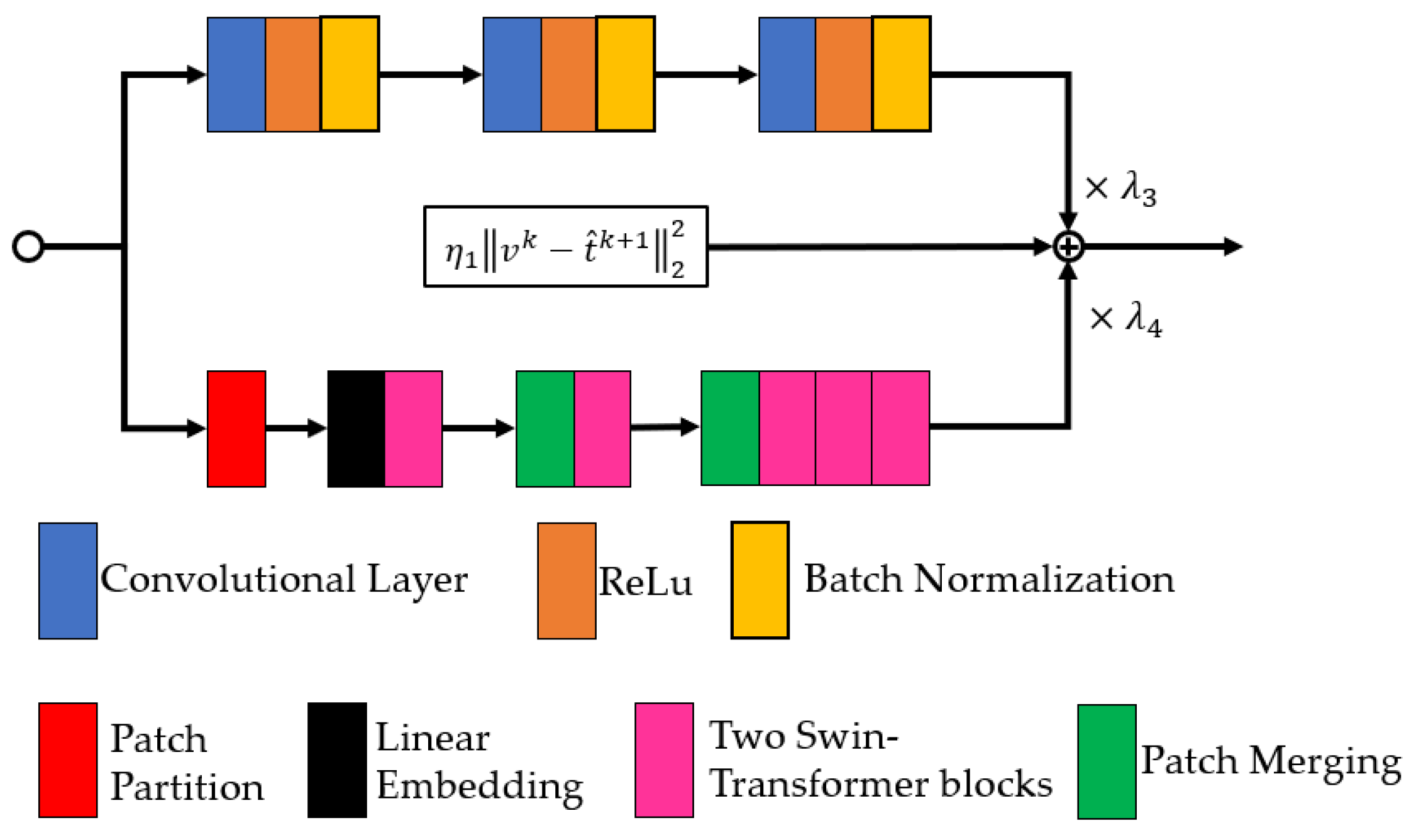
According to Equation (1), the proposed dehazing model based on optical imaging model is
( t ^ , J ^ ) = arg min t ^ , J ^ J ^ t ^ ( I A + A t ^ ) 2 2 + λ 1 2 I C L A H E J ^ 2 2 + λ 2 2 D α t ^ 1 + λ 3 C ( t ^ ) + λ 4 T ( t ^ )
where ICLAHE is the hazy image that has been enhanced via contrast-restricted histogram equalization (CLAHE) [34], and C ( · ) and T ( · ) are the local and non-local information regularization terms, respectively. λ1, λ2, λ3, and λ4 are the regularization parameters, which are positive numbers. D α is the fractional-order operator, D α = [ ( D x α ) * D x α , ( D y α ) * D y α ] T .   t ^ and J ^ are the transmission map and the ideal image to be optimized. | · | 1 and | · | 2 are the 1-norm and 2-norm operators. Both the first term and the second term are original image data fidelity items. The difference is that the first term can restore the background of the image and prevent image over-enhancement, while the second term focuses on restoring the texture and detail. The third, fourth, and fifth terms are the regularization terms.
Generally, the optimization problem, such as that shown in Equation (7), cannot be resolved directly; the solving strategy of proposed Equation (7) is to decouple Equation (7) into multiple subproblems. By adding the auxiliary valuables, Equation (7) can be written as a constrained optimization problem:
( t ^ , J ^ , v , w ) = arg min t ^ , J ^ , v , w J ^ t ^ ( I A + A t ^ ) 2 2 + λ 1 2 I C L A H E J ^ 2 2 + λ 2 2 w 1 + λ 3 C ( v ) + λ 4 T ( v ) , s . t . v = t ^ , w = D α t ^
Then, the half quadratic splitting (HQS) method, which has been widely used in image dehazing [35], image recovery [36], and super-resolution reconstruction [37], was applied to convert the above constrained optimization problem, as shown in Equation (8), to a non-constrained optimization problem:
( t ^ , J ^ , v , w ) = arg min t ^ , J ^ , v , w J ^ t ^ ( I A + A t ^ ) 2 2 + λ 1 2 I C L A H E J ^ 2 2   + λ 2 w 1 + λ 3 C ( v ) + λ 4 T ( v ) + η 1 v t ^ 2 2 + η 2 w D α t ^ 2 2 ,
where η1 and η2 are the penalty parameters; η1 can be estimated via the proposed network architecture, and η2 is estimated via repeated experiments. The non-constrained optimization problem can be split into four subproblems
t ^ k 1 + 1 = arg min t ^ J ^ k 1 t ^ k 1 ( I A + A k 1 t ^ k 1 ) 2 2 + η 1 v k 1 t ^ k 1 2 2 + η 2 w k 1 D α t ^ k 1 2 2 ,
where k1 is the number iterations. Equation (10) is the t ^ -subproblem, which is obtained via fixed J ^ , v, w to solve variable t ^ .
J ^ k 1 + 1 = arg min J ^ J ^ k 1 t ^ k 1 + 1 ( I A + A t ^ k 1 + 1 ) 2 2 + λ 1 I C L A H E J ^ k 1 2 2 .
We fixed the variables t ^ , v, w to solve variable J ^ . The J ^ -subproblem, shown in Equation (11), could then be obtained.
v k 1 + 1 = arg min v λ 3 C ( v k 1 ) + λ 4 T ( v k 1 ) + η 1 v k 1 t ^ k 1 + 1 2 2 .
For the v-subproblem, as shown in Equation (12), the variables t ^ , J ^ , w were fixed, as shown in Equation (9), and the variable v was solved.
w k 1 + 1 = arg min w λ 2 w k 1 1 + η 2 w k 1 D α t ^ k 1 + 1 2 2 .
For the w-subproblem, the variables t ^ , J ^ , v were fixed as shown in in Equation (9), and the variable w was solved to obtain the subproblem, as shown in Equation (13). From Equations (10)–(13), the HQS algorithm separates the data fidelity term, the fractional derivative regularization term, and the two data-driven regularization terms into four different subproblems.

2.3. Subproblem v

In this section, we focus on the v-subproblem shown in Equation (12). In previous literature, it was demonstrated that local and non-local information is advantageous for image dehazing [38,39,40]. Therefore, we proposed explicitly incorporating local and non-local information in the proposed model, which have been denoted as C(·) and T(·). However, the artificial non-local feature regularization term contains local information, inevitably. The deep learning-based implicit regularization term is a satisfactory solution to ameliorate this problem. Hence, the regularization terms C(·) and T(·) are modeled via deep learning, which adds nonlinearity to the proposed model and improves the accuracy of the artificial non-local and local information.
To solve local and non-local regularization terms accurately, there are two principles to help in the design of the proposed network architecture. First, the network structure should be simple, because simplicity facilitates training and prevents network degradation. Second, in the third term of Equation (12), local and non-local regularization terms should be processed simultaneously. Therefore, the two-stream network [41] was used as the basic architecture of the proposed network, and the Convolutional Neural Network (CNN) and the Transformer were applied to the proposed models C(·) and T(·), respectively. Figure 1 illustrates the network architecture of the proposed non-local and local regularization terms.
As shown in Figure 1, the proposed two-stream network consists of two parts: the CNN stream (local regularization term) and the Swin Transformer [42] stream. The CNN stream is the simple CNN architecture, which has only three convolutional layers, rectified linear units (RELUs), and batch normalization layers (BNs). The structure of the CNN stream is shown in Figure 2.
As shown in Figure 2, the convolution kernel of CNN can sweep the input features regularly, multiply and determine the matrix elements of the input features in the receptive field, and add up the deviation amounts. This way of working can obtain the relationship between the center pixel and the surrounding pixels via the convolution kernel, which makes the CNN is a convincing tool for estimating local information. Considering the complexity of the model, the shallow CNN is the best choice for extracting local information.
Generally, the vision field of the CNN increases with the increase of network depth. When the number of network layers is small, local information is more than global information. However, with an increase in network depth, problems such as gradient dispersion, gradient explosion, and/or network degradation may occur [43]. Therefore, deep CNN cannot be used to extract non-local features. In this paper, the Swin Transformer, which was proposed via the best paper in the 2021 IEEE International Conference on Computer Vision, was applied to obtain global information. As shown in Figure 2, the Swin Transformer blocks, which are shown in Figure 3, are the keys to the Swin Transformer.
As shown in Figure 3, the LN block is the line norm (LN) layer, which is applied before each multi-head self-attention (MSA) [44] module and each multi-layer perceptron (MLP). Compared with standard Vision Transformers, the Window Multi-head Self-Attention (W-MSA) and the Shifted Window Multi-head Self-Attention (SW-MSA) provide the biggest characteristics of the Swin Transformer. To reduce the complexity, the input image is divided into several patches, and each patch is applied to a W-MSA to estimate the non-local features. To obtain the features of the different patches, the SW-MSA is applied in the Swin Transformer. The structure of the MSA module is illustrated in Figure 4.
As shown in Figure 3 and Figure 4, the input features (query, key, and value) of the MSA module are estimated via LN. The scaled dot-product attention can obtain the self-attention map via the key, the query, and the value. Mathematically, this process can be described as follows:
o u t p u t s = soft max ( Q × K T d k ) V
where Q, K, and V are the query, key, and value matrices, and d k is the size of the K matrix.
Unlike the CNN, the shifted windowing scheme of the Swin Transformer is the limited self-attention module to the non-overlapping local windows. It also allows for cross-window connection. Compared with the Vision Transformer (ViT) [45], the SW-MSA of the Swin Transformer can obtain the feature of cross-window, which makes the Swin Transformer more non-local than the ViT. Unlike Multiscale Vision Transformers (MViT) [46], the fusion of different scale tokens is more complex than the shifted windows of the Swin-Transformer. Hence, the Swin Transformer is a satisfactory tool for capturing non-local information from hazy images. It is worth noting that, to follow the above two criteria, the third item of Equation (12) was added to the proposed network, with the CNN stream and the Swin Transformer stream. This network design helped to improve the efficiency of the trained network solution shown in Equation (12).
For the design of loss function, the preserve-texture of v and the minimization of the energy function shown in Equation (12) play crucial roles. Therefore, the loss function can be defined as follows:
( Θ , η 1 , λ 3 , λ 4 ) = arg min Θ , η 1 , λ 3 , λ 4 1 L l = 1 L D α [ E ( v k 1 , l ; Θ , η 1 , λ 3 , λ 4 ) ] D α v k , l 2 2 + θ E ( v k 1 , l ; Θ , η 1 , λ 3 , λ 4 )
where Θ represents the parameters of the proposed network, θ represents the balance parameters, L is the number of the training dataset, E(·) is the proposed network, and η1, λ3, λ4 are the parameters in Equation (12). As shown in Equation (15), the first term is the preserve-texture term, which extracts information about textures and edges via the fractional differential. The second term is the output of the proposed network. The proposed network estimates the vk+1 via minimizing the loss function, as shown in Equation (15).
To implement the proposed network, TensorFlow 2 was applied. The stochastic gradient descent was utilized to calculate the parameter of the proposed network, and train it up to 150 epochs. The mini-batch size and the momentum were set at 32 and 0.75, respectively. The training was performed on a server equipped with a single NVIDIA TITAN-X GPU (NVIDIA, Santa Clara, CA, USA). To reduce the training time, the CNN pretraining model of COCO dataset [47] and the Swin Transformer pretraining model were applied, respectively.

2.4. Other Subproblems

In this section, we focus on the solutions of subproblem t ^ , J ^ , and w ^ . Firstly, the subproblems t ^ and J ^ are quadratic regularized least-squares problems, which are solved directly, because they are strictly convex problems [48,49,50]. They can be approximated as follows:
t ^ k 1 + 1 = J ^ k 1 I A J ^ k 1 A I A 2 E + η 1 v k 1 + η 2 D α w k ( J ^ k 1 A ) 2 + η 1 E + η 2 ( D α ) T D α E
J ^ k 1 + 1 = I t ^ k 1 + 1 + A ( t ^ k 1 + 1 ) 2 + λ 1 I C L A H E A t ^ k 1 + 1 t ^ 2 + λ 1 E
where E is the unit matrix, and the division of Equations (16) and (17) is the element division. Then, the w-subproblem, which is a non-convex optimization problem, is estimated. In our previous work [13], the non-convex and non-smooth variation was applied to restore underwater images. Analogously, the solution of w is shown as follows:
w k 1 + 1 = ( D α ) T D α t ^ k 1 + 1 λ 2 2 η 2 sgn ( w k ) E
where sgn(·) is the symbolic function.

2.5. The Estimation of Atmospheric Light

As shown in Equations (1) and (7), atmospheric light is an unknown parameter that determines the brightness of the restored images. In this paper, the atmospheric veil [51] was defined as:
V = A ( 1 t ) ,
where V is the atmospheric veil and t is the transmission map. Given the fixed t, the A is proportional to V. Hence, the high-precision t can estimate high-precision atmospheric light A. In this paper, the problem of estimated A could be converted to the problem of estimated high-precision t. To estimate A, the model based on fractional-order calculus was proposed, which estimated A via calculating V. It is shown as:
( V , A ) = arg min V , A V A ( 1 t ) 2 2 + λ 5 D α V 1 ,
where λ5 is the regularization parameter. To solve Equation (20), an efficient alternating optimization algorithm based on variable splitting is proposed in this Section. In the proposed solution, the auxiliary variable X was introduced to replace the fractional-gradient operators DαV, and the Equation (20) could be rewritten as
( V , A ) = arg min V , A V A ( 1 t ) 2 2 + λ 5 X 1 , s . t . D α V = X
Then, the constraint function could be changed to an unconstraint problem,
( V , A ) = arg min V , A , X V A ( 1 t ) 2 2 + λ 5 X 1 + η 3 2 X D α V 2 2 ,
where η3 is the parameter to control the similarity between auxiliary variable X and fractional-gradient operators. The optimization problem shown in Equation (22) could be solved by iterative minimization with respect to V, A, and X, respectively. The three subproblems are shown as follows
V k 2 + 1 = arg min V V k 2 A k 2 ( 1 t ) 2 2 + η 3 2 X k 2 D α V k 2 2 2 ,
where k 2 is the iteration number of atmospheric light estimation. The V-subproblem is obtained via fixed the variables A and X. Similarly, we fixed the variables V and X; to solve variable A, the A-subproblem is
A k 2 + 1 = arg min A V k 2 + 1 A k 2 ( 1 t ) 2 2 ,
Finally, we fixed the variables V and A to solve the variable X; the X-subproblem is:
X k 2 + 1 = arg min X λ 5 X k 2 1 + η 3 2 X k 2 D α V k 2 + 1 2 2 ,
For the subproblems shown in Equations (23) and (24), they were quadratic regularized least-squares problem; the solution of Equations (23) and (24) are
V k 2 + 1 = A ( 1 t ) + 0.5 η 3 D α X k 2 1 + η 3 ( D α ) T D α E
A k 2 + 1 = V k 2 + 1 1 t
For the subproblem shown in Equation (25), the optimal answer for X could be obtained by applying the fast shrinkage operator:
X k 2 + 1 = sgn ( D α V k 2 + 1 ) max ( | D α V k 2 + 1 | λ 5 η 3 , 0 ) ,

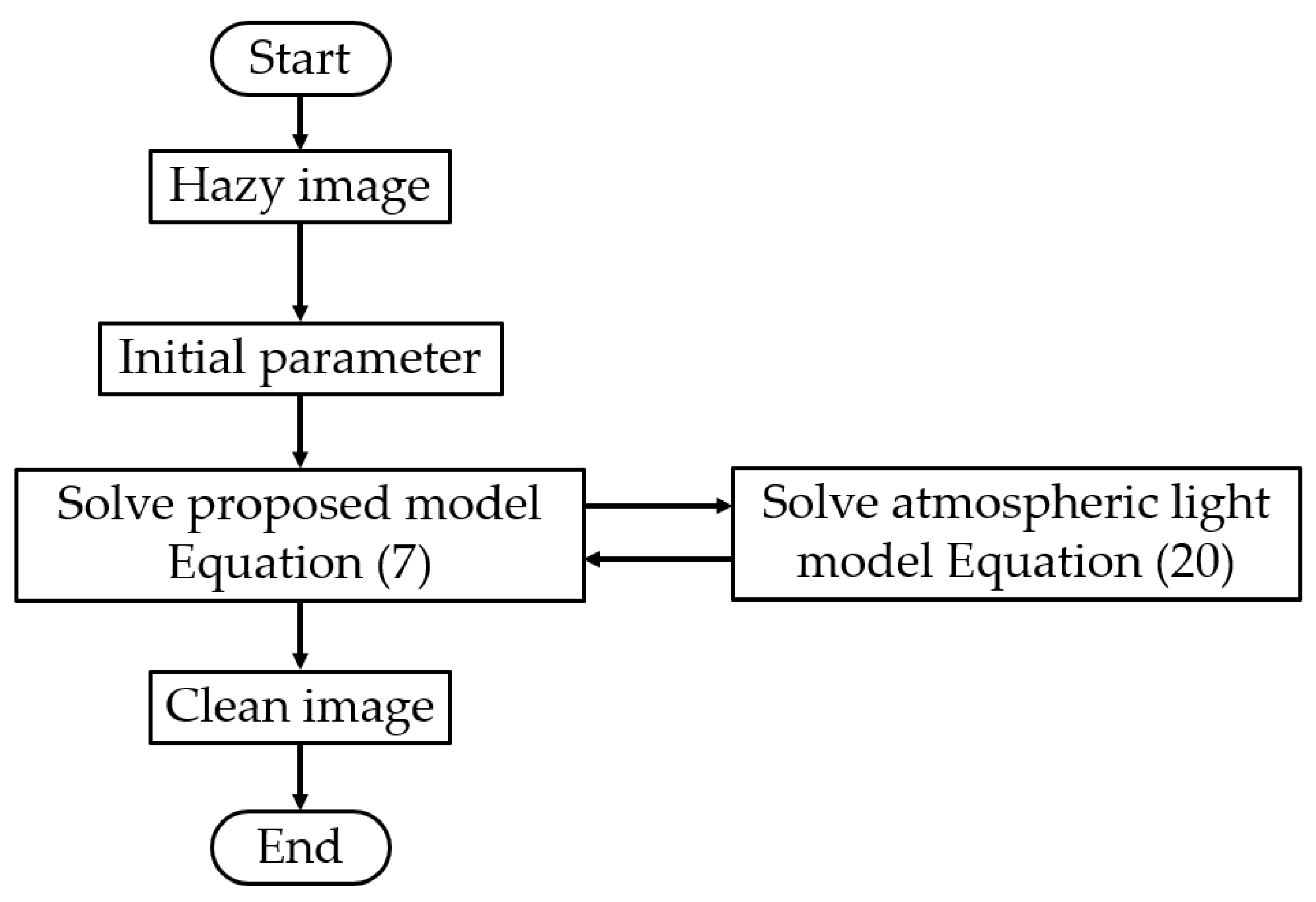
2.6. The Steps of the Proposed Method

The proposed method is an end-to-end (single stage) model, with the following steps:
  • Input: hazy image.
  • Output: clean image.
  • Step 1: Estimate the rough transmission map and the initial atmospheric light. Establish the nitial parameters, and set k1=1 and k2=1;
  • Step 2: Solve Equations (16) and (17), the trained network, and Equation (18);
  • Step 3: Solve Equation (19) and Equations (26)–(28);
  • Step 4: Repeat Step 3, until the iteration exit condition of the atmospheric light estimation is satisfied;
  • Step 5: Repeat Steps 2, 3 and 4, until the iteration exit condition of the transmission map is satisfied;
  • Step 6: Output the transmission map and clean the image.
It is worth noting that the iteration exit condition of the transmission map is k 1 = 50 or | t k 1 1 t k 1 | / ( M N ) 0.004 , where M and N are the image sizes. The iteration exit condition of the atmospheric light estimation is k 2 = 5 . The flow chart of the proposed method is shown in Figure 5:

3. Results

This Section discusses several experiments that were carried out to evaluate the performance of the proposed method. Several state-of-the-art single image dehazing techniques were selected for the comparison, including DCP [2], HLP [3], CAP [4], OTM [52], FFA [53], RefineDNet [54], and CLAHE. The DCP, HLP, Cap, OTM, and MoF were the imaging model-based methods; the FFA and RefineDNet were the deep learning-based methods; and the CLAHE was the image enhancement-based method. The test datasets included synthetic hazy images and real-world images, which were applied to evaluate the dehazing results qualitatively and quantitatively.
To evaluate the performance of the proposed method, two aspects were considered: objective measurement and subjective evaluation. For the objective measurement, two evaluation criteria were examined: the Peak Signal to Noise Ratio (PSNR) and the Structural Similarity Index (SSIM). They were the quantitative evaluation methods. The synthetic hazy images, such as O-hazy [55] and I-hazy [56], were applied. For the subjective evaluation, the above methods were evaluated via subjective judgments about color, haze residual, and noise amplification. Due to the ground truth that real-world images were not available, the no-reference image quality assessment methods were applied, such as information entropy (IE), variance (σ), Blind/Referenceless Image Spatial Quality Evaluator (BRISQUE) [57], and NBIQA, which was introduced in [58].
In the above metrics, the higher the PSNR and SSIM score was, the higher the degree of image restoration was. The high score of IE meant that the dehazing results contained more information. The high score of σ may have indicated that the contrast of the restored image was satisfactory. If the visual effect of the restored image was excellent, it may have implied that the BRISQUE and NBIQA were low.
The tested methods and the evaluation criteria are introduced above. The remainder of this Section is structured as follows: In Section 3.1, the different estimation methods of rough transmission map and initial atmospheric light were tested. In Section 3.2, the dehazing effect via synthesis images was assessed quantitatively. The tested methods were evaluated via real-world images in Section 3.3. Section 3.4 shows the running time of the above dehazing methods.

3.1. Evaluation of Initial Atmospheric Light

In Step 1 of the proposed method, the estimation methods of the rough transmission map and the initial atmospheric light may be important, because the imaging model-based methods are multi-stage. In this Section, the estimation method of the rough transmission map and the initial atmospheric light from DCP, CAP, and HLP techniques were applied to Step 1. The tested image is the synthetic image. Table 1 shows the result.
In Table 1, the results of the three methods are approximate. In the I-hazy dataset, the HLP had the highest score of PSNR, but the DCP had the best SSIM. In the O-hazy dataset, the best score of PSNR was the DCP’s, but the highest SSIM was the CAP’s. In this paper, the DCP was applied to estimate the rough transmission map and the initial atmospheric light because it had two of the highest scores of the quantitative indices.

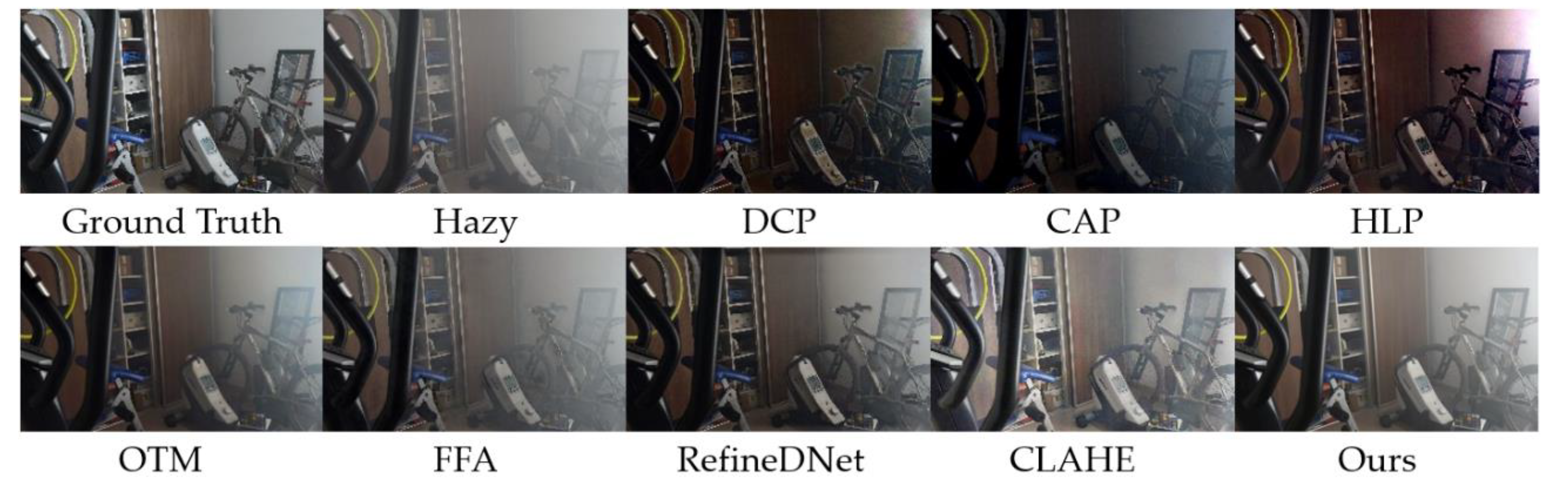
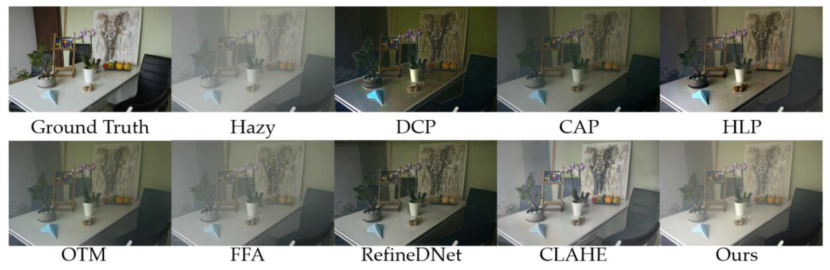
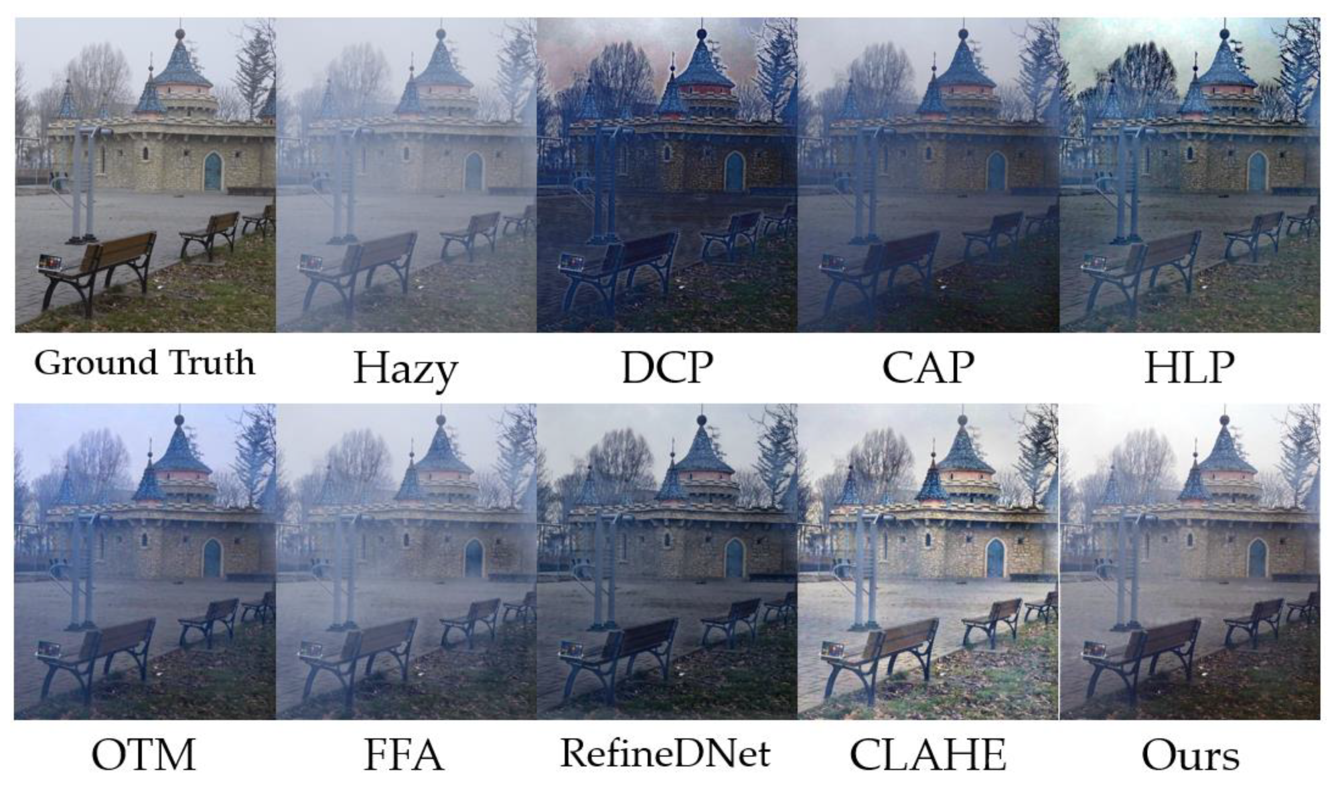
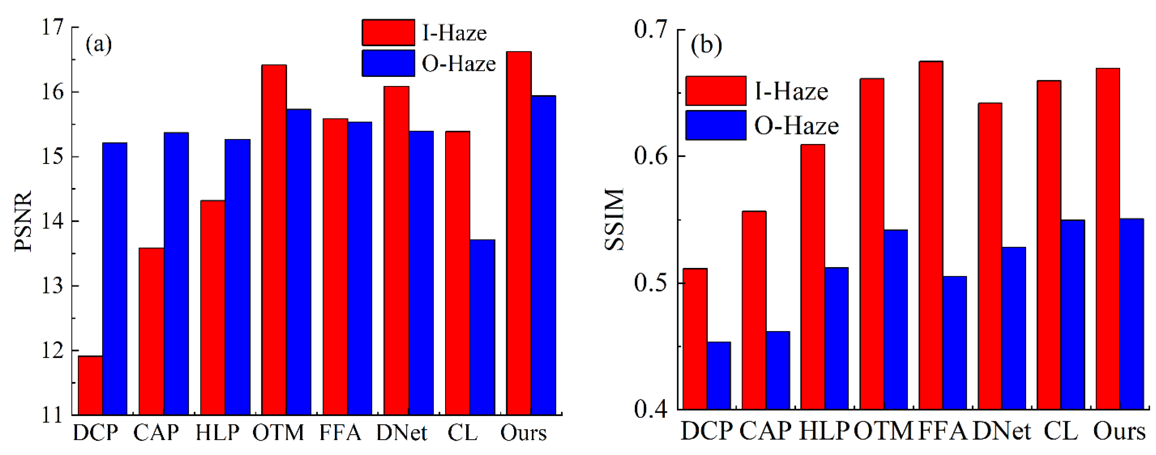
3.2. Evaluation on Synthetic Images

In this Section, the performance of the proposed methods was verified via qualitative image quality evaluation on the synthetic datasets, I-hazy and O-hazy. In I-hazy, there were 30 indoor hazy images and their ground truth. Figure 6 and Figure 7 exhibit the dehazing effect for the above test methods on indoor images, where the ground truth of Figure 6 is nonuniform illumination. Figure 8 and Figure 9 display the hazy removal result on outdoor images, where the background of Figure 8 has a similar color to the haze and contains a sky region (the infinite depth of field), and the background color in Figure 9 differs from the haze color.
For indoor images, all image dehazing methods have a better effect in uniform illumination. In Figure 6 and Figure 7, the result of the imaging model-based methods, such as the DCP, the CAP, and the HLP, lack brightness and contrast, but the proposed method has satisfactory contrast. These results demonstrated that the local and non-local data-driven regularization term could obtain a high-contrast feature for image dehazing. The dehazing results of the FFA had haze residual, but the proposed method alleviated this defect of the FFA, which proved that the imaging model could help the deep learning-based method to remove haze thoroughly. In uniform illumination (as shown in Figure 6), the result of RefineDNet was low-luminance in nonuniform illumination, with defects such as haze residual. Compared with RefineDNet, the results of the proposed method were more stable for nonuniform and uniform illumination. These results indicated that the imaging model combined with deep learning can be applied to different scenarios. It is worth noting that the dehazing effect of the CLAHE and the proposed method is similar. In the proposed model Equation (7) and in Figure 6 and Figure 7, the CLAHE was applied in the data fidelity term, which meant that the dehazing result of the proposed method may be similar to that of the CLAHE in the synthetic indoor hazy image or thin haze.
For outdoor images, the state-of-the-art methods have disappointing dehazing effects. In Figure 8 and Figure 9, the results of the DCP obviously had a halo. In the CAP, the hazy residual seemed to be more significant. The HLP had a poor restoration effect in the sky region, as shown in Figure 8. The OTM displayed such drawbacks as color degradation and haze increase. Compared with the above imaging model-based methods, the results of proposed indicated that the combination of specific physical significance (the imaging model) and abstract nonlinear image features (data-driven regularization term) could improve the dehazing quality more effectively. The FFA does not overcome the phenomenon of haze residual. The dehazing results of RefineDNet lack brightness and blur the edges and textures in the infinite depth of field. Compared with the above deep learning-based method, the proposed local and non-local data-driven regularization term could estimate the image feature purposefully. As shown in Figure 8, the CLAHE can create color distortion, and the defect of haze residual appears in Figure 9 for the CLAHE. These results illustrated that fractional variation can prevent the disadvantages of over-enhancement and color distortion. The proposed method produced results almost as bright as the ground truth images and further reduced the color distortion and halo artifacts. Figure 10a,b illustrates the PSNR and the SSIM of the above dehazing methods, respectively.
In Figure 10, the “DNet” is the RefineDNet, and the “CL” is the CLAHE. Impressively, the proposed methods achieved the highest scores of the PSNR and the SSIM. Regarding the PSNR, the proposed method was superior to other methods in terms of restoration of pixel intensity. Meanwhile, the SSIM of the FFA and the proposed method was similar to that of the I-Haze, and the scores of the OTM, the CLAHE, and the proposed method were similar to those of the O-Haze. Therefore, the proposed method is a satisfactory tool to estimate clean images from a hazy scene.

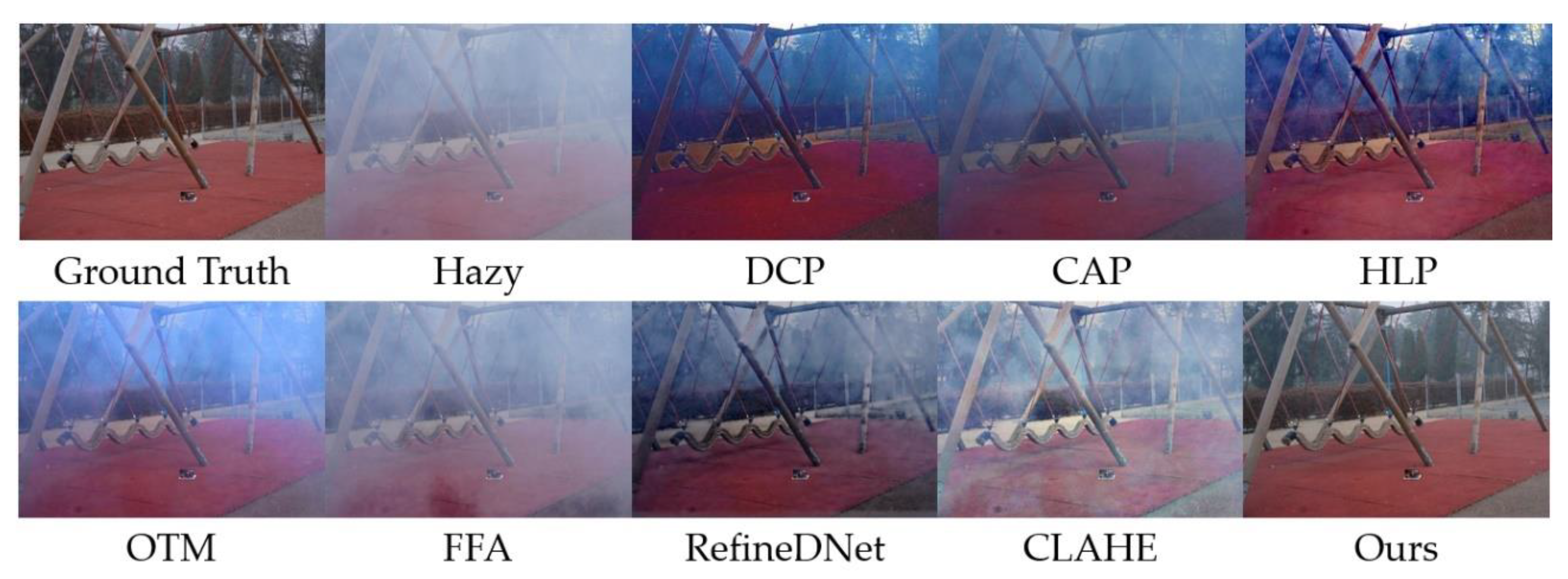
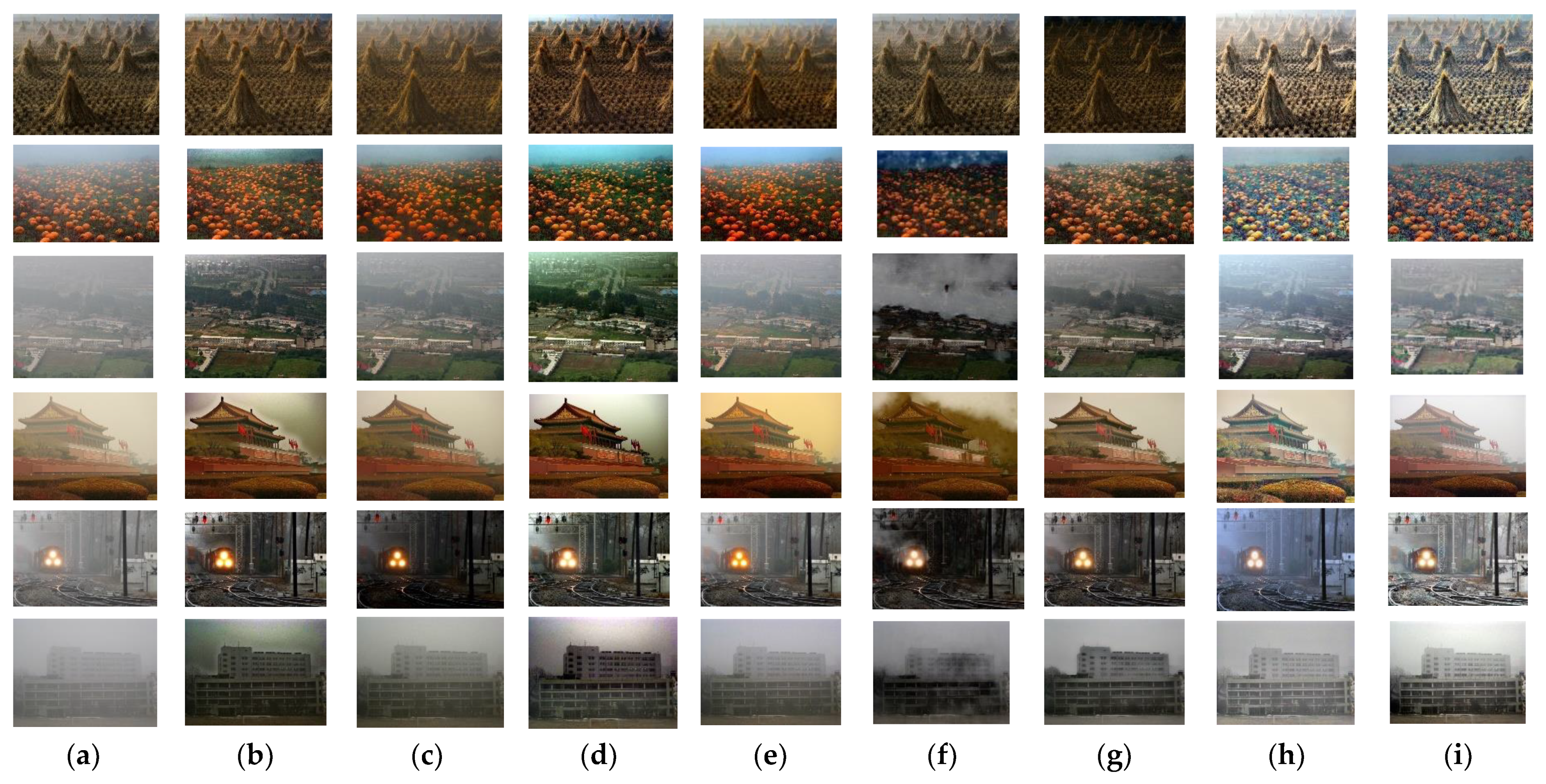
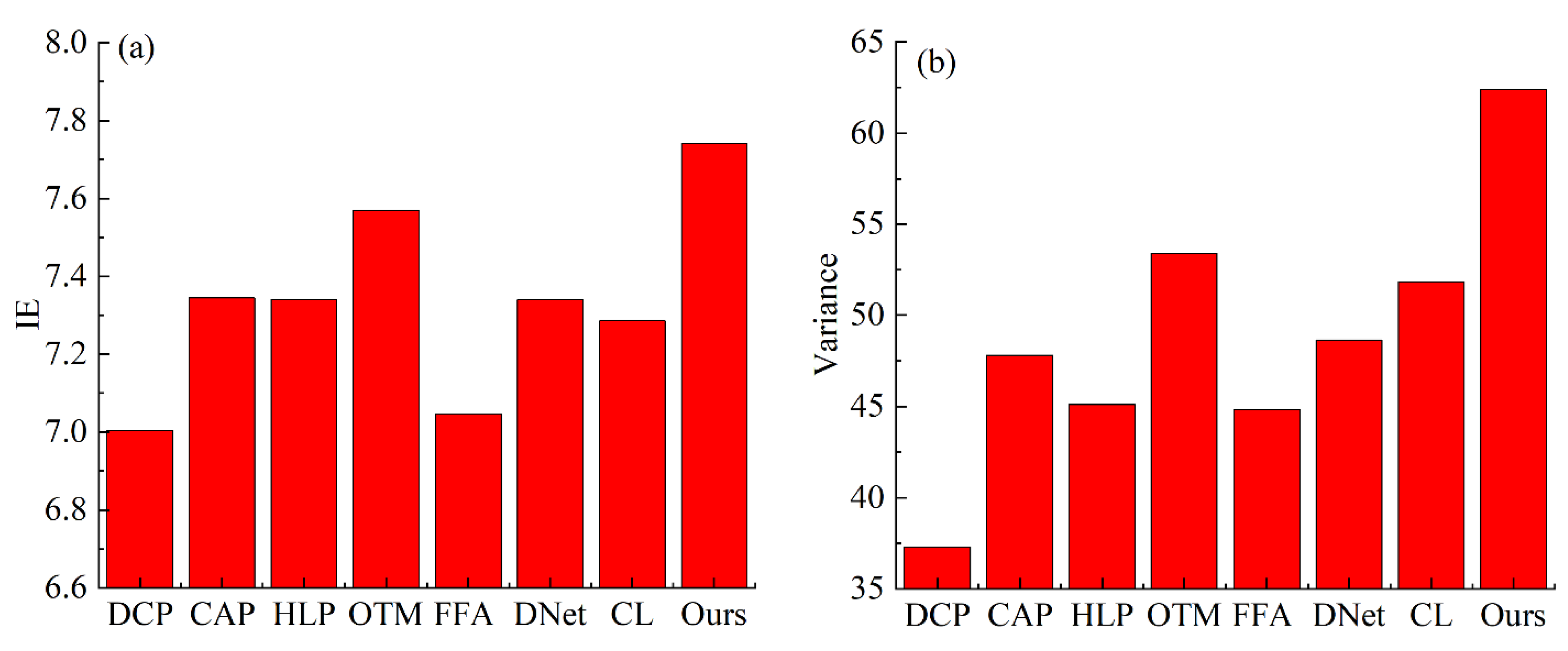
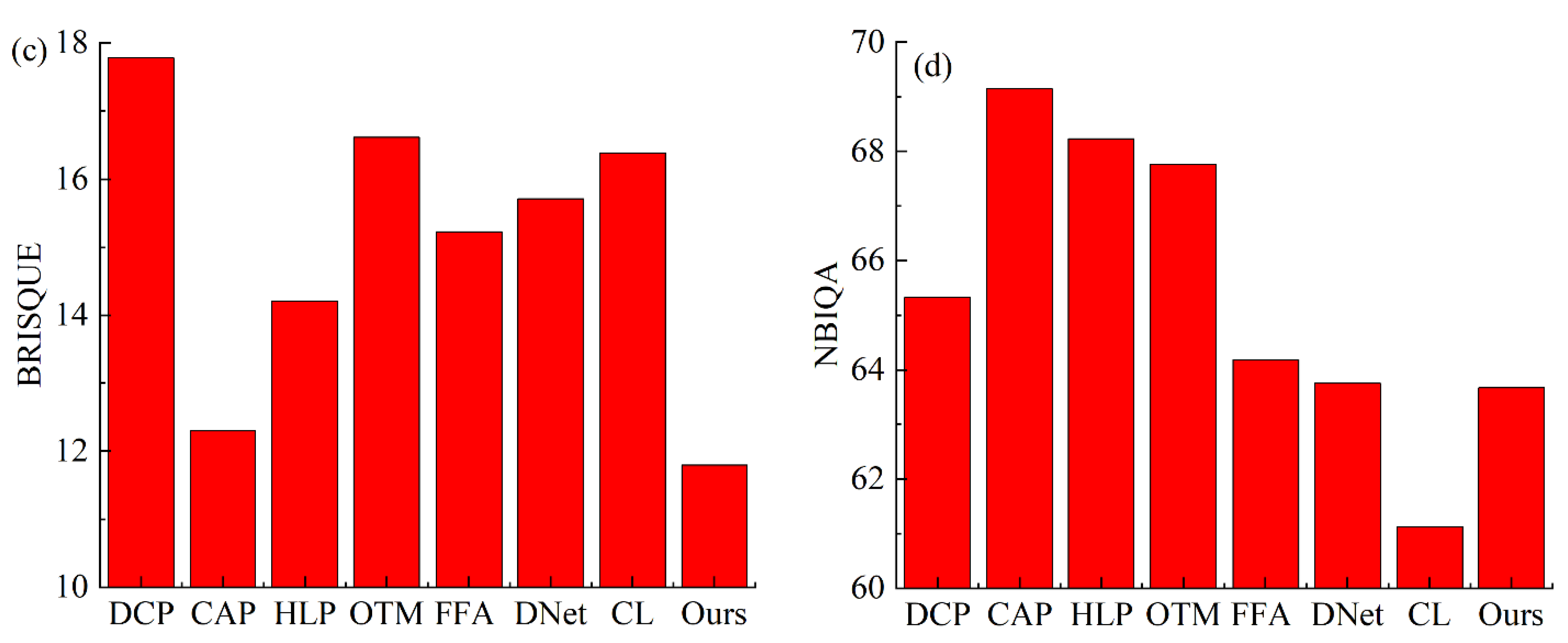
3.3. Evaluation on Real-World Images

Further, the superiority of the proposed method was verified via real-world images. The dehazing effects of several real-world images are illustrated as Figure 11.
Restored via the tested dehazing methods, the majority of the scenes and textures in the above images became obviously clearer. However, the DCP can produce an artificial halo. In the infinity depth of field, the DCP and the HLP produced a miscalculation, and this led the sky to have unusually bright areas. The results of the CAP seemed too dark and some of them had more disappearing edges and textures. The hazy residual was observed from the dehazing image of the OTM. Compared with the above imaging-based methods, the contrast of the proposed method was impressive. Due to the non-local data-driven regularization term, the proposed method could exact the global feature of the image effectively. Fractional variation also seemed to work in regions of the infinite depth of field, which removed the “aureole” in the sky.
The FFA produced some thick haze in the tested image while removing the haze. The phenomenon of brightness degradation was present in the dehazing images of RefineDNet. Unlike the deep learning-based methods, the proposed method was able to estimate high-quality dehazing images. Because the proposed method is based on the haze imaging model, the problem of haze increase (the FFA) was impossible for the proposed method. The local and non-local data-driven regularization item could learn the local and non-local features of the image more purposefully. Hence, the restored results of the proposed method were more robust than those of RefineDNet; the dehazing results “stack”, “train”, and “mansion” of RefineDNet were low-contrast and the dehazing results “flower” and “city” had a vestigial haze, but the proposed method was able to estimate high-quality image.
Because the CLAHE is based on image enhancement, the contrast of the CLAHE is satisfactory visually. However, the results of the CLAHE seemed to suffer from the defects of over-enhancement and hazy residual. However, these defects could be alleviated via fractional variation. In addition, the local data-driven regularization term may further prevent over-enhancement. Therefore, the proposed method had more realistic color effects and fewer artifacts, while enhancing the clearness and removing the haze. In addition, for quantitative analysis, Figure 12 illustrates the IE, σ, BRISQUE, and NBIQA of the above dehazing methods, respectively.
As shown in Figure 12a, the results of the DCP and the FFA had low IE, which could also be proved by the real-world image dehazing experiment, because the artificial halo of the DCP and the produced thick haze via the FFA reduced the edges and textures, drastically. The proposed method obtained the highest IE, which indicated that the proposed method can restore clean edges and textures effectively. The score of σ is shown in Figure 12b, and the proposed method also achieved the best score. These results showed that the contrast of the proposed method is remarkable, which indicates that the objects and textures of the proposed method are sharper than they are for other methods. According to Figure 12c, the proposed method score of BRISQUE is the lowest, which indicates that the restored image has a nice visual effect. However, the best NBIQA was obtained via the CLAHE, and the proposed method was relatively low compared to other methods.

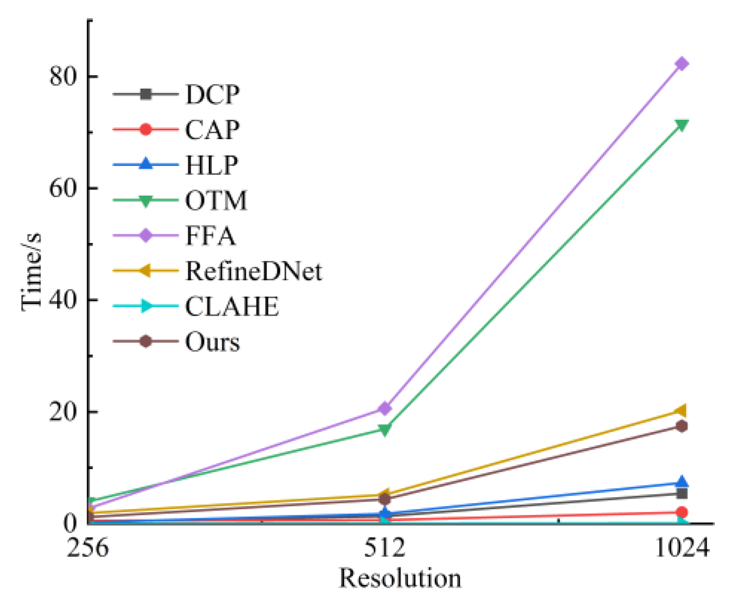
3.4. Running Time Analyze

Running time is another important measure to analyze the performance of the proposed method. In addition to algorithm complexity, the device also played a key role in affecting the running time. With respect to universality, the tested methods were run on different computers with different resolutions. The machines included i5-10300H CPU 8G RAM with GPU NVIDIA GeForce GTX 1650 (Lenovo, Beijing, China). The tested images were from O-hazy, and they were reshaped as 256 × 256, 512 × 512, and 1024 × 1024. Figure 13 shows the running time of the above methods.
As shown in Figure 13, the deep learning-based methods, such as the FFA, RefineDNet, and the proposed method, take longer than other methods. The CLAHE is the fastest method shown in Figure 13. The estimations of the rough transmission map and the initial atmospheric light via the proposed method were slower than those of the imaging model-based methods. However, the running time of the proposed method was the lowest among the deep learning-based methods.

4. Conclusions

In this paper, an image dehazing method based on fractional derivatives and deep learning was proposed. Unlike the traditional deep learning methods, we proposed a novel dehazing model based on a haze imaging formula. The CLAHE was applied as the data field term, which improved the contrast of the proposed method. The fractional derivative was used to smooth the proposed model, avoiding the phenomenon of noise amplification by atmospheric light or the CLAHE. For efficient dehazing, the deep learning method was applied to estimate the local and non-local image features, where the simple CNN was used to obtain the local feature, and the Swin Transformer was applied to estimate non-local features. In addition, the atmospheric light was estimated via an atmospheric veil, and this process was integrated into the iterative solution of the fog model. In the experiment, the proposed method was extensively tested on both synthetic and real-world image datasets, and compared with a variety of different types of single-image dehazing methods, such as the methods based on the imaging model, deep learning, and image enhancement. The qualitative results demonstrated that the proposed method reduces color distortion and brightness degeneration and produces clean edges and textures. Similarly, according to image quality assessments, such as the PSNR, the SSIM, the IE, σ, BRISQUE, and NBIQA, the proposed method was able to improve the dehazing effect significantly.
There are still three main problems restricting the application of the proposed method. First, the running time limits the application of the proposed method in video dehazing with a high frame rate or low-level equipment. Then, studying the adaptive selection method of the parameters, such as the penalty parameter or the number of iterations, is vital. In our previous work [13], we designed a parameter selection method based on convex optimization. However, this method can increase the running time significantly. Hence, on the premise of ensuring the running time, adaptive parameter selection is necessary. Finally, the proposed network architecture can be trained via a semi-supervised or self-supervised framework, which can reduce the dependence of the proposed method on training data and prevent the impact of the synthetic hazy image.
In conclusion, the proposed method can estimate high-quality images from hazy images, and it can be improved in several different ways, including reducing running time, parameter selection, and a training framework.

Author Contributions

Conceptualization, Q.J. and M.L.; formal analysis, Q.J. and B.N.; funding acquisition, Q.J. and M.L.; investigation, B.N. and L.K.; methodology, L.D.; project administration, M.L. and M.H.; resources, F.Z. and L.K.; Software, F.Z.; Supervision, B.N., L.D. and Y.Z.; validation, Y.Z.; visualization, F.Z., L.D., M.H. and Y.Z.; writing—original draft, Q.J.; writing—review & editing, Q.J. and L.K. All authors have read and agreed to the published version of the manuscript.

Funding

This research was funded by the National Key Research and Pevelopment project of China (No. 2018YFF0300804); by the Graduate Innovation Research Project of the Yangtze Delta Region Academy of the Beijing Institute of Technology, Jiaxing (No. GIIP2021-007, No. GIIP2021-006, No. GIIP2021-011, No. GIIP2021-012); and by the National Natural Science Foundation of China (No. 11774031).

Institutional Review Board Statement

Not applicable.

Informed Consent Statement

Not applicable.

Data Availability Statement

The tested image is available at [45,46], and the code can be obtained from the first-named author.

Conflicts of Interest

The authors declare no conflict of interest.

Appendix A

Due to the number of parameters and equations in this paper, this Appendix elaborates on each parameter.
Table A1. Detailed annotation of parameters and symbols.
No.SymbolAnnotationType
1AAtmospheric lightVector
2 C ( · ) Local regularization termFunction
3 D x α Horizontal direction right fractional operatorOperator
4 ( D x α ) * Horizontal direction left fractional operatorOperator
5 ( D x α ) * D x α Horizontal direction composite fractional operatorOperator
6 D y α Vertical direction right fractional operatorOperator
7 ( D y α ) * Vertical direction right fractional operatorOperator
8 ( D y α ) * D y α Vertical direction composite fractional operatorOperator
9 d k Size of key in MSANumber
10 E ( · ) The proposed networkFunction
11EUnit matrixMatrix
12IHazy imageMatrix
13 I C L A H E Optimized hazy image via CLAHEMatrix
14IPixel coordinatesNumber
15JIdeal imageMatrix
16 J ^ Ideal image, variableMatrix
17JPixel coordinatesNumber
18KKey of MSAMatrix
19KGird size of standard discretization techniqueNumber
20 k 1 Iterations number of transmission map estimationNumber
21 k 2 Iterations number of atmospheric light estimationNumber
22LNumber of train dataNumber
23MSize of imageNumber
24MNumber of grids of standard discretization techniqueNumber
25NSize of imageNumber
26QQuery of MSAMatrix
27 s g n ( · ) Symbolic functionFunction
28TTransmission mapMatrix
29 t ^ Transmission map, variableMatrix
30 T ( · ) Non-local regularization termFunction
31VValue of MSA only in Equation (14)Matrix
32VAtmospheric veilMatrix
33VAuxiliary variableMatrix
34WAuxiliary variableMatrix
35XAuxiliary variableMatrix
36 α orderNumber
37 λ 1 ,   λ 2 ,   λ 3 ,   λ 4 ,   λ 5 Regularization parameterNumber
38 η 1 ,   η 2 ,   η 3 Penalty parameterNumber
39ΘThe proposed network parametersMatrix
40 θ Balance parameter in Equation (15)Number
41 | · | 1 ,   | · | 2 1-norm, 2-normFunction

References

  1. Galdran, A.; Javier, V.C.; David, P.; Marcelo, B. Enhanced Variational Image Dehazing. SIAM J. Imaging Sci. 2015, 8, 1519–1546. [Google Scholar] [CrossRef] [Green Version]
  2. He, K.; Sun, J.; Tang, X. Single Image Haze Removal Using Dark Channel Prior. IEEE Trans. Pattern Anal. Mach. Intell. 2010, 33, 2341–2353. [Google Scholar] [CrossRef] [PubMed]
  3. Berman, D.; Treibitz, T.; Avidan, S. Single Image Dehazing Using Haze-Lines. IEEE Trans. Pattern Anal. Mach. Intell. 2018, 42, 720–734. [Google Scholar] [CrossRef] [PubMed]
  4. Zhu, Q.; Mai, J.; Shao, L. A Fast Single Image Haze Removal Algorithm Using Color Attenuation Prior. IEEE Trans. Image Process. 2015, 24, 3522–3533. [Google Scholar] [CrossRef] [Green Version]
  5. He, K.M.; Sun, J.; Tang, X.O. Guided Image Filtering. IEEE Trans. Pattern Anal. 2013, 35, 1397–1409. [Google Scholar] [CrossRef]
  6. Li, Z.; Zheng, J.; Zhu, Z.; Yao, W.; Wu, S. Weighted Guided Image Filtering. IEEE Trans. Image Process. 2014, 24, 120–129. [Google Scholar] [CrossRef]
  7. Kou, F.; Chen, W.; Wen, C.; Li, Z. Gradient Domain Guided Image Filtering. IEEE Trans. Image Process. 2015, 24, 4528–4539. [Google Scholar] [CrossRef]
  8. Ochotorena, C.N.; Yamashita, Y. Anisotropic Guided Filtering. IEEE Trans. Image Process. 2019, 29, 1397–1412. [Google Scholar] [CrossRef]
  9. Selesnick, I. Generalized Total Variation: Tying the Knots. IEEE Signal Process. Lett. 2015, 22, 2009–2013. [Google Scholar] [CrossRef] [Green Version]
  10. Bredies, K.; Kunisch, K.; Pock, T. Total generalized variation. SIAM J. Imaging Sci. 2010, 3, 492–526. [Google Scholar] [CrossRef]
  11. Gilboa, G.; Sochen, N.; Zeevi, Y.Y. Image enhancement and denoising by complex diffusion processes. IEEE T. Pattern Anal. 2004, 26, 1020–1036. [Google Scholar] [CrossRef] [PubMed]
  12. Liu, Q.; Gao, X.; He, L.; Lu, W. Single Image Dehazing with Depth-Aware Non-Local Total Variation Regularization. IEEE Trans. Image Process. 2018, 27, 5178–5191. [Google Scholar] [CrossRef] [PubMed]
  13. Jiao, Q.; Liu, M.; Li, P.; Dong, L.; Hui, M.; Kong, L.; Zhao, Y. Underwater Image Restoration via Non-Convex Non-Smooth Variation and Thermal Exchange Optimization. J. Mar. Sci. Eng. 2021, 9, 570. [Google Scholar] [CrossRef]
  14. Parisotto, S.; Lellmann, J.; Masnou, S.; Schönlieb, C.-B. Higher-Order Total Directional Variation: Imaging Applications. SIAM J. Imaging Sci. 2020, 13, 2063–2104. [Google Scholar] [CrossRef]
  15. Chan, R.H.; Lanza, A.; Morigi, S.; Sgallari, F. An Adaptive Strategy for the Restoration of Textured Images using Fractional Order Regularization. Numer. Math. Theory Methods Appl. 2013, 6, 276–296. [Google Scholar] [CrossRef]
  16. Bilgi, C.Y.; Mürvet, K. Fractional Differential Equation-Based Instantaneous Frequency Estimation for Signal Reconstruction. Fractal Fract. 2021, 5, 83. [Google Scholar]
  17. Svynchuk, O.; Barabash, O.; Nikodem, J.; Kochan, R.; Laptiev, O. Image Compression Using Fractal Functions. Fractal Fract. 2021, 5, 31. [Google Scholar] [CrossRef]
  18. Zhang, X.; Liu, R.; Ren, J.; Gui, Q. Adaptive Fractional Image Enhancement Algorithm Based on Rough Set and Particle Swarm Optimization. Fractal Fract. 2022, 6, 100. [Google Scholar] [CrossRef]
  19. Xu, K.; Liu, J.; Miao, J.; Liu, F. An improved SIFT algorithm based on adaptive fractional differential. J. Ambient Intell. Humaniz. Comput. 2018, 10, 3297–3305. [Google Scholar] [CrossRef]
  20. Luo, X.; Zeng, T.; Zeng, W.; Huang, J. Comparative analysis on landsat image enhancement using fractional and integral differential operators. Computing 2019, 102, 247–261. [Google Scholar] [CrossRef]
  21. Yuan, H.; Liu, C.; Guo, Z.; Sun, Z. A Region-Wised Medium Transmission Based Image Dehazing Method. IEEE Access 2017, 5, 1735–1742. [Google Scholar] [CrossRef]
  22. Guo, F.; Qiu, J.; Tang, J. Single Image Dehazing Using Adaptive Sky Segmentation. IEEJ Trans. Electr. Electron. Eng. 2021, 16, 1209–1220. [Google Scholar] [CrossRef]
  23. Liu, Y.; Li, H.; Wang, M. Single Image Dehazing via Large Sky Region Segmentation and Multiscale Opening Dark Channel Model. IEEE Access 2017, 5, 8890–8903. [Google Scholar] [CrossRef]
  24. Wang, W.; Yuan, X.; Wu, X.; Liu, Y. Dehazing for images with large sky region. Neurocomputing 2017, 238, 365–376. [Google Scholar] [CrossRef]
  25. LeCun, Y.; Bengio, Y.; Hinton, G. Deep learning. Nature 2015, 521, 436–444. [Google Scholar] [CrossRef] [PubMed]
  26. Zhou, Y.; Chen, Z.H.; Sheng, B.; Li, P.; Kim, J.; Wu, E.H. AFF-Dehazing: Attention-based feature fusion network for low-light image Dehazing. Comput. Animat. Virt. Worlds 2021, 32, e2011. [Google Scholar] [CrossRef]
  27. Sun, Z.; Zhang, Y.; Bao, F.; Shao, K.; Liu, X.; Zhang, C. ICycleGAN: Single image dehazing based on iterative dehazing model and CycleGAN. Comput. Vis. Image Underst. 2020, 203, 103133. [Google Scholar] [CrossRef]
  28. Zhang, S.; He, F. DRCDN: Learning deep residual convolutional dehazing networks. Vis. Comput. 2019, 36, 1797–1808. [Google Scholar] [CrossRef]
  29. Li, B.; Gou, Y.; Gu, S.; Liu, J.Z.; Zhou, J.T.; Peng, X. You Only Look Yourself: Unsupervised and Untrained Single Image Dehazing Neural Network. Int. J. Comput. Vis. 2021, 129, 1754–1767. [Google Scholar] [CrossRef]
  30. Golts, A.; Freedman, D.; Elad, M. Unsupervised Single Image Dehazing Using Dark Channel Prior Loss. IEEE Trans. Image Process. 2020, 29, 2692–2701. [Google Scholar] [CrossRef] [Green Version]
  31. Kumar, A.; Ahmad, M.O.; Swamy, M.N.S. Image Denoising Based on Fractional Gradient Vector Flow and Overlapping Group Sparsity as Priors. IEEE Trans. Image Process. 2021, 30, 7527–7540. [Google Scholar] [CrossRef] [PubMed]
  32. Li, C.; Zeng, F. Numerical Methods for Fractional Calculus, 3rd ed.; CRC Press: Abingdon, UK, 2015; pp. 97–124. [Google Scholar]
  33. Diethelm, K. An Algorithm for The Numerical Solution of Differential Equations of Fractional Order. Electron. Trans. Numer. Anal. 1997, 5, 1–6. [Google Scholar]
  34. Huang, L.D.; Zhao, W.; Wang, J.; Sun, Z.B. Combination of contrast limited adaptive histogram equalisation and discrete wavelet transform for image enhancement. IET Image Process. 2015, 9, 908–915. [Google Scholar]
  35. Cui, T.; Tian, J.D.; Wang, E.D.; Tang, Y.D. Single image dehazing by latent region- segmentation based transmission estimation and weighted L 1 -norm regularization. IET Image Process. 2017, 11, 145–154. [Google Scholar] [CrossRef] [Green Version]
  36. Aubert, G.; Vese, L. A Variational Method in Image Recovery. SIAM J. Numer. Anal. 1997, 34, 1948–1979. [Google Scholar] [CrossRef]
  37. Cheng, K.; Du, J.; Zhou, H.; Zhao, D.; Qin, H. Image super-resolution based on half quadratic splitting. Infrared Phys. Technol. 2020, 105, 103193. [Google Scholar] [CrossRef]
  38. Zhang, S.; He, F.; Ren, W. NLDN: Non-local dehazing network for dense haze removal. Neurocomputing 2020, 410, 363–373. [Google Scholar] [CrossRef]
  39. Dekel, T.; Michaeli, T.; Irani, M.; Freeman, W.-T. Revealing and Modifying Non-Local Variations in a Single Image. ACM T. Graph. 2015, 34, 227. [Google Scholar] [CrossRef] [Green Version]
  40. Hu, H.-M.; Zhang, H.; Zhao, Z.; Li, B.; Zheng, J. Adaptive Single Image Dehazing Using Joint Local-Global Illumination Adjustment. IEEE Trans. Multimed. 2019, 22, 1485–1495. [Google Scholar] [CrossRef]
  41. Karen, S.; Andrew, Z. Two-Stream Convolutional Networks for Action Recognition in Videos. arXiv 2014, arXiv:1406.2199. [Google Scholar]
  42. Liu, Z.; Lin, Y.; Cao, Y.; Hu, H.; Wei, Y.; Zhang, Z.; Lin, S.; Guo, B. Swin Transformer: Hierarchical Vision Transformer using Shifted Windows. arXiv 2021, arXiv:2103.14030. [Google Scholar]
  43. He, K.; Zhang, X.; Ren, S.; Sun, J. Deep residual learning for image recognition. In Proceedings of the 2016 IEEE Conference on Computer Vision and Pattern Recognition (CVPR), Las Vegas, NV, USA, 27–30 June 2016; pp. 770–778. [Google Scholar] [CrossRef] [Green Version]
  44. Zhang, X.; Sun, G.; Jia, X.; Wu, L.; Zhang, A.; Ren, J.; Fu, H.; Yao, Y. Spectral–Spatial Self-Attention Networks for Hyperspectral Image Classification. IEEE Trans. Geosci. Remote Sens. 2021, 60, 1–15. [Google Scholar] [CrossRef]
  45. Dosovitskiy, A.; Beyer, L.; Kolesnikov, A.; Weissenborn, D.; Zhai, X.H.; Unterthiner, T.; Dehghani, M.; Minderer, M.; Heigold, G.; Gelly, S.; et al. An Image is Worth 16 × 16 Words: Transformers for Image Recognition at Scale. arXiv 2020, arXiv:2010.11929. [Google Scholar]
  46. Fan, H.; Xiong, B.; Mangalam, K.; Li, Y.; Yan, Z.; Malik, J.; Feichtenhofer, C. Multiscale Vision Transformers. arXiv 2021, arXiv:2104.11227. [Google Scholar]
  47. Lin, T.-Y.; Maire, M.; Belongie, B.; Bourdev, L.; Girshick, R.; Hays, J.; Perona, P.; Ramanan, D.; Zitnick, C.-L.; Dollár, P. Microsoft COCO: Common Objects in Context. arXiv 2015, arXiv:1405.0312. [Google Scholar]
  48. Chambolle, A.; Pock, T. A First-Order Primal-Dual Algorithm for Convex Problems with Applications to Imaging. J. Math. Imaging Vis. 2010, 40, 120–145. [Google Scholar] [CrossRef] [Green Version]
  49. He, N.; Wang, J.-B.; Zhang, L.-L.; Lu, K. Convex optimization based low-rank matrix decomposition for image restoration. Neurocomputing 2016, 172, 253–261. [Google Scholar] [CrossRef]
  50. Yu, K.; Cheng, Y.; Li, L.; Zhang, K.; Liu, Y.; Liu, Y. Underwater Image Restoration via DCP and Yin–Yang Pair Optimization. J. Mar. Sci. Eng. 2022, 10, 360. [Google Scholar] [CrossRef]
  51. Tare, J.P.; Hautière, N. Fast visibility restoration from a single color or gray level image. In Proceedings of the IEEE 12th International Conference on Computer Vision, Kyoto, Japan, 29 September–2 October 2009. [Google Scholar]
  52. Ngo, D.; Seungmin, L.; Kang, B.S. Robust Single-Image Haze Removal Using Optimal Transmission Map and Adaptive At-mospheric Light. Robust Single-Image Haze Removal Using Optimal Transmission Map and Adaptive Atmospheric Light. Remote Sens. 2020, 12, 2233. [Google Scholar] [CrossRef]
  53. Qin, X.; Wang, Z.; Bai, Y.; Xie, X.; Jia, H. FFA-Net: Feature Fusion Attention Network for Single Image Dehazing. In Proceedings of the AAAI Conference on Artificial Intelligence, Honolulu, HI, USA, 17–19 January 2019. [Google Scholar]
  54. Zhao, S.; Zhang, L.; Shen, Y.; Zhou, Y. RefineDNet: A Weakly Supervised Refinement Framework for Single Image Dehazing. IEEE Trans. Image Process. 2021, 30, 3391–3404. [Google Scholar] [CrossRef]
  55. Ancuti, C.O.; Ancuti, C.; Timofte, R.; Christophe, D.V. O-HAZE: A dehazing benchmark with real hazy and haze-free outdoor images. In Proceedings of the IEEE Conference on Computer Vision and Pattern Recognition, Salt Lake City, UT, USA, 18–22 June 2018. [Google Scholar]
  56. Ancuti, C.O.; Ancuti, C.; Timofte, R.; Christophe, D.V. I-HAZE: A dehazing benchmark with real hazy and haze-free indoor images. In Proceedings of the Advanced Concepts for Intelligent Vision Systems, Poitiers, France, 24–27 September 2018. [Google Scholar]
  57. Mittal, A.; Moorthy, A.K.; Bovik, A. No-Reference Image Quality Assessment in the Spatial Domain. IEEE Trans. Image Process. 2012, 21, 4695–4708. [Google Scholar] [CrossRef] [PubMed]
  58. Ou, F.-Z.; Wang, Y.-G.; Zhu, G. A Novel Blind Image Quality Assessment Method Based on Refined Natural Scene Statistics. In Proceedings of the IEEE International Conference on Image Processing, Taipei, Taiwan, 22–25 December 2019. [Google Scholar]
Figure 1. The architecture of the proposed two-streams network. To solve Equation (12), the first term of Equation (12) was designed as the upper stream, the second term was designed as the lower stream, and the third term could be calculated directly.
Fractalfract 06 00262 g001
Figure 2. An illustration of CNN.
Fractalfract 06 00262 g002
Figure 3. The architecture of the two successive Swin Transformer blocks. W-MSA and SW-MSA are multi-head self-attention modules with regular and shifted windowing configurations, respectively.
Fractalfract 06 00262 g003
Figure 4. The architecture of the self-attention block.
Fractalfract 06 00262 g004
Figure 5. An illustration of the proposed method.
Fractalfract 06 00262 g005
Figure 6. The dehazing effect of an indoor image with nonuniform illumination. The first row, from left to right, shows the ground truth, the synthetic hazy image, and the dehazing of the DCP, the CAP, and the HLP. The second row, from left to right, shows the dehazing methods of the OTM, the FFA, RefineDNet, and the CLAHE, as well as ours (the authors’).
Fractalfract 06 00262 g006
Figure 7. The dehazing effect of an indoor image with uniform illumination. The first row, from left to right, shows the ground truth, the synthetic hazy image, and the dehazing of the DCP, the CAP, and the HLP. The second row, from left to right, shows the dehazing methods of the OTM, the FFA, RefineDNet, and the CLAHE, as well as ours (the authors’).
Fractalfract 06 00262 g007
Figure 8. The dehazing effect of an outdoor image with a sky region. The first row, from left to right, shows the ground truth, the synthetic hazy image, and the dehazing of the DCP, the CAP, and the HLP. The second row, from left to right, shows the dehazing of the OTM, the FFA, RefineDNet, and the CLAHE, as well as ours (the authors’).
Fractalfract 06 00262 g008
Figure 9. The dehazing effect of an outdoor image without a sky region. The first row, from left to right, shows the ground truth, the synthetic hazy image, and the dehazing of the DCP, the CAP, and the HLP. The second row, from left to right, shows the dehazing of the OTM, the FFA, RefineDNet, and the CLAHE, as well as ours (the authors’).
Fractalfract 06 00262 g009
Figure 10. The PSNR and the SSIM of synthetic hazy images. (a) The PSNR of tested methods with different datasets. (b) The SSIM of tested methods with different datasets.
Fractalfract 06 00262 g010
Figure 11. The dehazing results of real-world hazy images. From top to bottom are “stack”, “flower”, “city”, “Tiananmen”, “train”, and “mansion”. (a) The origin hazy images. (b) The dehazing result of the DCP. (c) The dehazing effect of the CAP. (d) The dehazing effect of the HLP. (e) The dehazing effect of the OTM. (f) The dehazing effect of the FFA. (g) The dehazing effect of RefineDNet. (h) The dehazing effect of the CLAHE. (i) The dehazing effect of the authors’ proposed method.
Fractalfract 06 00262 g011
Figure 12. The dehazing results of the real-world hazy image. (a) The average score of IE for the dehazing result. (b) The average score of variances for the dehazing result. (c) The average score of BRISQUE for the dehazing result. (d) The average score of NBIQA for the dehazing result.
Fractalfract 06 00262 g012aFractalfract 06 00262 g012b
Figure 13. The computation time in seconds of compared approaches to dehazing methods.
Fractalfract 06 00262 g013
Table 1. Comparison of three rough transmission map and initial atmospheric light estimation methods.
MethodI-HazyO-Hazy
PSNRSSIMPSNRSSIM
DCP16.420.6715.940.55
CAP16.370.6615.870.58
HLP16.480.6415.890.56
Publisher’s Note: MDPI stays neutral with regard to jurisdictional claims in published maps and institutional affiliations.

