Article

A New Adaptive Robust Sliding Mode Control Approach for Nonlinear Singular Fractional-Order Systems

1
College of Sciences, Northeastern University, Shenyang 110819, China
2
State Key Laboratory of Synthetical Automation for Process Industries, Northeastern University, Shenyang 110819, China
*
Authors to whom correspondence should be addressed.
Fractal Fract. 2022, 6(5), 253; https://doi.org/10.3390/fractalfract6050253
Submission received: 25 March 2022 / Revised: 24 April 2022 / Accepted: 3 May 2022 / Published: 6 May 2022

Abstract

:
This article focuses on designing an adaptive sliding mode controller via state and output feedback for nonlinear singular fractional-order systems (SFOSs) with mismatched uncertainties. Firstly, on the basis of extending the dimension of the SFOS, a new integral sliding mode surface is constructed. Through this special sliding surface, the sliding mode of the descriptor system does not contain a singular matrix E. Then, the sufficient conditions that ensure the stability of sliding mode motion are given by using linear matrix inequality. Finally, the control law based on an adaptive mechanism that is used to update the nonlinear terms is designed to ensure the SFOS satisfies the reaching condition. The applicability of the proposed method is illustrated by a practical example of a fractional-order circuit system and two numerical examples.

1. Introduction

Fractional order systems (FOSs) are especially suitable for describing the memory, heredity, mechanical and electrical properties of various materials, so they are widely used in various practical applications [1,2,3]. By constructing solvable linear matrix inequalities (LMIs), the robust control problems in FOSs can be effectively solved. In [4,5,6], the stabilization problem of FOSs is solved by designing an observer. In [7], an LMI based on criteria to ensure the stability or stabilization of FOSs for a given order α : 0 < α < 2 was provided.
The generalized system model can describe a broader practical system, which is more general than normal systems. Therefore, it is very important to study the generalized system model [8,9,10]. As for SFOSs, a large amount of research for the problems of admissibility and robust stabilization has been reported recently in [11]. In proving the admissibility of SFOSs, the authors in [12,13] solve the problem by transforming the SFOSs into normal FOSs through a specific feedback controller. On the other hand, when the fractional-order 0 < α < 1 , the authors in [14] extend the admissibility method of integer order singular systems to SFOSs and present three different LMI conditions for the admissibility [15]. Correspondingly, in [16], this problem with 1 < α < 2 is considered, whereas Theorem 3 in [16] is a bilinear matrix inequality, which is difficult to be used to solve the output feedback control problem of SFOSs. Since state variables are often difficult to obtain in practical applications, it is meaningful to research the design of the output feedback controller. The authors in [17] provide the LMI condition to solve the output feedback control problem by making the output matrix C satisfy a particular construct. The authors in [18] investigate the robust stabilization problem for T-S fuzzy FOSs via output feedback control, but this approach is difficult apply to SFOSs with 0 < α < 1 . In [19], this defect has been overcome by using an intermediate variable to construct a strict LMI condition. However, this method needs to first know the information of the status variable, which is conservative.
As a mature control strategy, sliding mode control [20,21,22,23] (SMC) has recently received much attention in FOSs [24,25]. In practical applications, uncertain nonlinear systems [26] with disturbances are ubiquitous, and the SMC is a nonlinear robust control method, which can maintain the stability of systems. In [27], a reduced dimension of a sliding surface is constructed to get rid of the influence of nonlinear terms, and the control law is designed to force the FOSs to move along the sliding surface. A discrete-time fractional-order SMC scheme is proposed in [28]. In [29], the authors design a sliding mode controller for fractional-order financial systems. In [30], the integral sliding surface is designed for SFOSs, the attractive part of the this surface is that it enables the trajectory of SFOSs to start from the constructed sliding surface, which makes SFOSs more robust.
Any actual system has varying degrees of uncertainty. For example, the structure and parameters of the mathematical model describing the controlled object are not necessarily known by the designer in advance. In the face of these uncertainties, to design appropriate control function to make a specific performance index reach and maintain the optimum or approximate optimum, adaptive control [31] is proposed. Adaptive control, as a control method to estimate the nonlinear terms that are unknown in FOSs, is presented in [32]. In [33], the adaptive backstepping control schemes are proposed for FOSs. The authors in [34] used a fuzzy adaptive state observer to estimate the unmeasured state. In [35], the problem of adaptive control for uncertain T-S fuzzy FOSs with saturated control inputs is addressed. It is worth noting that adaptive control also plays an important role in the design of a sliding mode controller for FOSs [36,37,38]. The authors in [39] study the adaptive fuzzy SMC problem for chaotic FOSs. In [40], the authors propose the adaptive SMC method for nonlinear FOSs. For mismatched disturbances in nonlinear systems, the authors in [41] provide a novel scheme based on a disturbance observer to estimate the disturbances of FOSs. In [42], the problem of real-time SMC for dynamical systems is solved. Furthermore, the authors in [43] develop an adaptive sliding mode controller for time-varying delay singular systems. Furthermore, adaptive SMC is also of great significance in practical applications. For example, [44,45] studied adaptive SMC of rubber-tired gantry crane. By using adaptive fractional-order SMC, the controller can track the driving state well in the case of parameter uncertainty and unknown disturbance. Since the adaptive sliding mode controller can solve the matching uncertainty with an unknown upper bound and input saturation, it has more far-reaching significance. For example, it can eliminate the condition of the nonlinear term [46]. However, the design of the adaptive sliding mode controller via output feedback for SFOSs [47] with fractional-order 0 < α < 1 is still a difficult and open problem.
Inspired by the aforementioned discussions, the main contributions of this paper are listed below.
  (1) At present, most papers need feedback control for normal SFOSs [11,12,13]. Since the special sliding surface is constructed in this paper, which leads to the sliding motion being a normalized FOS, this approach can be regarded as a new normalization technique without the feedback control.
  (2) On the basis of extending the dimension of the SFOS, a new integral sliding mode surface is constructed. Through this special sliding surface, the sliding mode of the descriptor system does not contain a singular matrix E. Thus, we can use the stability theorem of the normal system to study the stability of the sliding mode. In [8,9], their sliding modes contain a singular matrix E, which can only be studied by the admissibility theorem of the singular system.
  (3) The SMC stabilization problems with state feedback and output feedback are both investigated, and the main results are in terms of LMIs. In addition, the output feedback SMC scheme does not need to calculate the intermediate variable, which is more effective than [19].
  (4) The adaptive SMC law is proposed such that the finite-time reachability of the sliding surface can be guaranteed. Furthermore, it can be deal with the nonlinear terms. The restriction that the norm of the disturbance of the system should be known in [4] is removed.
In the following, Section 2 describes the preliminaries. In Section 3, state and output feedback SMC is considered. In Section 4, the proposed methods are evaluated by a practical example and two numerical examples. Finally, conclusions of this study are provided in Section 5.
Notations: In this paper, M T is the transpose of matrix M . Matrix X > 0 ( < 0 ) means that the X is positive (negative) definite. ∗ indicates the symmetric part of a matrix, such as S N Z = S N N T Z . | | · | | represents the induction norm of a matrix or the Euclidean norm of a vector. a = sin ( α π 2 ) , b = cos ( α π 2 ) and sym ( Y ) = Y + Y T for short in the sequel.

2. Preliminaries

Consider the following nonlinear SFOS with fractional-order 0 < α < 1
E D α x ( t ) = ( A + Δ A ) x ( t ) + B ( u ( t ) + g ( x ( t ) , t ) ) , y ( t ) = C x ( t ) ,
where x ( t ) R n , y ( t ) R p are the system state and the measured output, respectively. u ( t ) R l is the control input. E R n × n is a singular matrix and rank ( E ) = m < n . A R n × n , B R n × l and C R p × n . Δ A R n × n is the mismatched uncertain matrix, assuming that Δ A = U F ( t ) V , where U and V are appropriate dimensions matrices, and F ( t ) is an unknown matrix function which satisfies F T ( t ) F ( t ) I . Moreover, the nonlinear unknown function g ( x ( t ) , t ) represents the matched uncertainty or disturbance, which is assumed to satisfy that
| | g ( x ( t ) , t ) | | β 1 + β 2 | | x ( t ) | | ,
where β 1 and β 2 are unknown positive real constants.
The Caputo fractional calculus of a function f ( t ) is defined as
D α f ( t ) = 1 Γ ( 1 α ) 0 t ( t τ ) α f ( τ ) d τ ,
where Γ ( · ) is the Gamma function. It is easy to see that System (1) is equivalent to
E ˜ D α x ˜ ( t ) = A ˜ Δ x ˜ ( t ) + B ˜ ( u ( t ) + g ( x ˜ ( t ) , t ) ) , y ( t ) = C ˜ x ˜ ( t ) ,
where
E ˜ = I n 0 0 0 , A ˜ Δ = 0 I n A + Δ A E , B ˜ = 0 B , x ˜ ( t ) = x ( t ) D α x ( t ) , C ˜ = C 0 , g ( x ˜ ( t ) , t ) = g ( x ( t ) , t ) .
Here, related lemmas are introduced, which play a key role in dealing with SMC problems. We consider the unforced FOS as follows:
D α x ( t ) = A x ( t ) .
Lemma 1
([14]). System (4) is stable if and only if there exist matrices X , Y R n × n , such that
X Y Y X > 0 ,
sym ( A ( a X b Y ) ) < 0 .
Lemma 2.
If X is a positive definite matrix and Y is an antisymmetric matrix, then matrix a X b Y is nonsingular.
Proof. 
Assume that matrix a X b Y is singular, there exists a non-zero column vector γ that makes ( a X b Y ) γ = 0 , so one obtains
γ T ( a X b Y ) γ = 0 .
Since matrix X is positive definite and matrix Y is antisymmetric, Equation (8) is obtained by the transpose of Equation (7)
γ T ( a X + b Y ) γ = 0 .
By adding Equations (7) and (8), one has 2 a γ T X γ = 0 ; considering that X is a positive definite matrix, the assumption is wrong, so matrix a X b Y is nonsingular.    □
For SFOS output matrix C , there exists a singular value decomposition of C as follows
C = R 1 [ Q 0 ] R 2 T ,
where matrix Q R p × p is diagonal, and R 1 R p × p and R 2 R n × n are unitary matrices.
Lemma 3
([17]). There exists a matrix P ^ satisfying C P = P ^ C if and only if P is expressed as
P = R 2 X 11 0 X 21 X 22 R 2 T .
where X 11 R p × p , X 21 R ( n p ) × p and X 22 R ( n p ) × ( n p ) . The matrix P ^ is expressed as P ^ = R 1 Q X 11 Q 1 R 1 1 .

3. Main Results

In this section, we study the adaptive sliding mode control of uncertain singular fractional-order systems by state feedback and output feedback, respectively.

3.1. The Design of Sliding Mode State Feedback Controller

In this section, we design the fractional-order sliding mode state feedback controller. The design process includes, first, designing a novel sliding mode such that the sliding mode moves into normalized FOS. Second, we design an SMC so that the system can reach the above-described sliding surface in finite time.
We construct the following integral sliding surface function for System (3)
s ( t ) = G E ˜ D α 1 x ˜ ( t ) 0 t G B ˜ K ˜ x ˜ ( τ ) d τ ,
where matrix G = [ G 1 G 2 ] , and G 1 , G 2 R l × n are given matrices. We set that matrix G satisfies det ( G B ˜ ) 0 . It follows from G B ˜ = G 2 B that we can obtain det ( G 2 B ) 0 . Matrix K ˜ = [ K 0 l × n ] and K R l × n need to be determined in the following part. When the SFOS moves on the sliding surface, one has s ˙ ( t ) = 0 . Thus, consider System (3), we have
s ˙ ( t ) = G A ˜ Δ x ˜ ( t ) + G B ˜ u ( t ) + G B ˜ g ( x ˜ ( t ) , t ) G B ˜ K ˜ x ˜ ( t ) = 0 .
Therefore, the equivalent control law is as follows
u e q ( t ) = ( G B ˜ ) 1 G ( A ˜ Δ B ˜ K ˜ ) x ˜ ( t ) g ( x ˜ ( t ) , t ) .
Equation (13) together with System (3) gives the sling motion in Equation (14):
E ˜ D α x ˜ ( t ) = A ˜ Δ x ˜ ( t ) B ˜ ( G B ˜ ) 1 G A ˜ Δ x ˜ ( t ) + B ˜ K ˜ x ˜ ( t ) .
Letting G ˜ = I 2 n B ˜ ( G B ˜ ) 1 G , one has
G ˜ = I n 0 0 I n 0 B ( G 2 B ) 1 G 1 G 2 = I n 0 B ( G 2 B ) 1 G 1 I n B ( G 2 B ) 1 G 2 .
We set G ˜ 1 = B ( G 2 B ) 1 G 1 , G ˜ 2 = I n B ( G 2 B ) 1 G 2 . Thus, Equation (14) is equivalent to
I n 0 0 0 D α x ˜ ( t ) = 0 I n G ˜ 2 A + G ˜ 2 Δ A + B K G ˜ 1 G ˜ 2 E x ˜ ( t ) .
When G 1 is a appropriate matrix, G ˜ 1 G ˜ 2 E is invertible.
D α x ( t ) = ( G ^ A + G ^ Δ A + B ^ 1 K ) x ( t ) ,
where G ^ = ( G ˜ 2 E G ˜ 1 ) 1 G ˜ 2 and B ^ 1 = ( G ˜ 2 E G ˜ 1 ) 1 B .
Remark 1.
By designing the sliding surface (Equation (11)), the sliding motion (Equation (16)) obtained is a normal system. This needs only one step. According to [13], it takes two steps to obtain the sliding motion of a normal system; the first step is to design the feedback control to normalize SFOSs, and the second step is to construct the sliding surface. Therefore, our method is superior to [13] in design.
Theorem 1.
System (16) is stable if there exist matrices X , Y R n × n , Z R l × n and a scalar ϵ > 0 , such that Equation (5) and the following LMI hold.
sym ( G ^ A ( a X b Y ) + B ^ 1 Z ) + ϵ G ^ U U T G ^ T ( a X b Y ) T V T ϵ I < 0 ,
then matrix K is designed as K = Z ( a X b Y ) 1 .
Proof. 
One can rewrite Equation (17) as the following inequality from the Schur complement.
sym ( ( G ^ A + B ^ 1 K ) ( a X b Y ) ) + ϵ G ^ U U T G ^ T + ϵ 1 ( V ( a X b Y ) ) T V ( a X b Y ) < 0 .
According to Lemma 3 of [3], one has
sym ( ( G ^ A + B ^ 1 K ) ( a X b Y ) ) + sym ( G ^ Δ A ( a X b Y ) ) < 0 .
Now, it is easy to see that System (16) is stable.    □
Remark 2.
For singular systems, the advantage of the sliding motion being the normal system is that the gain matrix K can be calculated since it follows from Lemma 2 that matrix aX − bY is invertible. Compared with the sliding control scheme in [43], the sliding motion in [43] is a singular system, and the obtained gain matrix K needs to compute the inverse matrix of E ˜ W T + Z T S T (see Theorem 4 in [43]). Since it involves an additional solved variable S that may cause the trouble that E ˜ W T + Z T S T is not invertible.
In the following theorem, we design an adaptive SMC scheme to ensure the reachability of the slip mode. The adaptive parameters β ^ 1 ( t ) and β ^ 2 ( t ) are defined in order to estimate β 1 and β 2 , respectively. β ¯ 1 ( t ) = β ^ 1 ( t ) β 1 and β ¯ 2 ( t ) = β ^ 2 ( t ) β 2 represent the estimation errors. By the properties of fractional integrals, it yields as β ¯ ˙ i ( t ) = β ^ ˙ i ( t ) , where i = 1 , 2 .
Theorem 2.
Giving adaptive SMC law (20), System (3) can be driven into the sliding surface (Equation (11)) in finite time:
u ( t ) = ( G B ˜ ) 1 ( G B ˜ K ˜ x ˜ ( t ) λ 0 s ( t ) ρ ( t ) sgn ( s ( t ) ) ) ,
where
ρ ( t ) = λ 1 + | | G B ˜ | | β ^ 1 ( t ) + | | G B ˜ | | | | x ˜ ( t ) | | β ^ 2 ( t ) + σ | | G | | | | x ˜ ( t ) | |
with λ 0 and λ 1 being positive constants. σ is the norm bounded of the matrix A ˜ Δ , which satisfies | | A ˜ Δ | | < σ . By increasing λ 0 , the reaching time is shortened. By decreasing λ 1 , the chattering is reduced. The above adaptive laws are chosen as
β ^ ˙ 1 ( t ) = ρ 1 | | s ( t ) | | | | G B ˜ | | , β ^ ˙ 2 ( t ) = ρ 2 | | s ( t ) | | | | x ˜ ( t ) | | | | G B ˜ | | ,
where ρ 1 and ρ 2 are designed as positive constants.
Proof. 
We choose the following Lyapunov function
V ( t ) = 1 2 s T ( t ) s ( t ) + 1 2 ρ 1 β ¯ 1 2 ( t ) + 1 2 ρ 2 β ¯ 2 2 ( t ) .
By taking the derivative of V ( t ) , we obtain
V ˙ ( t ) = s T ( t ) s ˙ ( t ) + 1 ρ 1 β ¯ 1 ( t ) β ^ ˙ 1 ( t ) + 1 ρ 2 β ¯ 2 ( t ) β ^ ˙ 2 ( t ) .
With s ˙ ( t ) = 0 and Equations (20) and (24) are rewritten as
V ˙ ( t ) = s T ( t ) ( G A ˜ Δ x ˜ ( t ) λ 0 s ( t ) ρ ( t ) sgn ( s ( t ) ) + G B ˜ g ( x ( t ) , t ) ) + 1 ρ 1 β ¯ 1 ( t ) β ^ ˙ 1 ( t ) + 1 ρ 2 β ¯ 2 ( t ) β ^ ˙ 2 ( t ) .
Thus, substituting Equation (21) into Equation (25), it follows that
V ˙ ( t ) λ 0 | | s ( t ) | | 2 λ 1 | | s ( t ) | | β ^ 1 ( t ) | | G B ˜ | | | | s ( t ) | | β ^ 2 ( t ) | | s ( t ) | | | | x ( t ) | | | | G B ˜ | | + β 1 | | G B ˜ | | | | s ( t ) | | + β 2 | | s ( t ) | | | | x ( t ) | | | | G B ˜ | | + 1 ρ 1 β ¯ 1 ( t ) β ^ ˙ 1 ( t ) + 1 ρ 2 β ¯ 2 ( t ) β ^ ˙ 2 ( t ) .
Considering Equations (22) and (26), one has
V ˙ ( t ) λ 0 | | s ( t ) | | 2 λ 1 | | s ( t ) | | < 0 , | | s ( t ) | | 0 .
It is easy to see that System (3) moves to the sliding surface s ( t ) = 0 in finite time.    □

3.2. The Design of Sliding Mode Output Feedback Controller

In practical systems, the state of nonlinear system is difficult to obtain, so it is necessary to further investigate the sliding mode control problem based on output feedback. We give the following assumption first:
Assumption A1.
The system uncertainty g ( x ( t ) , t ) satisfies the following condition:
| | g ( x ˜ ( t ) , t ) | | β 3 + β 4 | | y ( t ) | | ,
where β 3 and β 4 are unknown positive real constants.
Then, we construct the following integral sliding surface function for System (3)
s ( t ) = S E ˜ D α 1 x ˜ ( t ) S 0 t B ˜ L C ˜ x ˜ ( τ ) d τ ,
where matrix S = S 1 S 2 , and S 1 , S 2 R l × n are two given matrices. We set that matrix S satisfies det ( S B ˜ ) 0 and rank S E ˜ C ˜ = rank C ˜ . Matrix L R l × p needs to be determined in the following part.
Remark 3.
In order to ensure that there exists a matrix J that satisfies S E ˜ = J C ˜ , we propose a restriction condition that rank S E ˜ C ˜ = rank C ˜ . In this case, the surface function s ( t ) is converted to
s ( t ) = J D α 1 y ( t ) S 0 t B ˜ L y ( τ ) d τ ,
thus, the slide surface shown in Equation (30) only contains output information, which can be easily designed in practice.
From SMC theory, when the sliding motion takes place, it follows that s ( t ) = 0 and s ˙ ( t ) = 0 . From Equation (30),
s ˙ ( t ) = S ( A ˜ Δ B ˜ L C ˜ ) x ˜ ( t ) + S B ˜ u ( t ) + S B ˜ g ( x ˜ ( t ) , t ) = 0 .
Therefore, the equivalent control law is as follows
u e q ( t ) = ( S B ˜ ) 1 S ( A ˜ Δ B ˜ L C ˜ ) x ˜ ( t ) g ( x ˜ ( t ) , t ) .
By substituting Equation (32) into System (3), Equation (33) is obtained
E ˜ D α x ˜ ( t ) = ( A ˜ Δ B ˜ ( S B ˜ ) 1 S A ˜ Δ + B ˜ L C ˜ ) x ˜ ( t ) .
For notational simplicity, letting S ˜ = I 2 n B ˜ ( S B ˜ ) 1 S , we have
S ˜ = I n 0 0 I n 0 B ( S 2 B ) 1 S 1 S 2 = I n 0 B ( S 2 B ) 1 S 1 I n B ( S 2 B ) 1 S 2 .
Defining S ˜ 1 = B ( S 2 B ) 1 S 1 and S ˜ 2 = I n B ( S 2 B ) 1 S 2 , Equation (33) is represented as
I n 0 0 0 D α x ˜ ( t ) = 0 I n S ˜ 2 A + S ˜ 2 Δ A + B L C S ˜ 1 S ˜ 2 E x ˜ ( t ) .
By choosing the appropriate matrix S 1 , it follows that S ˜ 1 S ˜ 2 E is invertible. Thus, Equation (34) is represented as
D α x ( t ) = ( S ^ A + S ^ Δ A + B ^ 2 L C ) x ( t ) ,
where S ^ = ( S ˜ 2 E S ˜ 1 ) 1 S ˜ 2 and B ^ 2 = ( S ˜ 2 E S ˜ 1 ) 1 B .
Theorem 3.
System (35) is stable if there exist matrices X 11 , Y 11 R p × p , X 12 R p × ( n p ) , X 22 , Y 22 R ( n p ) × ( n p ) , H R l × p and a scalar η > 0 , such that Equation (5) and the following LMI hold
sym ( S ^ A ( a X b Y ) + B ^ 2 H C ) + η S ^ U U T S ^ T ( a X b Y ) T V T η I < 0 ,
where
X = R 2 X 11 b a X 12 b a X 12 T X 22 R 2 T , Y = R 2 Y 11 X 12 X 12 T Y 22 R 2 T ,
R 1 , R 2 and Q are defined in Equation (9), and then the matrix L is designed as L = H R 1 Q ( a X 11 b Y 11 ) 1 Q 1 R 1 1 .
Proof. 
One can rewrite Equation (36) as the following inequality from the Schur complement.
sym ( S ^ A ( a X b Y ) + B ^ 2 H C ) + η S ^ U U T S ^ T + η 1 ( V ( a X b Y ) ) T V ( a X b Y ) < 0 .
According to Lemma 3 of [3], one has
sym ( S ^ A ( a X b Y ) + B ^ 2 H C ) + sym ( S ^ Δ A ( a X b Y ) ) < 0 .
According to H = L R 1 Q ( a X 11 b Y 11 ) Q 1 R 1 1 and using Lemma 3, one has
B ^ 2 H C = B ^ 2 L C ( a X b Y ) .
Thus, Equation (40) is obtained
sym ( ( S ^ A + S ^ Δ A + B ^ 2 L C ) ( a X b Y ) ) < 0 .
Combining to Lemma 1, System (34) is stable.    □
Remark 4.
In [17], rank E = rank , C needs to be assumed first, and matrix C has a special structure C = [ C 1 0 ] , which is conservative. Theorem 3 in this paper does not require assumptions for the SFOSs, and the obtained result is more extensive.
Remark 5.
Since the unknown matrices X 11 , X 12 , X 22 , and the coefficient b a are difficult to define X in the MATLAB LMI box, which results in the LMI condition in Equations (5) and (36) of the calculation Theorem 3. The next theorem overcomes this defect, which can be easily calculated in the MATLAB LMI box.
Theorem 4.
System (35) is stable if there exist matrices X ¯ 11 , Y ¯ 11 R p × p , X ¯ 12 R p × ( n p ) , X ¯ 22 , Y ¯ 22 R ( n p ) × ( n p ) , H R l × p and a scalar η > 0 , such that the following LMIs hold
X ¯ a Y ¯ b Y ¯ b X ¯ a > 0 ,
sym ( S ^ A ( X ¯ Y ¯ ) + B ^ 2 H C ) + η S ^ U U T S ^ T ( X ¯ Y ¯ ) T V T η I < 0 ,
where 
X ¯ = R 2 X ¯ 11 X ¯ 12 X ¯ 12 T X ¯ 22 R 2 T , Y ¯ = R 2 Y ¯ 11 X ¯ 12 X ¯ 12 T Y ¯ 22 R 2 T ,
R 2 has the same definition as in Theorem 3. Then, matrix L is designed as L = H R 1 Q ( X ¯ 11 Y ¯ 11 ) 1 Q 1 R 1 1 .
Proof. 
There exist X ¯ 11 = a X 11 , X ¯ 12 = b X 12 , X ¯ 22 = a X 22 , Y ¯ 11 = b Y 11 , and Y ¯ 22 = b Y 22 ; then, we have X ¯ = a X and Y ¯ = b Y .  Equations (41) and (5) are equivalent to Equations (42) and (36), respectively.    □
The next theorem is proposed such that the reachability condition is ensured. Here, the adaptive parameters β ^ 3 , β ^ 4 are defined to estimate β 3 ( t ) and β 4 ( t ) , respectively. β ¯ 3 ( t ) = β ^ 3 ( t ) β 3 and β ¯ 4 ( t ) = β ^ 4 ( t ) β 4 represent the estimation errors. When we obtain matrix L by LMIs (41) and (42), it is easy to see that the system state x ( t ) is bounded, and we set
sup 0 t < | | x ˜ ( t ) | | β 5 ,
where β 5 is an unknown positive constant. The adaptive parameter β ^ 5 ( t ) is defined to estimate β 5 , and the estimation errors are expressed as β ¯ 5 ( t ) = β ^ 5 ( t ) β 5 . By the properties of fractional integrals, one obtains that β ¯ ˙ i ( t ) = β ^ ˙ i ( t ) , where i = 3 , 4 , 5 .
Theorem 5.
Given the adaptive SMC law, System (3) is converged to the sliding surface (Equation (29)) in finite time.
u ( t ) = ( S B ˜ ) 1 ( S B ˜ L C ˜ x ˜ ( t ) γ 0 s ( t ) ϖ ( t ) sgn ( s ( t ) ) ) ,
where
ϖ ( t ) = γ 1 + | | S B ˜ | | β ^ 3 ( t ) + | | S B ˜ | | | | y ( t ) | | β ^ 4 ( t ) + σ | | S | | β ^ 5 ( t )
with γ 0 and γ 1 being positive constants. By increasing γ 0 , the reaching time is shortened. By decreasing γ 1 , the chattering is reduced. σ is defined in Theorem 2. The above adaptive laws are chosen as
β ^ ˙ 3 ( t ) = ρ 3 | | s ( t ) | | | | S B ˜ | | , β ^ ˙ 4 ( t ) = ρ 4 | | s ( t ) | | | | y ( t ) | | | | S B ˜ | | , β ^ ˙ 5 ( t ) = ρ 5 σ | | s ( t ) | | | | S | | ,
where ρ 3 , ρ 4 and ρ 5 are designed as positive constants.
Proof. 
We choose the following Lyapunov function
V ( t ) = 1 2 s T ( t ) s ( t ) + 1 2 ρ 3 β ¯ 3 2 ( t ) + 1 2 ρ 4 β ¯ 4 2 ( t ) + 1 2 ρ 5 β ¯ 5 2 ( t ) .
Therefore, the derivative of V ( t ) can be formulated as
V ˙ ( t ) = s T ( t ) s ˙ ( t ) + 1 ρ 3 β ¯ 3 ( t ) β ^ ˙ 3 ( t ) + 1 ρ 4 β ¯ 4 ( t ) β ^ ˙ 4 ( t ) + 1 ρ 5 β ¯ 5 ( t ) β ^ ˙ 5 ( t ) .
According to Equations (31) and (44), Equation (49) is derived as
V ˙ ( t ) = s T ( t ) ( S A ˜ Δ x ˜ ( t ) γ 0 s ( t ) ϖ ( t ) s ( t ) | | s ( t ) | | + S B ˜ g ( x ˜ ( t ) , t ) ) + 1 ρ 3 β ¯ 3 ( t ) β ^ ˙ 3 ( t ) + 1 ρ 4 β ¯ 4 ( t ) β ^ ˙ 4 ( t ) + 1 ρ 5 β ¯ 5 ( t ) β ^ ˙ 5 ( t ) .
Thus, substituting Equation (45) into Equation (49), Equation (50) is obtained
V ˙ ( t ) β 5 | | s ( t ) | | σ | | S | | γ 0 | | s ( t ) | | 2 γ 1 | | s ( t ) | | β ^ 3 ( t ) | | s ( t ) | | | | S B ˜ | | β ^ 4 ( t ) | | s ( t ) | | | | y ( t ) | | | | S B ˜ | | β ^ 5 ( t ) | | s ( t ) | | σ | | S | | + β 3 | | s ( t ) | | | | S B ˜ | | + β 4 | | s ( t ) | | | | y ( t ) | | | | S B ˜ | | + 1 ρ 3 β ¯ 3 ( t ) β ^ ˙ 3 ( t ) + 1 ρ 4 β ¯ 4 ( t ) β ^ ˙ 4 ( t ) + 1 ρ 5 β ¯ 5 ( t ) β ^ ˙ 5 ( t ) .
Considering Equations (46) and (50), one has
V ˙ ( t ) γ 0 | | s ( t ) | | 2 γ 1 | | s ( t ) | | < 0 , | | s ( t ) | | 0 .
It is easy to see that System (3) moves to the sliding surface (Equation (29)) in finite time.    □
Remark 6.
When the derivative matrix E is nonsingular, the SMC scheme proposed in this paper is still valid for normal fractional-order systems. In addition, when the fractional-order α = 1 , the SMC scheme is also valid for integer-order systems.
Remark 7.
In order to solve the problem that the system reaches the sliding surface in finite time, similar to the sliding mode control method of the integer-order system, we take the integer-order derivative of Lyapunov functional candidate V ( t ) in Theorems 2 and 5. Therefore, the problem of stability in finite time is solved.

4. Simulation Examples

In this section, we will use a practical example, a comparison with other article and a numerical example to illustrate the effectiveness of our results.
Example 1.
We consider the fractional singular electrical circuit in [2] with given resistances R i , i = 1 , 2 , where R 2 is the nonlinear resistance with the voltage u R 2 = f ( i 2 ) , inductances L i , i = 1 , 2 , and source current i z . The circuit is shown in Figure 1.
Using Kirchhoff’s laws, it is easy to see that
L 1 d α i 1 d t α + R 1 i 1 = L 2 d α i 2 d t α + R 2 i 2 , i z = i 1 + i 2
Thus, System (52) is obtained
E D α x ( t ) = A x ( t ) + B u ( t ) ,
where
α = 0.4 , x ( t ) = i 1 i 2 T , u ( t ) = i z , E = L 1 L 2 0 0 , A = R 1 R 2 1 1 , B = 0 1 .
When there are some disturbances in the circuit loop, that is, there are some uncertainties and disturbances, then System (52) can be written as follows.
E D α x ( t ) = ( A + Δ A ) x ( t ) + B ( u ( t ) + g ( x ( t ) , t ) ) .
We set L i = 1 , i = 1 , 2 , R 1 = 1 , R 2 = 1 , and G 1 = 1 3 , G 2 = 0 1 , U = 1 1 T ,   V = 1 2 , g ( x ( t ) , t ) = x 2 sin ( x 2 ( t ) ) . By using the LMI toolbox, Equations (5) and (17) are feasible, which indicates that the sliding motion of System (53) is stable, and the feasible solution is
X = 36.7641 12.2149 12.2149 21.1580 , Y = 0 0.4900 0.4900 0
Z = 24.1874 54.3561 , ϵ = 34.9970 ,
matrix K is computed as
K = 3.0804 6.2473 .
Then, through the designed adaptive SMC law (20), System (53) moves to the sliding surface in finite time.
In addition, we select
x ( 0 ) = 0.05 0.06 T .
According to the above parameters, we obtain the simulation results. State responses of System (3) are drawn in Figure 2.
Example 2.
Here, we compare our method with Theorem 4 of [43]. We consider uncertain SFOSs  in System (3) with α = 0.6 and
E = 1 0 0 1 1 1 0 0 0 , A = 1 0 1 0 0 0 0 1 1 , B = 1 0 1 ,
U = 1 0 0 T , V = 2 4 6 .
The state feedback SMC problem is considered, the system uncertainty g ( x ( t ) , t ) = x 1 sin ( x 1 ( t ) ) ,   G 1 = 1 2 5 and G 2 = 1 0 0 such that ( G 2 B ) 1 = 1 .
Now, according to Theorem 1 and using the MATLAB LMI toolbox, we can obtain:
X = 620.8555 116.5513 93.7812 116.5513 496.5470 225.0537 93.7812 225.0537 283.6576 , Y = 0 3.4474 1.7696 3.4474 0 0.9207 1.7696 0.9207 0 , Z = 10 3 × 1.6802 0.9611 2.6413 , ϵ = 786.5716 .
and
K = 11.7937 43.4645 58.4639 .
Thus, System (16) is stable. By SMC law (20), System (3)’s trajectory can be driven to the sliding surface (Equation (11)) within finite time.
In addition, we select
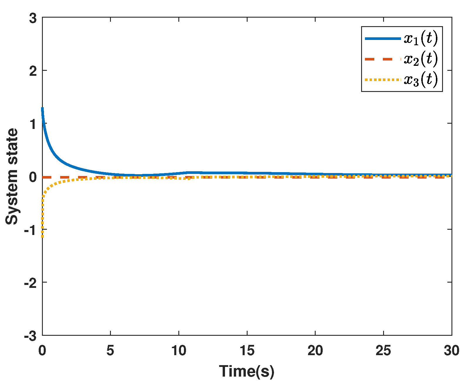
x ( 0 ) = 1.3 0.02 1.1 T ,
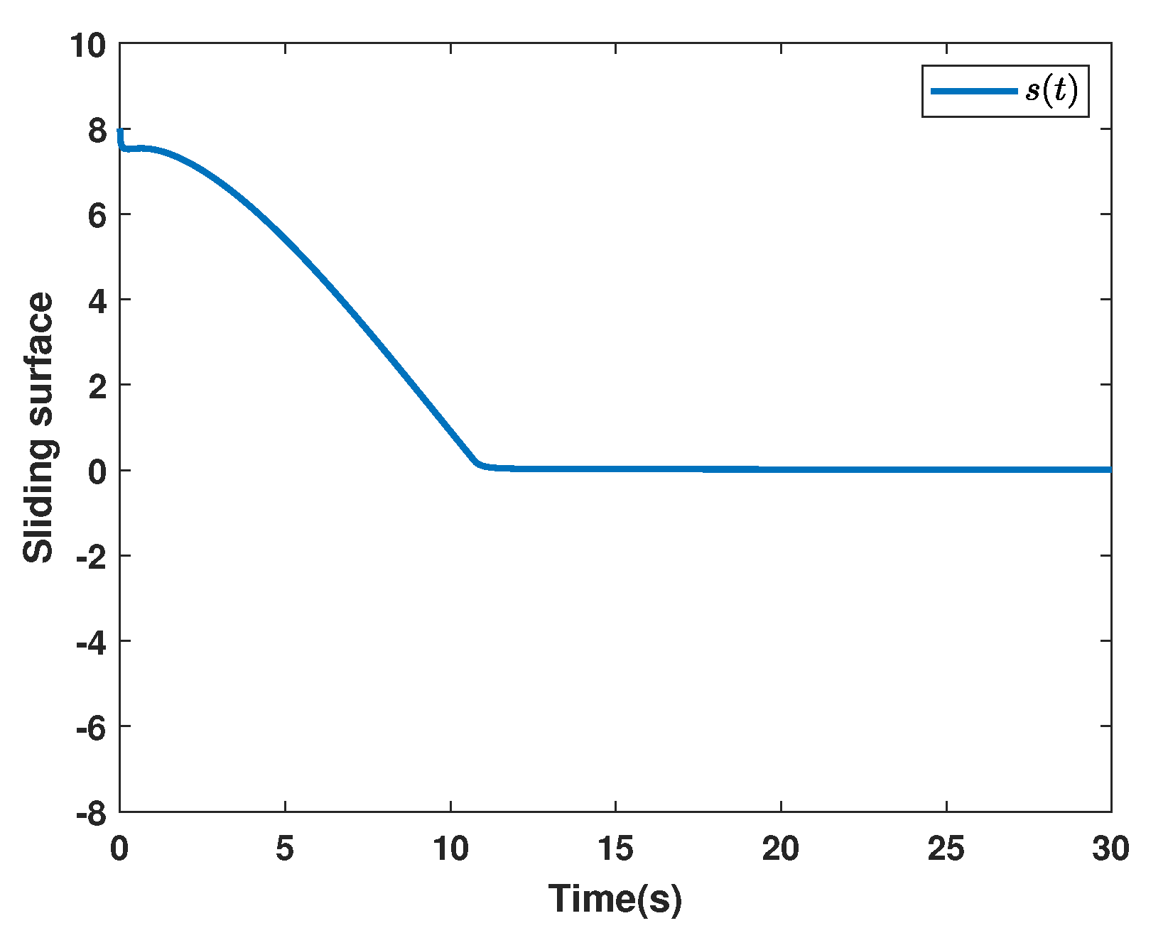
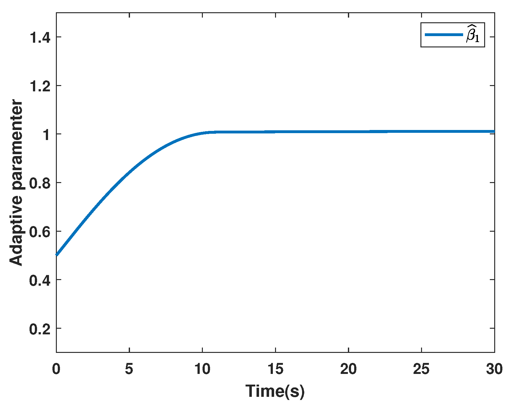
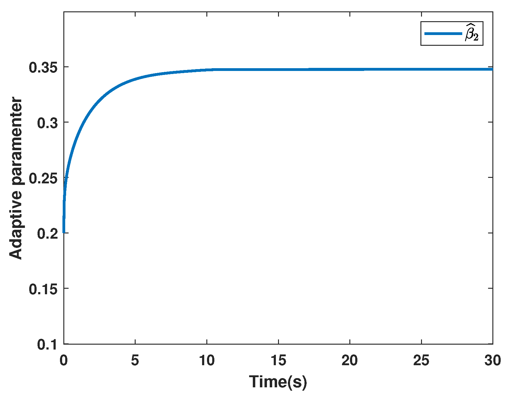
and initial estimates are given as β ^ 1 ( 0 ) = 0.5 , β ^ 2 ( 0 ) = 0.2 . According to the above parameters, we used our method obtain the simulation results. State responses of System (3) are drawn in Figure 3. It reveals that its state x ( t ) converges to zero as t + , and the resulting system is asymptotically stable. Figure 4 denotes the integral-type sliding mode surfaces s ( t ) . Figure 5 plots the control input u ( t ) . The adaptive parameters are shown in Figure 6 and Figure 7.
For comparison, we give the followiing parameters to solve Theorem 4 in [43].
E 0 = 1 0 0 1 1 1 0 0 0 , A 0 = 1 0 1 0 0 0 0 1 1 , A d = 3 5 5 1.5 1 1 3 1 10 B 0 = 1 0 1 ,
B w = 1 1 1 , C 0 = 1.5 2 2.5 , C d = 0.3 0.4 0.5 , U 1 = 0 0 0 1 0 0 T ,
V 1 = 2 4 6 0.1 0.1 0.1 , V 2 = 0.1 0.1 0.1 0 0 0 ,
G = 1 2 5 1 0 0 , D w = 0.2 , d 0 = 0.2 .
According to Theorem 4 in [43] solving LMI (45) of [43], we obtain
t = 0.0570 .
From the result, we could not establish feasibility nor infeasibility. Therefore, the LMI is not strictly feasible.
From the above simulation, we can see that since a X b Y in our method must be invertible, the LMI of our method must have a feasible solution, but E ˜ W T + Z T S T of Theorem 4 in [43] is not necessarily invertible. For example, the LMI in Theorem 4 has no strict feasible solution. We can use the simple MATLAB commands and figures in the Appendix A to show the uncertainty of matrix A and fractional-order model in Example 2.
Example 3.
Considering uncertain SFOSs in System (3).
α = 0.6 ,
C = 0 1 0 1 0 0 , E = 1 1 0 0 1 0 0 0 0 ,
and
A = 3 5 5 1.5 1 1 3 1 10 , B = 1 1 1 ,
U = 1 1 2 T , V = 1 0 2 .
The system uncertainly g ( x ( t ) , t ) is assumed as g ( x ( t ) , t ) = sin ( x 2 ( t ) ) . S 1 and S 2 are chosen as S 1 = 1 1 0 and S 2 = 3 1 1 , respectively. It follows from Equation (9) that
R 1 = 1 0 0 1 , Q = 1 0 0 1 , R 2 = 0 1 0 1 0 0 0 0 1 .
It is found that LMIs (41) and (42) are feasible, and the solutions are
X ¯ = 21.7043 19.1222 3.0762 19.1222 54.7421 4.9304 3.0762 4.9304 35.2072 , Y ¯ = 0 18.8349 3.0762 18.8349 0 4.9304 3.0762 4.9304 0 ,
η = 2.6388 , H = 159.9039 208.8719 .
It follows form L = H R 1 Q ( X ¯ 11 Y ¯ 11 ) 1 Q 1 R 1 1 that
L = 2.7857 25.7836 .
We select the initial condition
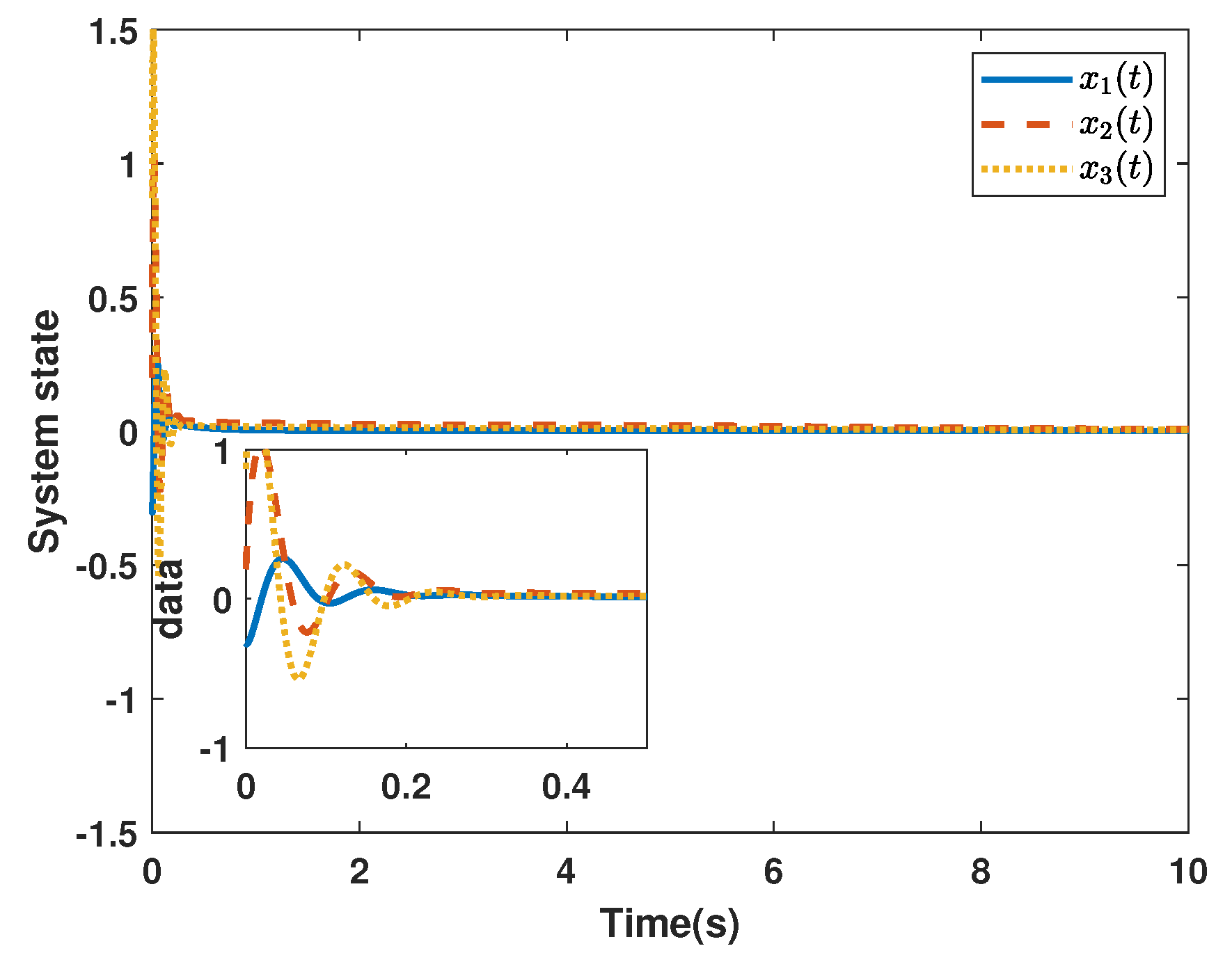
x ( 0 ) = 0.3 0.2 0.02 T ,
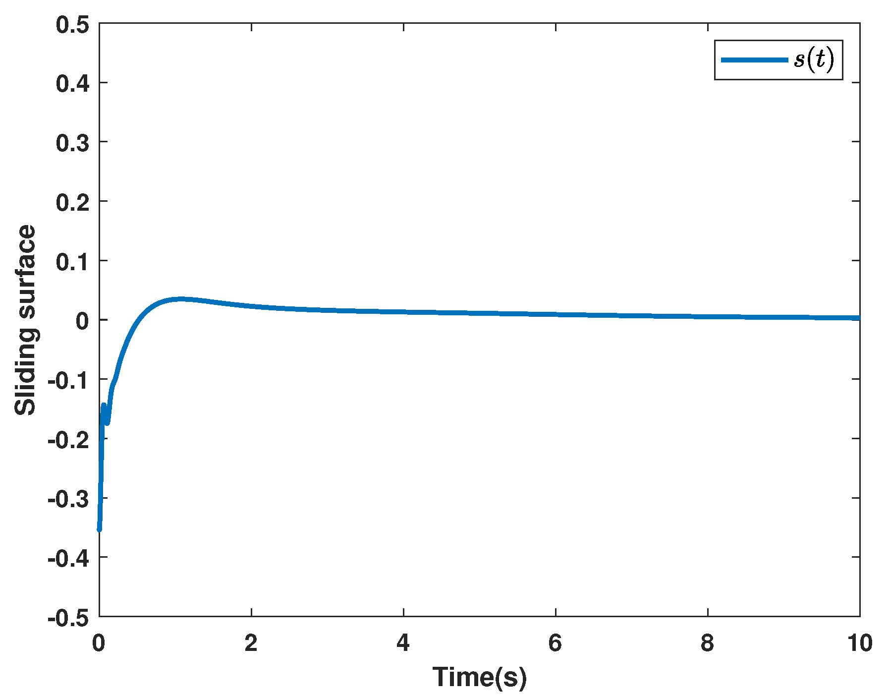
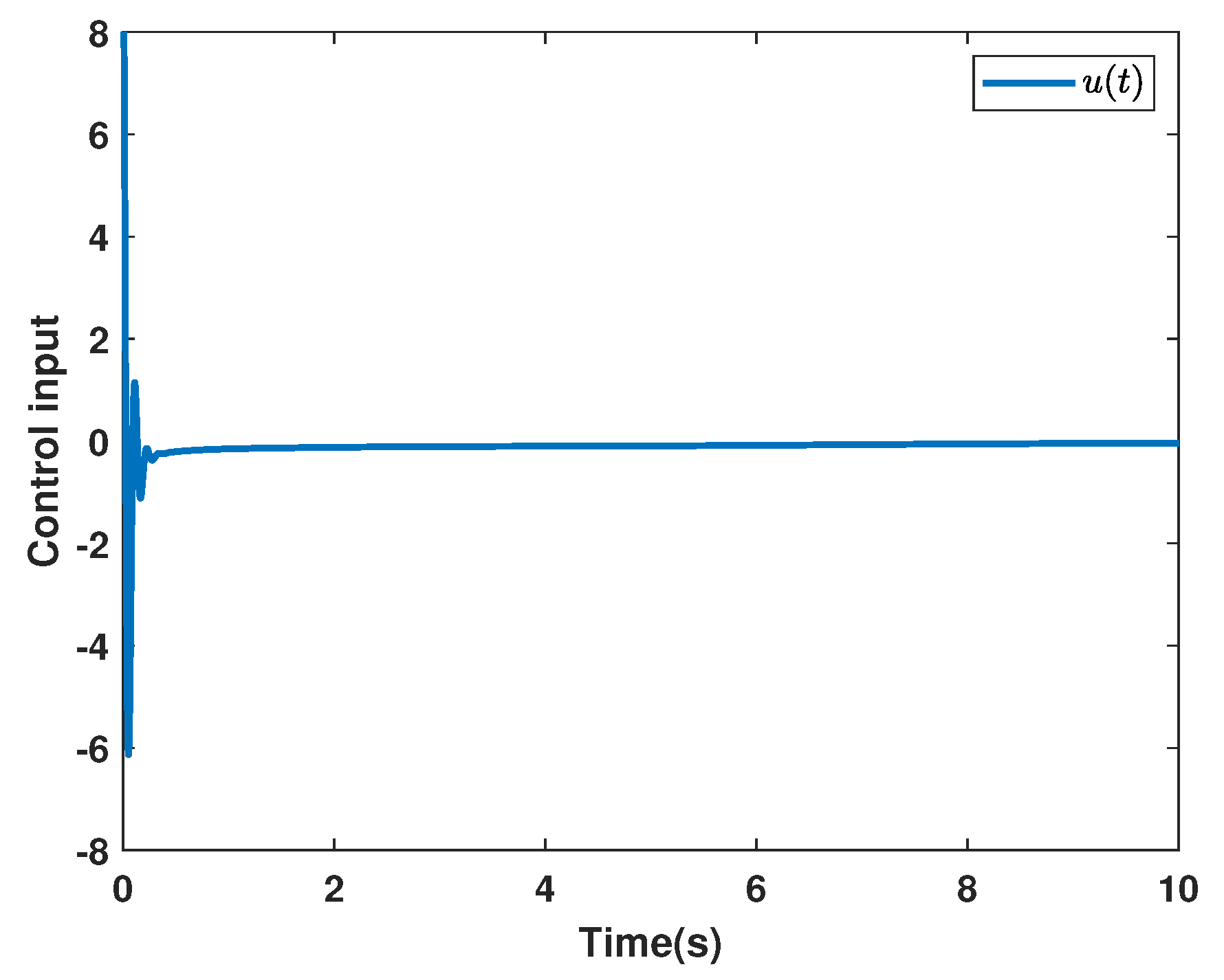
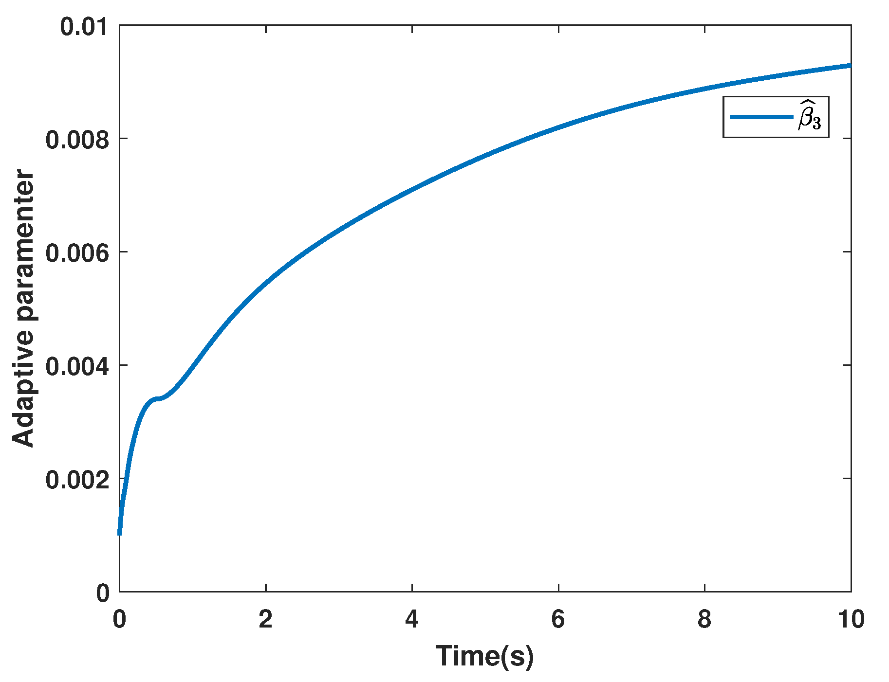
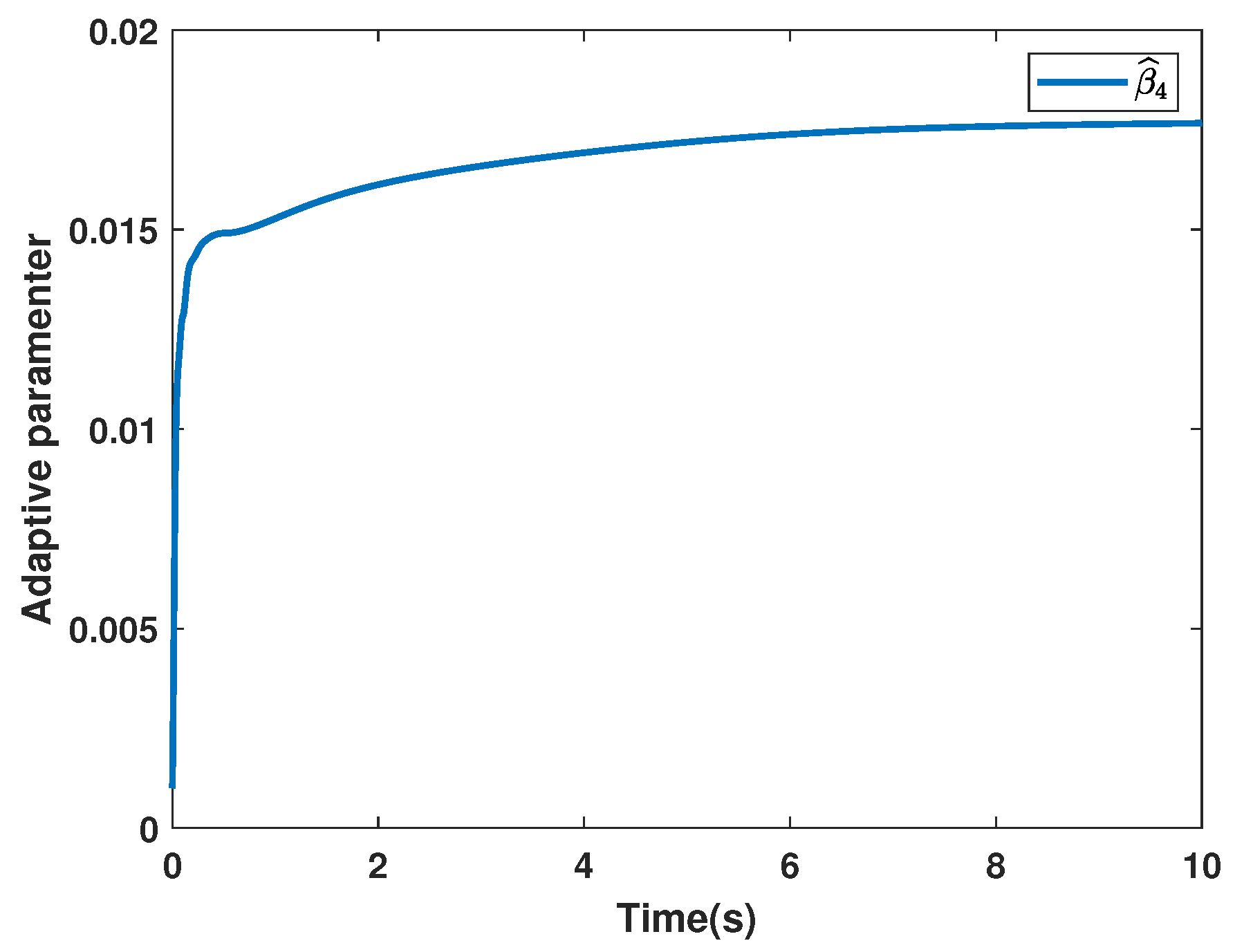
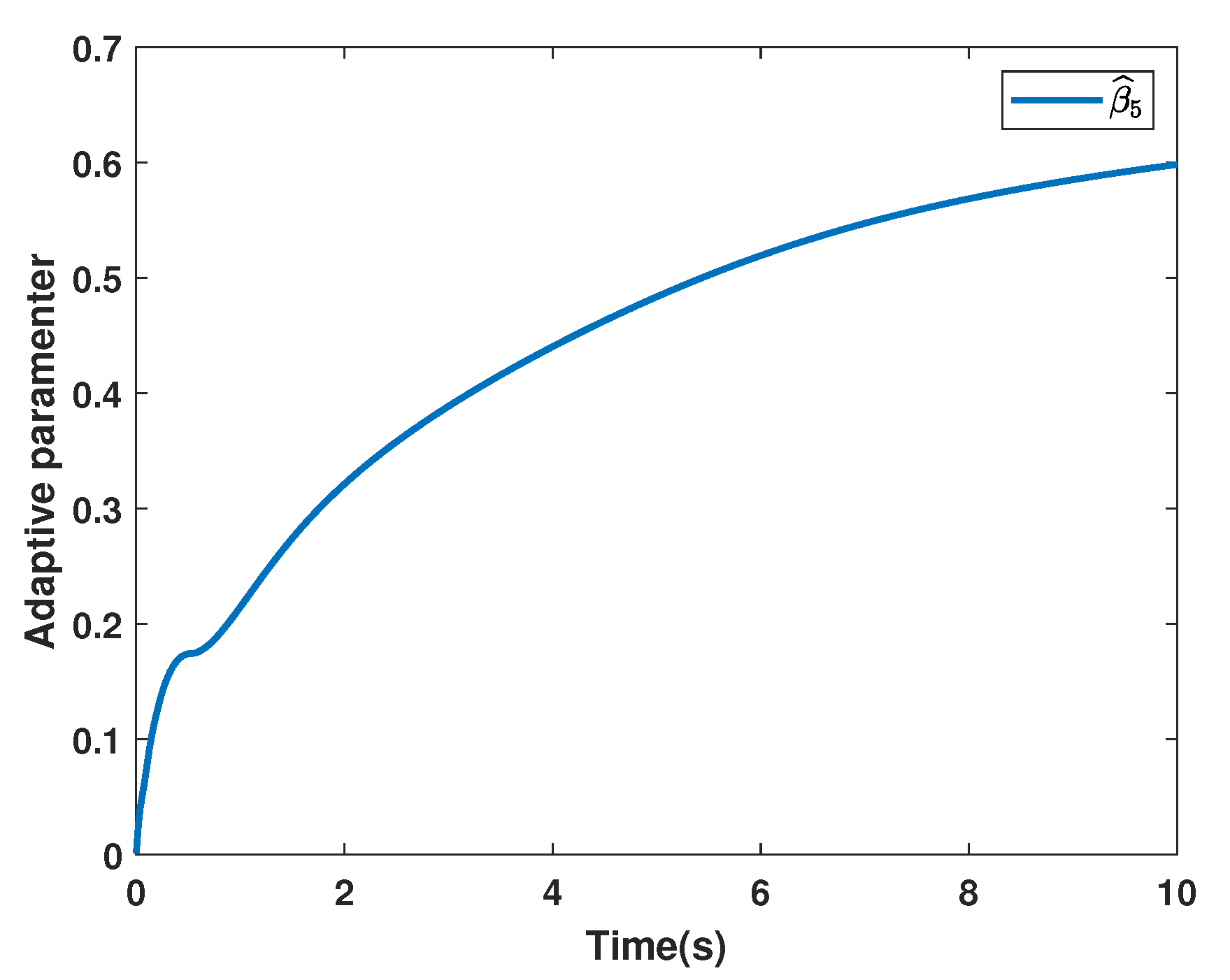
and the initial estimates are given as β ^ 3 ( 0 ) = β ^ 4 ( 0 ) = β ^ 5 ( 0 ) = 0.001 . The system state x ( t ) of System (3) is given in Figure 8. The sliding function s ( t ) is presented in Figure 9, and the control input u ( t ) is shown in Figure 10. The adaptive parameters are depicted in Figure 11, Figure 12 and Figure 13.

5. Conclusions

In this paper, the SMC of SFOSs is studied by means of state feedback and output feedback. By designing a special sliding surface, the sliding motion of the SFOS is a normal FOS, which can be regarded as a new normalization method. A practical example and two numerical examples are utilized to prove the correctness and validity of the conclusions. The adaptive sliding mode design for Takagi-Sugeno fuzzy SFOSs by approximating the neural network is interesting and will be our future research direction.  

Author Contributions

Writing-review and editing, S.C.; Writing-original draft, W.H.; Resources, Q.L. All authors have read and agreed to the published version of the manuscript.

Funding

National key research and development program topic (2020YFB1710003).

Institutional Review Board Statement

Not applicable.

Informed Consent Statement

Not applicable.

Data Availability Statement

Not applicable.

Acknowledgments

Thank Xuefeng Zhang for his guidance and writing help.

Conflicts of Interest

The authors declare no conflict of interest.

Appendix A

Figure A1 shows the part of the simulation of Example 2. The uncertainty of A is given in the MATLAB function module. The code of the main MATLAB function module is given as follows:
  • function dx1 = fcn(x1,x2,x3,s1,u)
  • A = [-1 0 -1;0 0 0;0 -1 -1];
  • B = [1;0;1];
  • V1 = [2 4 6];
  • OO = A+U*s1*V1;
  • dx1 = OO(1,1)*x1+OO(1,2)*x2+OO(1,3)*x3+B(1,1)*(u+x1*sin(x1));
  • where OO represents the uncertainty of matrix A. Figure A2 shows the fractional-order model. Furthermore, Figure A2 shows the fractional module in Figure A1. In the simulation, we can adjust the initial value of the fractional order system by changing the value in the integration module.
Figure A1. Part of the simulation of Example 2.
Fractalfract 06 00253 g0a1
Figure A2. Fractional-order model.
Fractalfract 06 00253 g0a2

References

  1. Magin, R.L. Fractional calculus models of complex dynamics in biological tissues. Comput. Math. Appl. 2010, 59, 1586–1593. [Google Scholar] [CrossRef] [Green Version]
  2. Kaczorek, T. Singular fractional linear systems and electrical circuits. Int. J. Appl. Math. Comput. Sci. 2011, 21, 379–384. [Google Scholar] [CrossRef]
  3. Zhang, X.F.; Huang, W.K. Adaptive neural network sliding mode control for nonlinear singular fractional order systems with mismatched uncertainties. Fractal Fract. 2020, 4, 50. [Google Scholar] [CrossRef]
  4. Li, R.C.; Zhang, Q.L. Robust H sliding mode observer design for a class of Takagi-Sugeno fuzzy descriptor systems with time-varying delay. Appl. Math. Comput. 2018, 337, 158–178. [Google Scholar] [CrossRef]
  5. Boukal, Y.; Darouach, M.; Zasadzinski, M.; Radhy, N.E. Robust H Observer-based control of fractional-order systems with gain parametrization. IEEE Trans. Autom. Control 2017, 62, 5710–5723. [Google Scholar] [CrossRef]
  6. Ibrir, S.; Bettayeb, M. New sufficient conditions for observer-based control of frational order uncertain systems. Automatica 2015, 59, 216–223. [Google Scholar] [CrossRef]
  7. Zhang, X.F.; Lin, C.; Chen, Y.Q.; Boutat, D. A unified framework of stability theorems for LTI fractional order systems with 0<α<2. IEEE Trans. Circuits Syst. II Express Briefs 2020, 67, 3237–3241. [Google Scholar]
  8. Qi, W.H.; Zong, G.D.; Karimi, H.R. Sliding mode control for nonlinear stochastic singular semi-markov jump systems. IEEE Trans. Autom. Control 2019, 65, 361–368. [Google Scholar] [CrossRef]
  9. Wang, Y.Y.; Xie, X.P.; Chadli, M.; Xie, S.R.; Peng, Y. Sliding mode control of fuzzy singularly perturbed descriptor systems. IEEE Trans. Fuzzy Syst. 2020, 29, 2349–2360. [Google Scholar] [CrossRef]
  10. Zhang, X.F.; Dong, J. LMI criteria for admissibility and robust stabilization of singular fractional-order systems possessing poly-topic uncertainties. Fractal Fract. 2020, 4, 58. [Google Scholar] [CrossRef]
  11. N’Doye, I.; Darouach, M.; Zasadzinski, M.; Radhy, N.E. Robust stabilization of uncertain descriptor fractional-order systems. Automatica 2013, 49, 1907–1913. [Google Scholar] [CrossRef]
  12. Wei, Y.; Tse, P.W.; Yao, Z.; Wang, Y. The output feedback control synthesis for a class of singular fractional order systems. ISA Trans. 2017, 69, 1–9. [Google Scholar] [CrossRef] [PubMed]
  13. Meng, B.; Wang, X.H.; Zhang, Z.Y.; Wang, Z. Necessary and sufficient conditions for normalization and sliding mode control of singular fractional-order systems with uncertainties. Sci. China Inf. Sci. 2020, 63, 152202. [Google Scholar] [CrossRef] [Green Version]
  14. Zhang, X.F.; Chen, Y.Q. Admissibility and robust stabilization of continuous linear singular fractional order systems with the fractional order α: The 0<α<1 case. ISA Trans. 2017, 82, 42–50. [Google Scholar] [PubMed]
  15. Zhang, X.F.; Yan, Y.Q. Admissibility of fractional order descriptor systems based on complex variables: An LMI approach. Fractal Fract. 2020, 4, 8. [Google Scholar] [CrossRef] [Green Version]
  16. Marir, S.; Chadli, M.; Bouagada, D. New admissibility conditions for singular linear continuous-time fractional-order systems. J. Frankl. Inst. 2017, 354, 752–766. [Google Scholar] [CrossRef]
  17. Zhang, X.F.; Zhao, Z.L.; Wang, Q.G. Static and dynamic output feedback stabilisation of descriptor fractional order systems. IET Control Theory Appl. 2020, 14, 324–333. [Google Scholar] [CrossRef]
  18. Lin, C.; Chen, B.; Wang, Q.G. Static output feedback stabilization for fractional-order systems in T-S fuzzy models. Neurocomputing 2016, 2016 218, 354–358. [Google Scholar] [CrossRef]
  19. Ji, Y.D.; Su, L.Q.; Qiu, Q. Design of fuzzy output feedback stabilization for uncertain fractional-order systems. Neurocomputing 2016, 173, 1683–1693. [Google Scholar] [CrossRef]
  20. Jiang, J.F.; Li, H.K.; Zhao, K.; Cao, D.Q.; Guirao, J.L. Finite time stability and sliding mode control for uncertain variable fractional order nonlinear systems. Adv. Differ. Equ. 2021, 127. [Google Scholar] [CrossRef]
  21. Feng, Y.; Zhou, M.H.; Zheng, X.M.; Han, F.L.; Yu, X.H. Full-order terminal sliding-mode control of MIMO systems with unmatched uncertainties. J. Frankl. Inst. 2018, 355, 653–674. [Google Scholar] [CrossRef]
  22. Sheng, Y.Z.; Bai, W.J.; Xie, Y.W. Fractional-order (PID)-D-lambda sliding mode control for hypersonic vehicles with neural network disturbance compensator. Nonlinear Dyn. 2021, 103, 849–863. [Google Scholar] [CrossRef]
  23. Jiang, J.F.; Cao, D.Q.; Chen, H.T. Sliding mode control for a class of variable-order fractional chaotic systems. J. Frankl. Inst. 2020, 357, 10127–10158. [Google Scholar] [CrossRef]
  24. Zhan, T.; Liu, X.; Ma, S. A new singular system approach to output feedback sliding mode control for fractional order nonlinear systems. J. Frankl. Inst. 2018, 355, 6746–6762. [Google Scholar] [CrossRef]
  25. Fei, J.T.; Lu, C. Adaptive fractional order sliding mode controller with neural estimator. J. Frankl. Inst. 2018, 355, 2369–2391. [Google Scholar] [CrossRef]
  26. Zhang, J.X.; Yang, G.H. Low-complexity tracking control of strict-feedback systems with unknown control directions. IEEE Trans. Autom. Control 2019, 64, 5175–5182. [Google Scholar] [CrossRef]
  27. Pisano, A.; Rapaić, M.R.; Jelićić, Z.D.; Usai, E. Sliding mode control approaches to the robust regulation of linear multivariable fractional-order dynamics. Int. J. Robust Nonlinear Control 2010, 20, 2045–2056. [Google Scholar] [CrossRef]
  28. Sun, G.; Wu, L.; Kuang, Z.; Ma, Z.; Liu, J. Practical tracking control of linear motor via fractional-order sliding mode. Automatica 2018, 94, 221–235. [Google Scholar] [CrossRef]
  29. Dadras, S.; Momeni, H.R. Control of a fractional-order economical system via sliding mode. Phys. A Stat. Mech. Its Appl. 2010, 389, 2434–2442. [Google Scholar] [CrossRef]
  30. Li, R.C.; Zhang, X.F. Adaptive sliding mode observer design for a class of T-S fuzzy descriptor fractional order systems. IEEE Trans. Fuzzy Syst. 2020, 28, 1951–1960. [Google Scholar] [CrossRef]
  31. Han, H.G.; Wu, X.L.; Qiao, J.F. Design of robust sliding mode control with adaptive reaching Law. IEEE Trans Cybern. 2020, 50, 4415–4424. [Google Scholar] [CrossRef]
  32. Zhang, J.X.; Yang, G.H. Robust adaptive fault-tolerant control for a class of unknown nonlinear systems. IEEE Trans. Ind. Electron. 2017, 64, 585–594. [Google Scholar] [CrossRef]
  33. Sheng, D.; Wei, Y.; Cheng, S.; Wang, Y. Observer-based adaptive backstepping control for fractional order systems with input saturation. ISA Trans. 2018, 82, 18–29. [Google Scholar] [CrossRef] [PubMed]
  34. Zhang, J.X.; Yang, G.H. Fuzzy adaptive output feedback control of uncertain nonlinear systems with prescribed performance. IEEE Trans. Cybern. 2018, 48, 1342–1354. [Google Scholar] [CrossRef] [PubMed]
  35. Bigdeli, N.; Ziazi, H.A. Finite-time fractional-order adaptive intelligent backstepping sliding mode control of uncertain fractional-order chaotic systems. J. Frankl. Inst. 2017, 354, 160–183. [Google Scholar] [CrossRef]
  36. Mirzajani, S.; Aghababa, M.P.; Heydari, A. Adaptive T-S fuzzy control design for fractional-order systems with parametric uncertainty and input constraint. Fuzzy Sets Syst. 2019, 365, 22–39. [Google Scholar] [CrossRef]
  37. Mohammadzadeh, A.; Ghaemi, S. A modified sliding mode approach for synchronization of fractional-order chaotic/hyperchaotic systems by using new self-structuring hierarchical type-2 fuzzy neural network. Neurocomputing 2016, 191, 200–213. [Google Scholar] [CrossRef]
  38. Hosseinnia, S.H.; Ghaderi, R.; Ranjbar, A.N.; Mahmoudian, M.; Momani, S. Sliding mode synchronization of an uncertain fractional order chaotic system. Comput. Math. Appl. 2010, 59, 1637–1643. [Google Scholar] [CrossRef] [Green Version]
  39. Lin, T.C.; Lee, T.Y. Chaos synchronization of uncertain fractional-order chaotic systems with time delay based on adaptive fuzzy sliding mode control. IEEE Trans. Fuzzy Syst. 2011, 19, 623–635. [Google Scholar]
  40. Aghababa, M.P. Design of a chatter-free terminal sliding mode controller for nonlinear fractional-order dynamical systems. Int. J. Control 2013, 86, 1744–1756. [Google Scholar] [CrossRef]
  41. Wang, J.; Shao, C.; Chen, Y.Q. Fractional order sliding mode control via disturbance observer for a class of fractional order systems with mismatched disturbance. Mechatronics 2018, 53, 8–19. [Google Scholar] [CrossRef]
  42. Pashaei, S.; Badamchizadeh, M. A new fractional-order sliding mode controller via a nonlinear disturbance observer for a class of dynamical systems with mismatched disturbances. ISA Trans. 2016, 63, 39–48. [Google Scholar] [CrossRef] [PubMed]
  43. Liu, Q.; Li, R.C.; Zhang, Q.L.; Li, J.X. Adaptive robust H sliding mode control for singular systems with time-varying delay and uncertain derivative matrix. Int. J. Control Autom. Syst. 2019, 17, 3179–3193. [Google Scholar] [CrossRef]
  44. Cuong, H.M.; Dong, H.Q.; Trieu, P.V.; Tuan, L.A. Adaptive fractional-order terminal sliding mode control of rubber-tired gantry cranes with uncertainties and unknown disturbances. Mech. Syst. Signal Process. 2021, 154, 107601. [Google Scholar] [CrossRef]
  45. Tuan, L.A. Neural observer and adaptive fractional-order backstepping fast-terminal sliding-mode control of RTG cranes. IEEE Trans. Ind. Electron. 2021, 68, 434–442. [Google Scholar] [CrossRef]
  46. Van, M.; Ge, S.S.; Ren, H. Finite time fault tolerant control for robot manipulators using time delay estimation and continuous nonsingular fast terminal sliding mode control. IEEE Trans. Cybern. 2017, 47, 1681–1693. [Google Scholar] [CrossRef] [PubMed]
  47. Dassios, I.; Baleanu, D. Caputo and related fractional derivatives in singular systems. Appl. Math. Comput. 2018, 337, 591–606. [Google Scholar] [CrossRef]
Figure 1. Electronic network.
Fractalfract 06 00253 g001
Figure 2. State trajectories of System (3) under the adaptive SMC law.
Fractalfract 06 00253 g002
Figure 3. State trajectories of System (3) under the adaptive SMC law.
Fractalfract 06 00253 g003
Figure 4. Surface function s ( t ) .
Fractalfract 06 00253 g004
Figure 5. Adaptive SMC law u ( t ) .
Fractalfract 06 00253 g005
Figure 6. Adaptive parameter β ^ 1 ( t ) .
Fractalfract 06 00253 g006
Figure 7. Adaptive parameter β ^ 2 ( t ) .
Fractalfract 06 00253 g007
Figure 8. State trajectories of System (1) under the adaptive SMC law.
Fractalfract 06 00253 g008
Figure 9. Surface function s ( t ) .
Fractalfract 06 00253 g009
Figure 10. Adaptive SMC law u ( t ) .
Fractalfract 06 00253 g010
Figure 11. Adaptive parameter β ^ 3 ( t ) .
Fractalfract 06 00253 g011
Figure 12. Adaptive parameter β ^ 4 ( t ) .
Fractalfract 06 00253 g012
Figure 13. Adaptive parameter β ^ 5 ( t ) .
Fractalfract 06 00253 g013
Publisher’s Note: MDPI stays neutral with regard to jurisdictional claims in published maps and institutional affiliations.