Optimal Design of TD-TI Controller for LFC Considering Renewables Penetration by an Improved Chaos Game Optimizer

Abstract

This study presents an innovative strategy for load frequency control (LFC) using a combination structure of tilt-derivative and tilt-integral gains to form a TD-TI controller. Furthermore, a new improved optimization technique, namely the quantum chaos game optimizer (QCGO) is applied to tune the gains of the proposed combination TD-TI controller in two-area interconnected hybrid power systems, while the effectiveness of the proposed QCGO is validated via a comparison of its performance with the traditional CGO and other optimizers when considering 23 bench functions. Correspondingly, the effectiveness of the proposed controller is validated by comparing its performance with other controllers, such as the proportional-integral-derivative (PID) controller based on different optimizers, the tilt-integral-derivative (TID) controller based on a CGO algorithm, and the TID controller based on a QCGO algorithm, where the effectiveness of the proposed TD-TI controller based on the QCGO algorithm is ensured using different load patterns (i.e., step load perturbation (SLP), series SLP, and random load variation (RLV)). Furthermore, the challenges of renewable energy penetration and communication time delay are considered to test the robustness of the proposed controller in achieving more system stability. In addition, the integration of electric vehicles as dispersed energy storage units in both areas has been considered to test their effectiveness in achieving power grid stability. The simulation results elucidate that the proposed TD-TI controller based on the QCGO controller can achieve more system stability under the different aforementioned challenges.

1. Introduction

Recently, the world has become voracious in utilizing electrical power due to the growth of industrial and residential loads. Therefore, it was necessary to establish new electrical power grids to accommodate the load demands. As a result, energy planners were directed to penetrate the renewable energy sources (RESs) with the traditional power grids in the electrical power system to reduce the demerits of these traditional units. In addition, the penetration of RESs with newly established power systems is considered to have an economically good and positive rate that saves in the utilization of the oil, coal, and gas that operate traditional power plants, whereas the resulting flames from burning oil and coal lead to the release of carbon dioxide gas, causing an increase in the ozone hole and an increase in the global warming phenomenon [1]. Although the presence of RESs in electrical power grids reduces the severity of the resulting pollution from the traditional units, these renewable sources suffer from a lack of system inertia. As a result of the reduction in power system inertia caused by renewable sources, the stability and security of the system (i.e., more fluctuations in system frequency) will be affected [2,3]. Moreover, several reasons lead to more frequency fluctuations, such as a mismatching between the generated power and the demand power, system parameter variations, and different sorts of load variations. Hence, the fluctuations in system frequency can be tackled by the LFC [4]. Researchers have done their best to develop several control techniques for achieving reliability in power systems by attaining system frequency and tie-line power flow within tolerable limits.

Many interests have been prompted by researchers to address the issue of LFC in different structures of the power system; (i.e., the single-area power system [5,6], the multi-area interconnected power system [7,8,9,10], and the deregulated power system [11,12]). In addition, several different control techniques have been implemented to overcome the system frequency fluctuations, such as the intelligent control techniques (i.e., fuzzy logic controllers [13], artificial neural networks [14], and adaptive neuro-fuzzy controllers [15]). Moreover, several robust control techniques have been utilized to enhance the power system performance, such as the H-infinite technique [16] and µ-synthesis [17]. Furthermore, optimal control techniques, such as the linear quadratic Gaussian [18] and linear quadratic regulator [19], are implemented to attain the frequency within tolerable limits. In this regard, the majority of the industrial control loop is the proportional-integral-derivative (PID), due to its reputable merits (i.e., simpleness in construction, applicability, functionality, comfort, and inexpensiveness) [20]. Even so, it suffers from a bulky, complicated process when selecting its parameters using trial and error methods. Thus, researchers have been striving to accomplish the optimal PID controller, according to the different optimization techniques utilized in getting the optimal controller parameters. This design of the optimal PID controller leads to ensuring a reliable system performance in comparison to the conventional PID controller when facing the uncertainties in a studied power grid. Accordingly, several optimization techniques have been utilized to fine-tune the optimal PID controller parameters meticulously, including the grasshopper optimization algorithm [21], the ant colony optimization technique [22], the Jaya algorithm [23], and the class topper optimization algorithm [24].

On the other side, the fractional order controllers (FOCs) have become a distinct candidate in power system stabilizing due to their merits (i.e., flexibility in configuration and a higher degree of freedom). The FOCs have several types of poles, such as the hyper-damped poles, that need to be fine-tuned. Accordingly, this leads to an expansion in the stable region, giving more flexibility in the controller design process [25]. Furthermore, there are several types of controllers belonging to the FOC family; the fractional –order-proportional-integral-derivative (FOPID) is one member of this family that has been presented in [26,27]. The FOPID controller has been utilized in several electrical power systems [28,29]. Moreover, the TID controller represents one of the FOCs; it looks exactly like the PID controller in construction except for one difference, which is that the proportional parameter is tilted with a ($1$/${\mathrm{s}}^{\raisebox{1ex}{$1$}\!\left/ \!\raisebox{-1ex}{$\mathrm{n}$}\right.}$) transfer function. This additional transfer function provides the optimization process with better feedback and good tracking performance. Lately, the TID controller has been implemented for solving the LFC problem due to its good merits (i.e., it can change the parameters of the closed-loop system; it has a tremendous ability in disturbance rejection; and it has more reliability with robustness) [30,31]. There is no doubt that fractional calculus provides several options to researchers for creativity and diversity in controller designing. As a result, different engineering problems have been solved by utilizing the amalgamation of the FOPID and TID properties as a hybrid controller [32]. In addition, the researchers’ minds are destined to implement another strategy in control design, which is the cascaded controllers (CCs) form that includes one controller followed by another one; the CCs have more tuning knobs that give better results than in the utilization of non-crude CCs. Thus, many scientific studies have been presented using the different CCs to solve the LFC problem [33,34]. Another construction has been applied while designing different controllers for studying the LFC issue, which depends on the combination of two different controllers to take the benefits of both controllers. There are examples of the combination of different proposed controllers from literature, such as the combination of the model predictive control (MPC) controller with the linear quadratic Gaussian controller [35] and the combination of an adaptive MPC with the recursive polynomial model estimator [36]. Furthermore, a new controller structure, labeled as a feed-forward/feed-backward controller, has been presented to reduce the disadvantages of the PID and TID controllers during system uncertainties that affect the input of the control signal. Thus, many studies have been presented to elucidate the robustness of the feed-forward/feed-backward controller structure in achieving system stability. The integral-proportional-derivative (I-PD) controller and the integral-tilt-derivative (I-TD) controller have been proposed to cope with the LFC problem, achieving more system stability compared to the PID and TID controllers, respectively [37,38].

The achievement of system stability is not dependent on the controller design only, but the utilized optimization technique represents a critical issue that must be selected carefully to attain the optimal controller parameters. Previously, the traditional optimization methods such as the tracking approach [39] and the aggregation methods [40] were applied for regulating the system frequency. In fact, the traditional optimization methods suffer from several drawbacks, such as slump, deathtrap in local minimums, the need for more iterations, and dependence on their initial conditions to attain the optimal solution. So, meta-heuristic optimization techniques such as the artificial bee colony [41], salp swarm algorithm (SSA) [42], and whale optimization algorithm (WOA) [43] have been proposed to overcome all of the previous drawbacks. Though the meta-heuristic optimization algorithms are not usually guaranteed to find the optimal global solution, they can often find a sufficiently good solution in a reasonable time. So, they are an alternative to exhaustive search, which would take exponential time. Moreover, these techniques have several demerits, such as slowing in the rate of convergence, poor local search capability, and local optimum convergence. In this regard, algorithmic scientists have improved these techniques to diminish all of their previous drawbacks. Examples of improved algorithms utilized to achieve system stability are presented as the improved stochastic fractal search algorithm [44] and the sine augmented scaled sine cosine [45]. In this regard, the authors in this work proposed an improved algorithm known as QCGO to select the suggested combining TD-TI controller parameters to attain the optimal studied power grid performance.

Referring to the aforementioned literature related to the LFC issue, there are several control strategies that depend on the designer experience, such as the MPC, the H-infinite techniques, and the fuzzy logic control, that can attain the desired performance, but their parameter-selecting strategies take a long time. In addition, the conventional PID controller has some difficulties when facing system uncertainties. Moreover, several studies have been presented utilizing conventional algorithms and meta-heuristic optimization techniques that have many demerits in comparison to the improved techniques that develop the searching process and obtain the global solution with a few search agents. Furthermore, several previous studies did not consider the different challenges that face power systems (i.e., different types of load variations such as series SLP and RLV, the high penetration of RESs, and communication time delay). According to the above salient observations, this study proposed a new control construction labeled as a combining TD-TI controller that is derived from the form of a TID controller to enhance the studied system stability. The parameters of the proposed combining TD-TI controller can be selected by utilizing the improved algorithm QCGO when considering the challenges of high RESs penetration, different load perturbation types, and communication time delay.

The studied work in this paper is presented to overcome the limitations of the previously published works in the literature.

Table 1. The motivation of current work compared with other published works.

References	[6]	[9]	[28]	[32]	[37]	[38]	This Study
Controller structure	PI/PID controller	PI/PD controller	FOPID/TID controller	Combining of FOPID-TID controller	I-PD controller	I-TD controller	Combining TD-TI controller
Controller design adoption	Firefly algorithm	Backtracking search algorithm	Improved PSO	Manta ray foraging optimization algorithm	Fitness dependent optimizer	Water cycle algorithm	QCGO
Load perturbation challenge	SLP	SLP/RLV	SLP/RLV	SLP/series SLP	SLP	SLP/RLV	SLP/series SLP/RLV
Sort of studied system	Single-area power system	Multi-area power system	Multi-area power system	Multi-area power system	Multi-area power system	Multi-area power system	Multi-area power system
RESs Penetration	Not considered	Not considered	Not considered	considered	Not considered	Not considered	Considered with high penetration
Effect of communication time delay	Not considered	Not considered	Not considered	Not considered	Considered before the action of one control unit only	Not considered	Considered before and after the control action
Effect of EVs	Not considered	Not considered	Not considered	Not considered	Not considered	Not considered	Considered

elucidates the differences between this work and the other published works related to the LFC issue.

The main contributions of this work can be elucidated in detail as follows:

i.

The proposal of a control structure combining TD-TI controllers for LFC of the hybrid two-area interconnected power systems.

ii.

The proposal of a novel technique known as QCGO via improving the quantum mechanics of the CGO algorithm based on the particle swarm optimizer (PSO) to improve the exploration and exploitation strategies of the main CGO algorithm.

iii.

The application of the improved CGO to select the optimal parameters of the proposed controller structure.

iv.

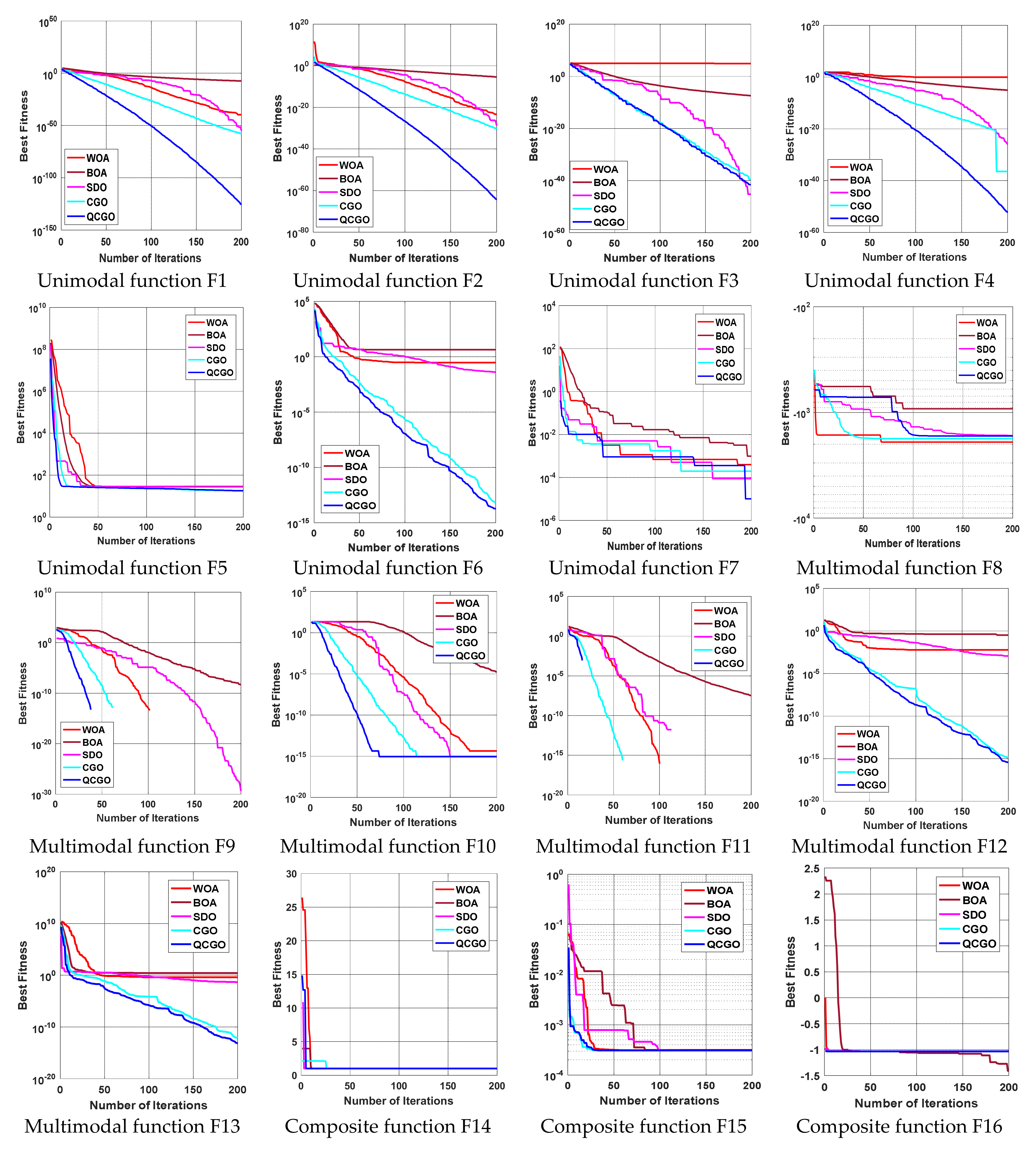
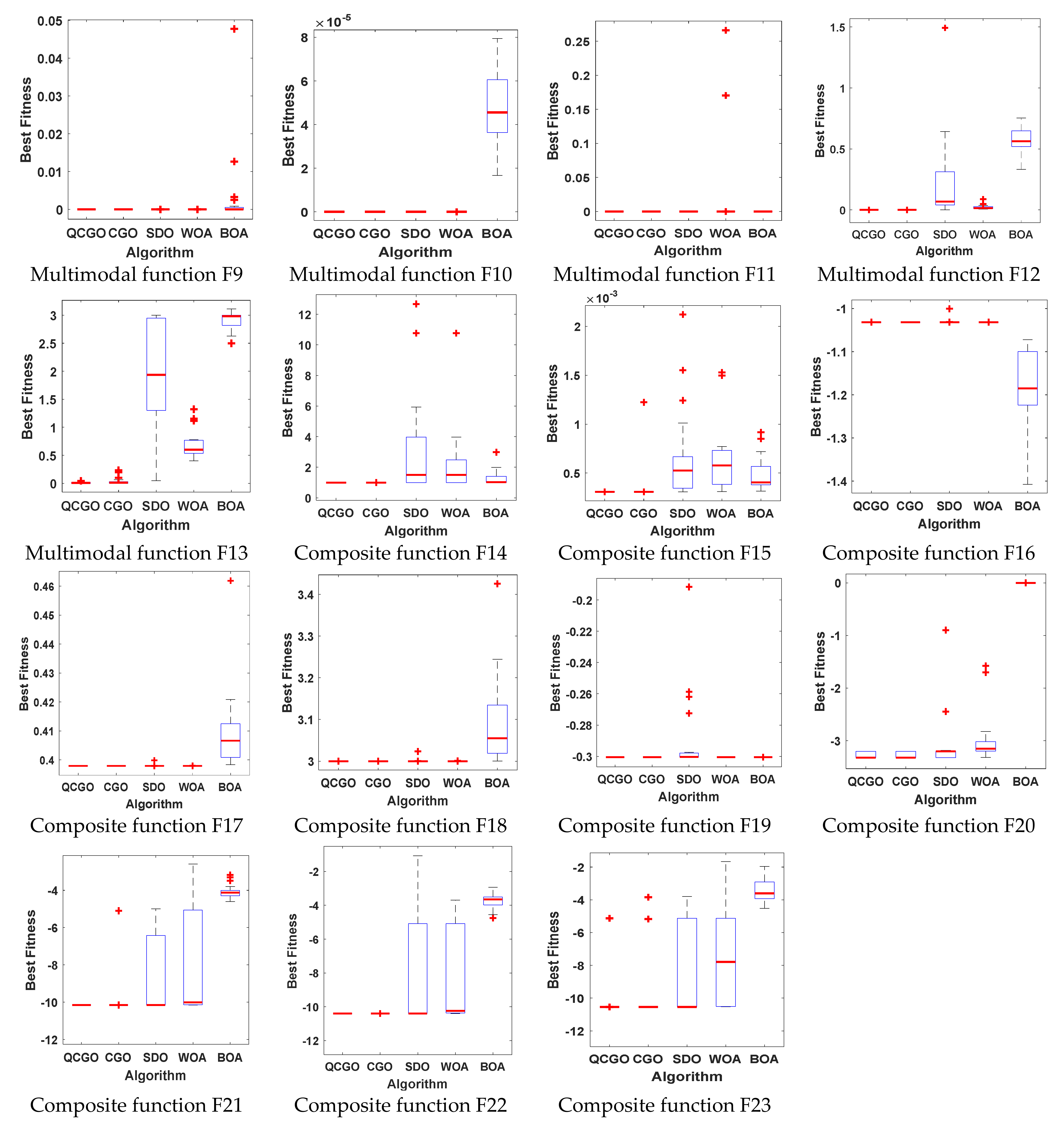
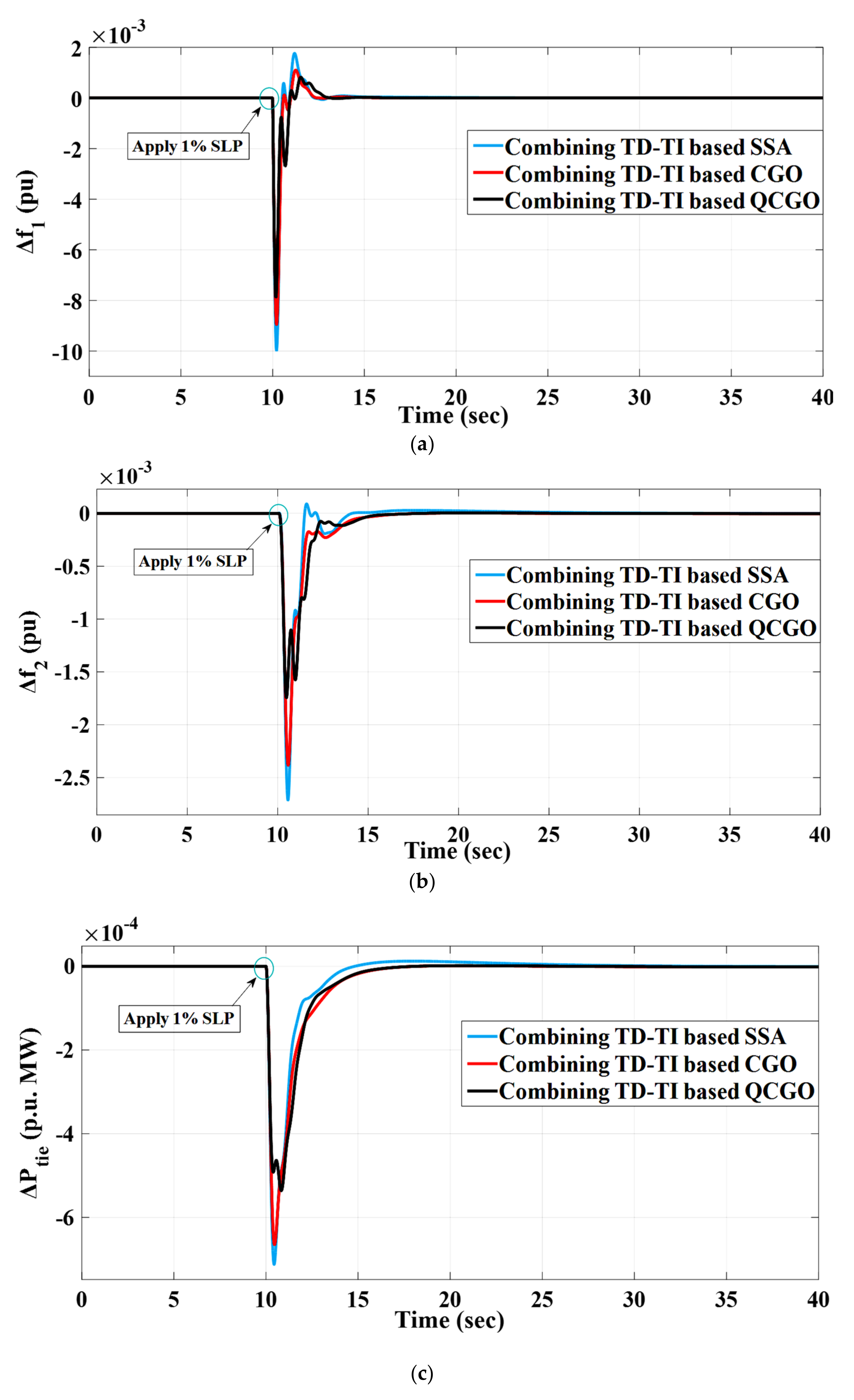
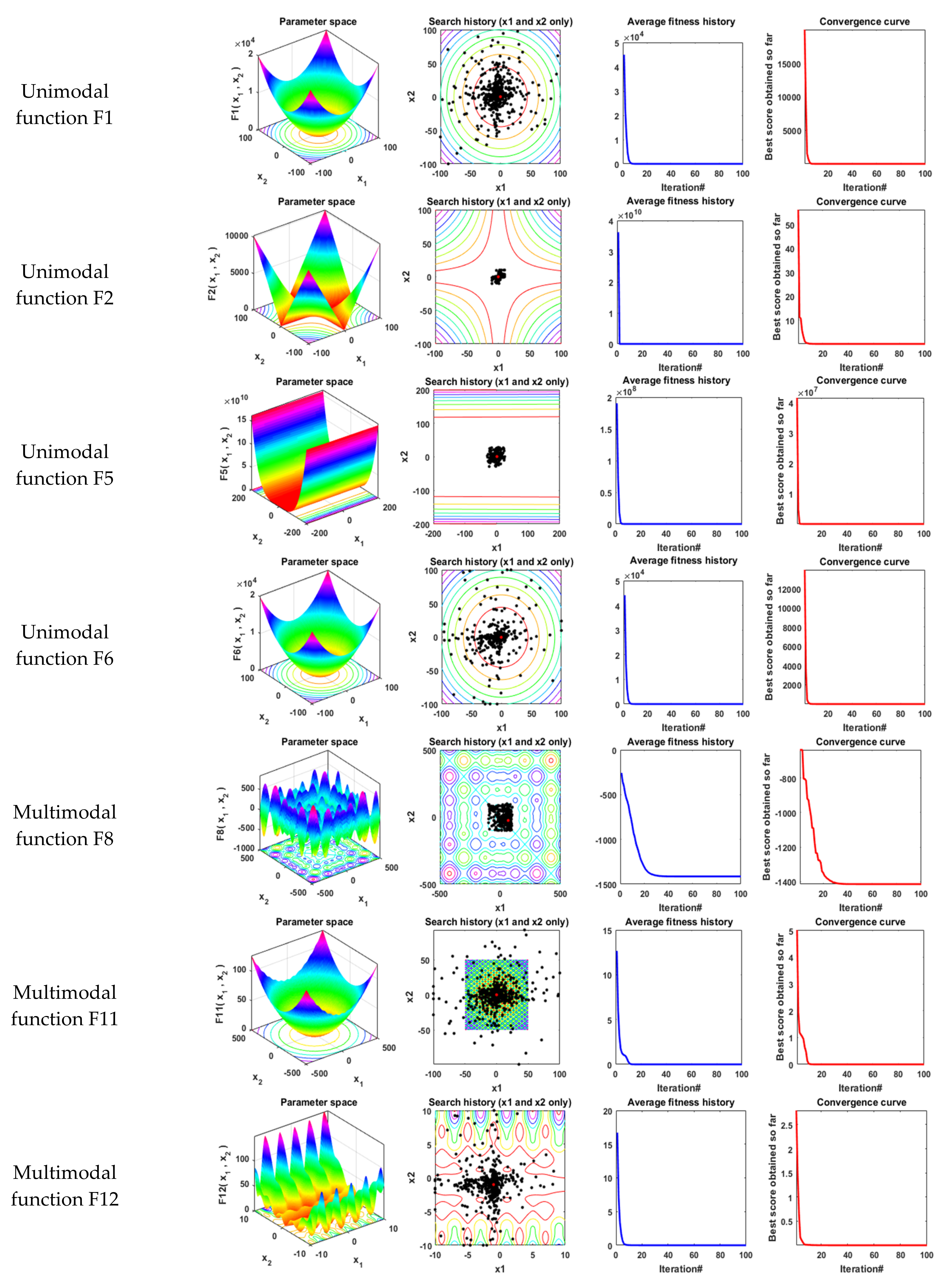
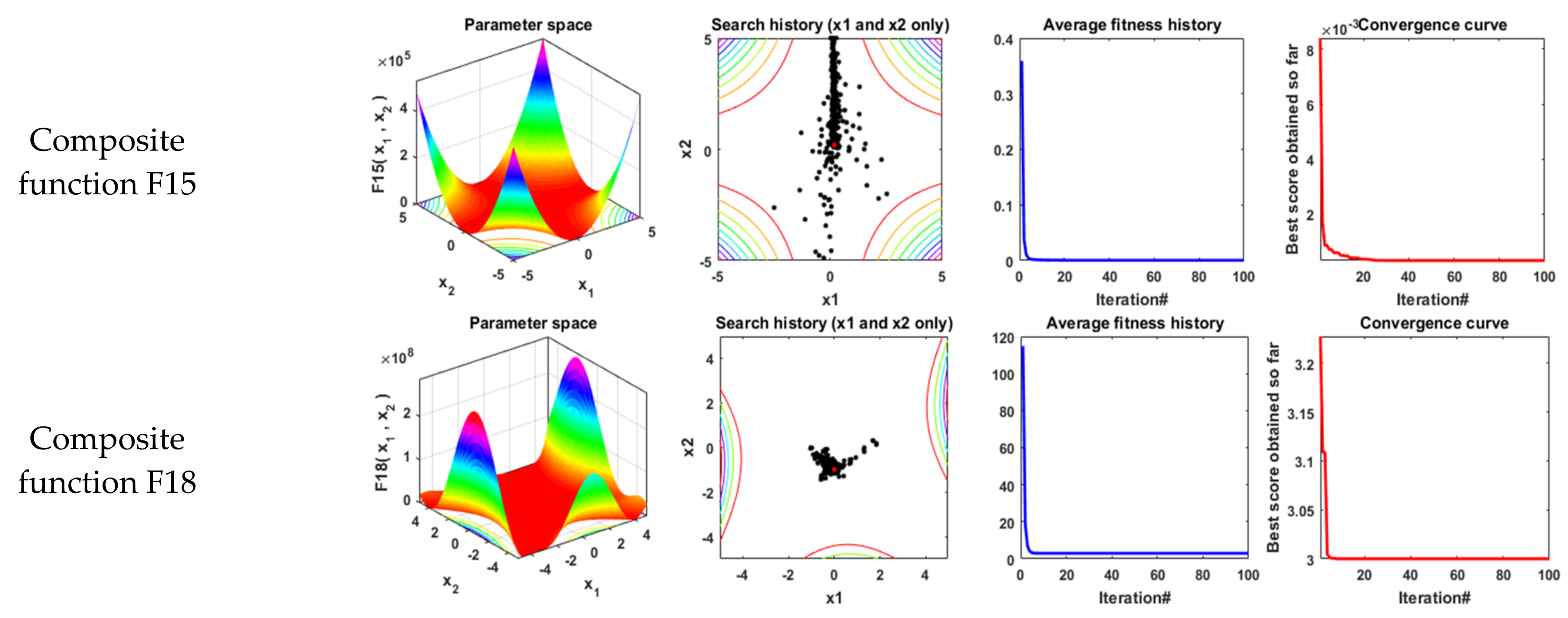
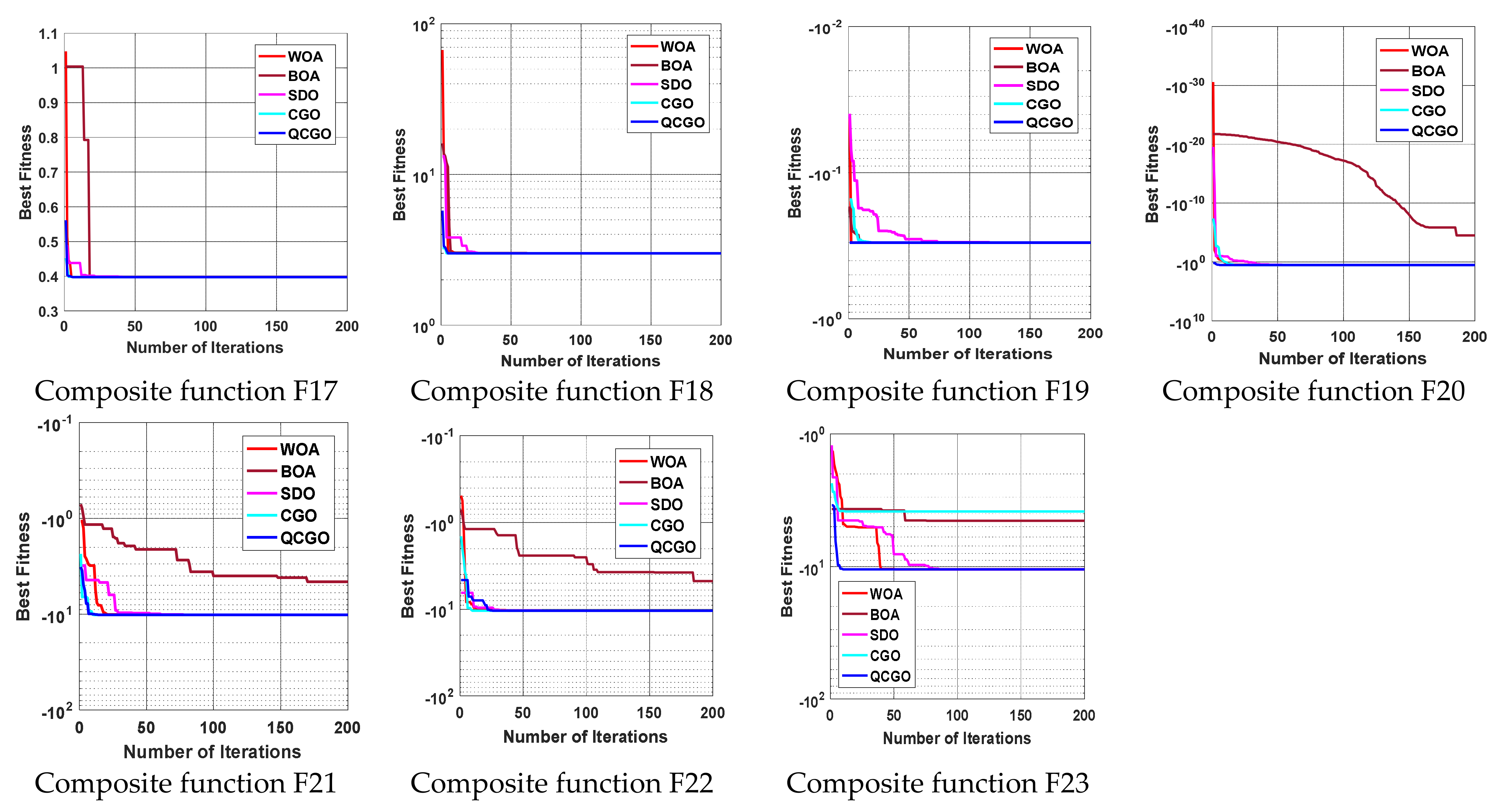
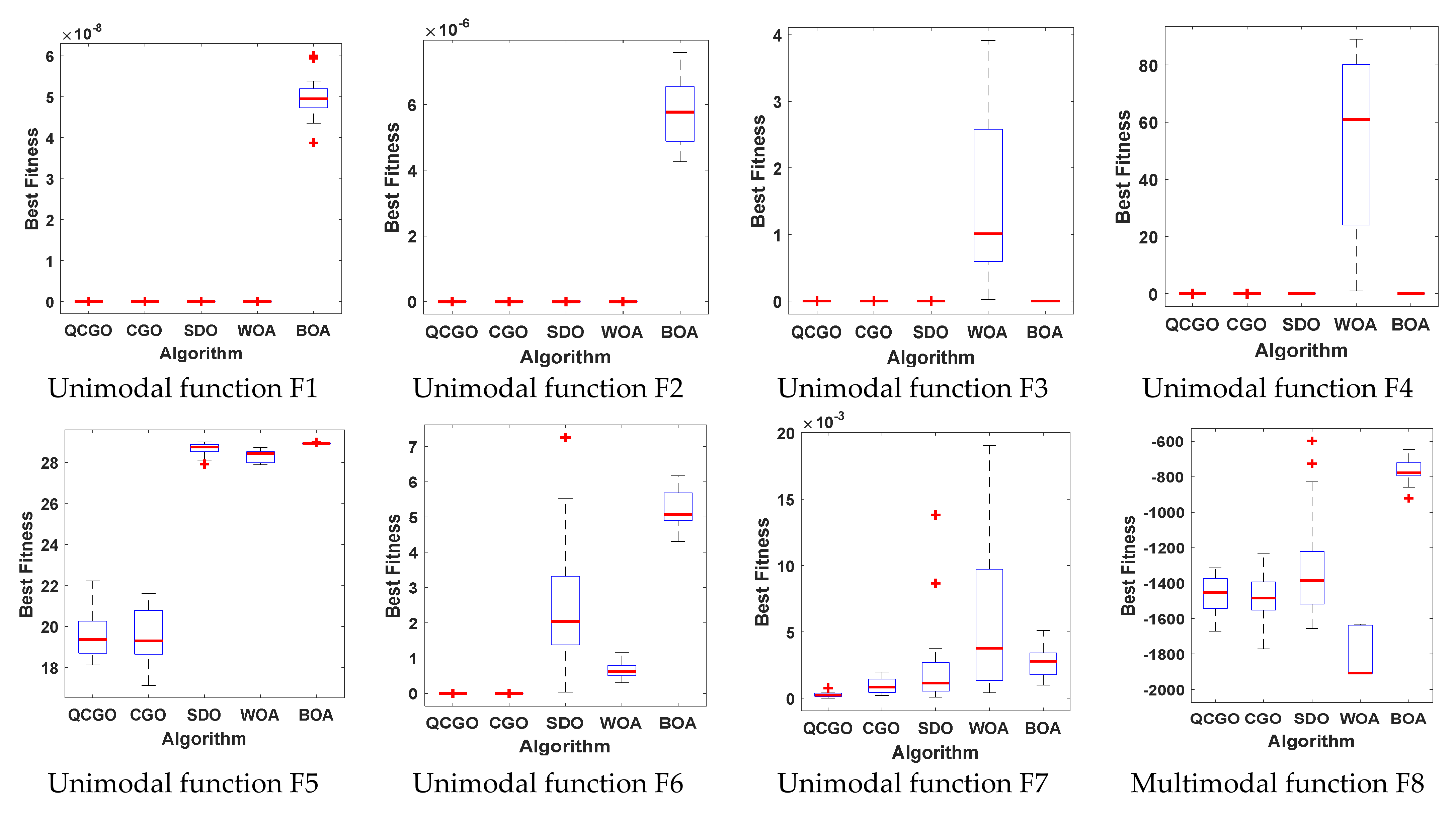
The validation of the performance of the proposed algorithm through a fair-maiden comparison between the proposed QCGO algorithm and other previous techniques (i.e., Supply-demand-based optimization (SDO), WOA, butterfly optimization algorithm (BOA), and the conventional CGO), based on applying 23 bench functions, as well as a fair comparison between the proposed algorithm and other previous algorithms (i.e., CGO, SSA), considering the proposed controller in the multi-area power grid for frequency stability analysis.

v.

The consideration of several challenges, such as the high RESs penetration in both areas, different load perturbation types, and communication time delay to study the system stability state.

vi.

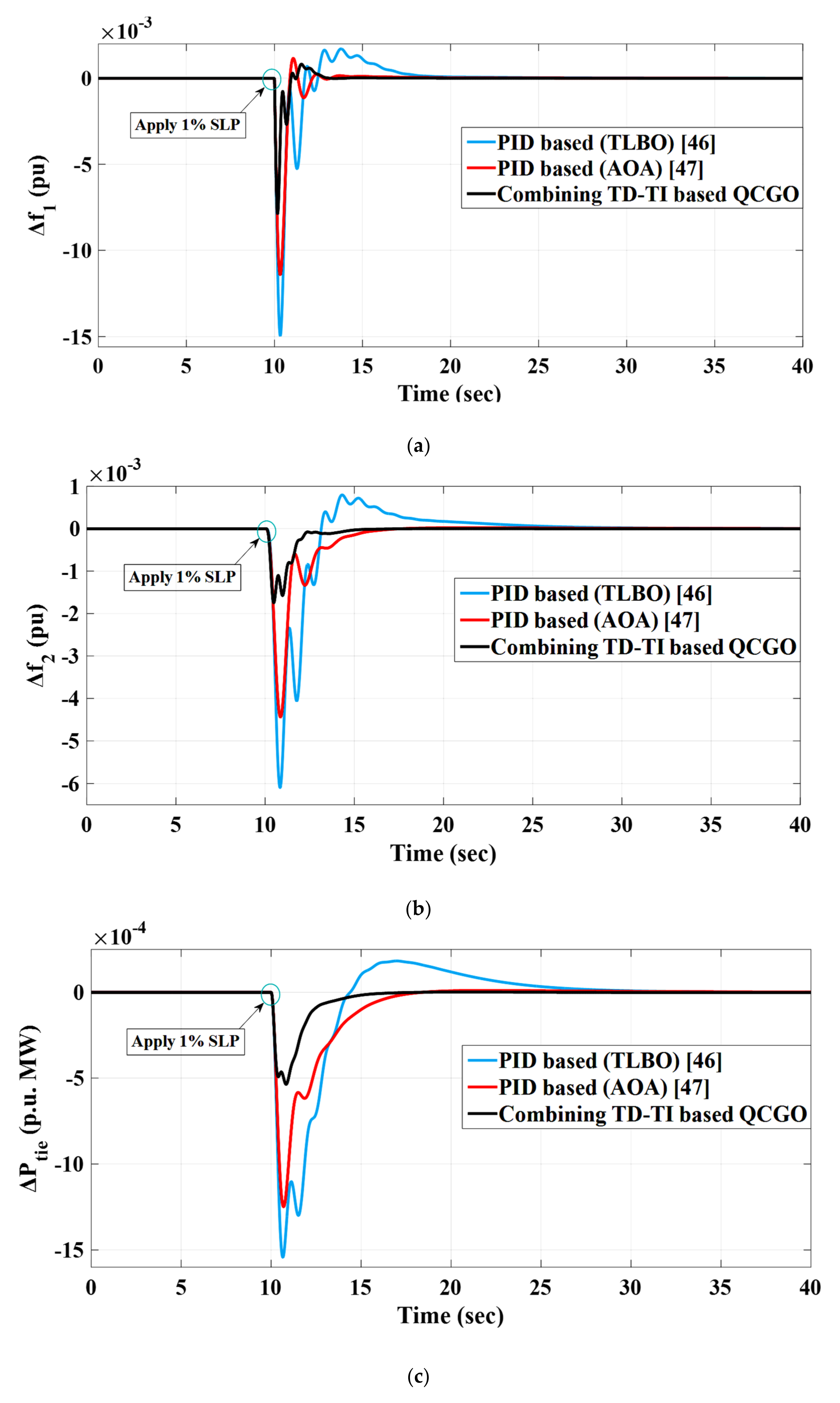
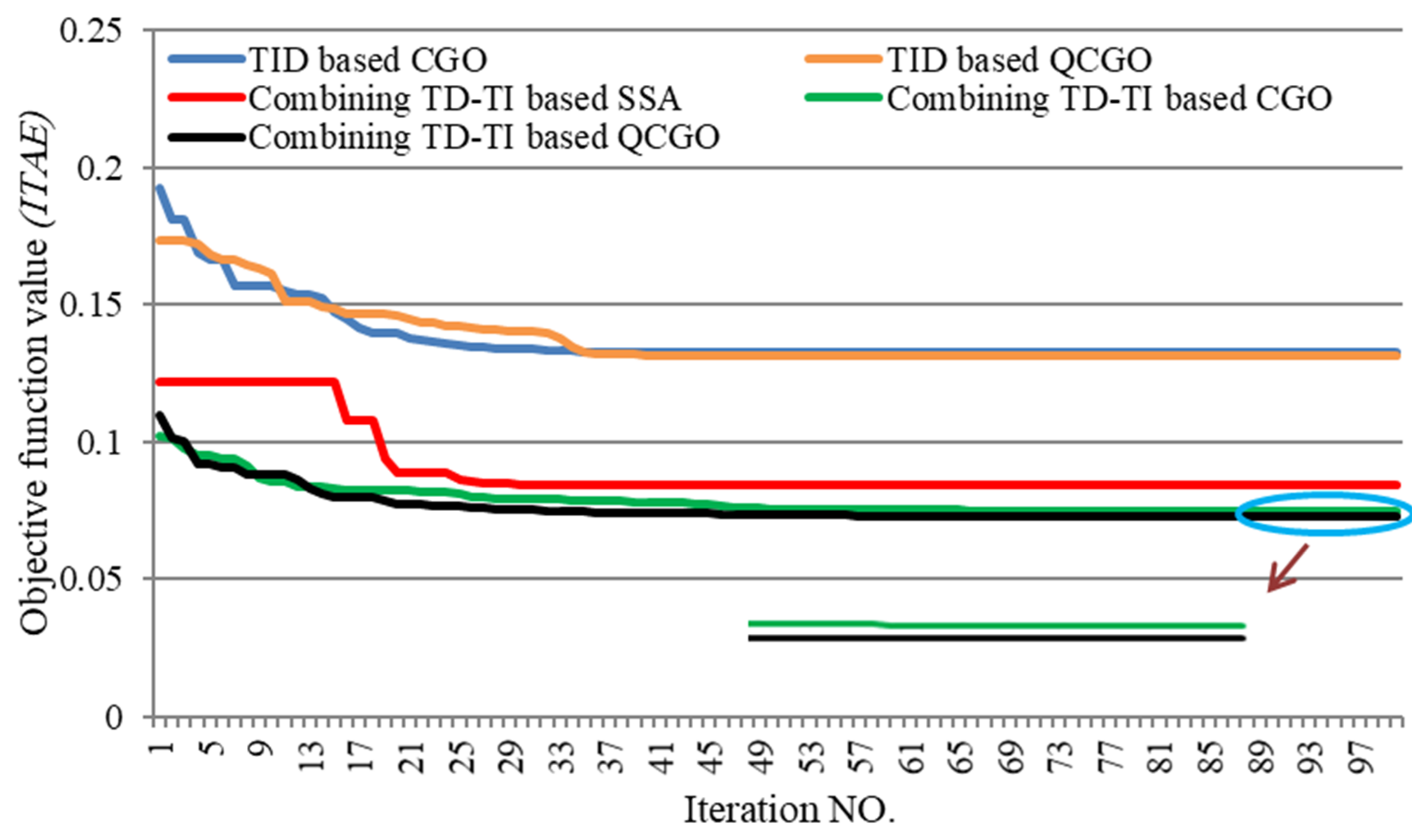
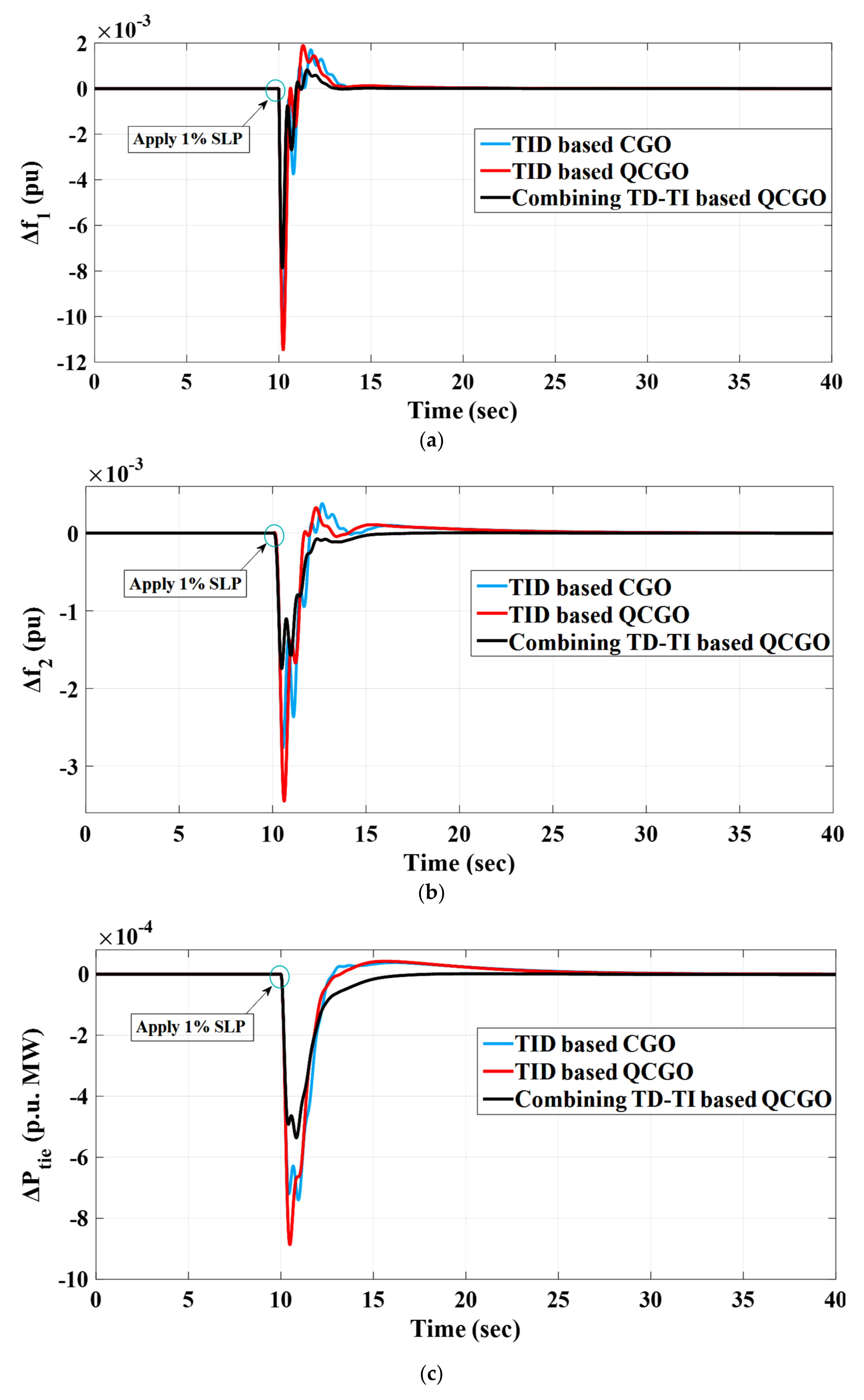
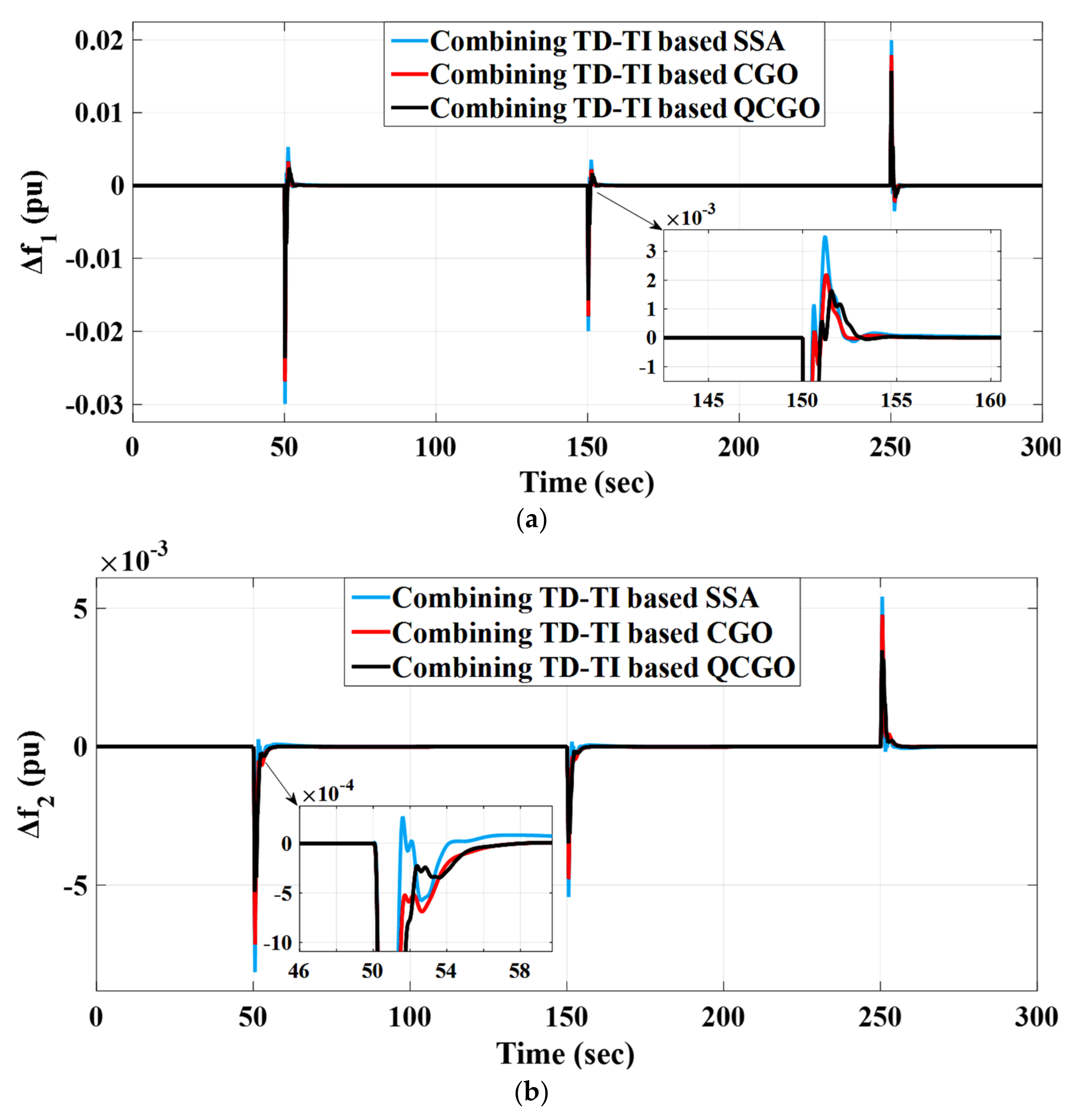
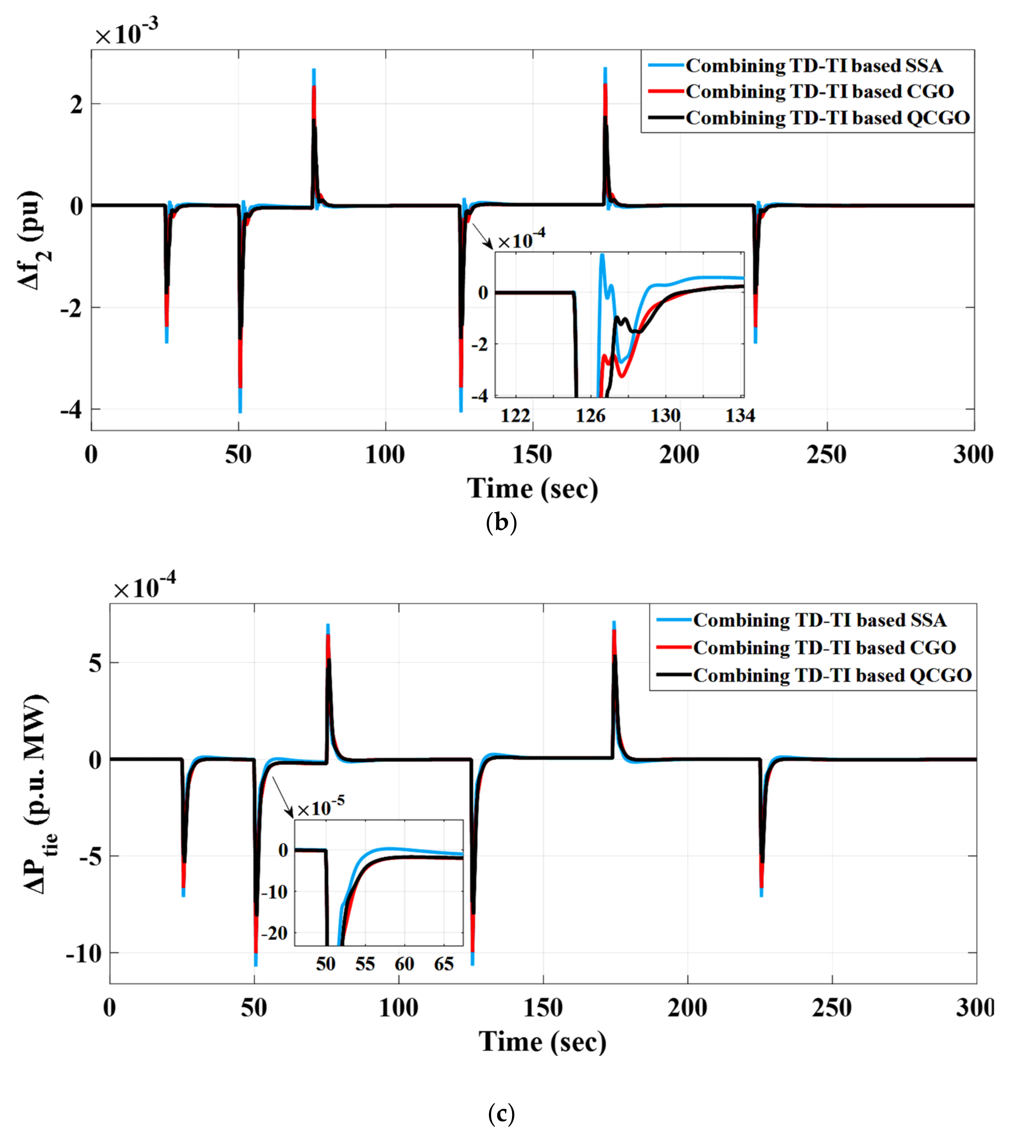
The comparison of the performance of the proposed control TD-TI structure based on QCGO with other available controllers, such as the PID-based teaching learning-based optimization (TLBO) [46]; the PID-based arithmetic optimization algorithm (AOA) [47]; the proposed TD-TI control structure based on CGO; the proposed TD-TI control structure based on SSA; the TID controller based on CGO; and the TID controller based on QCGO, is presented to ensure the effectiveness and robustness of the proposed control structure based on the QCGO algorithm in achieving more system reliability and stability.

vii.

The consideration of the integration of electrical vehicles (EVs) in both areas to support the proposed controller in overcoming the system frequency excursions during high renewables penetration.

The remainder of this article is organized into several sections that are clarified as follows: the studied system topology which considers the high penetration of RESs and EVs is illustrated in Section 2. Section 3 discusses the proposed control approach and the formulation of the studied problem. Then, the procedure of the improved QCGO technique is given in Section 4. Moreover, the simulation results according to the different scenarios are clarified in Section 5. Finally, Section 6 summarizes the conclusions of the current work.

2. The Studied System Topology

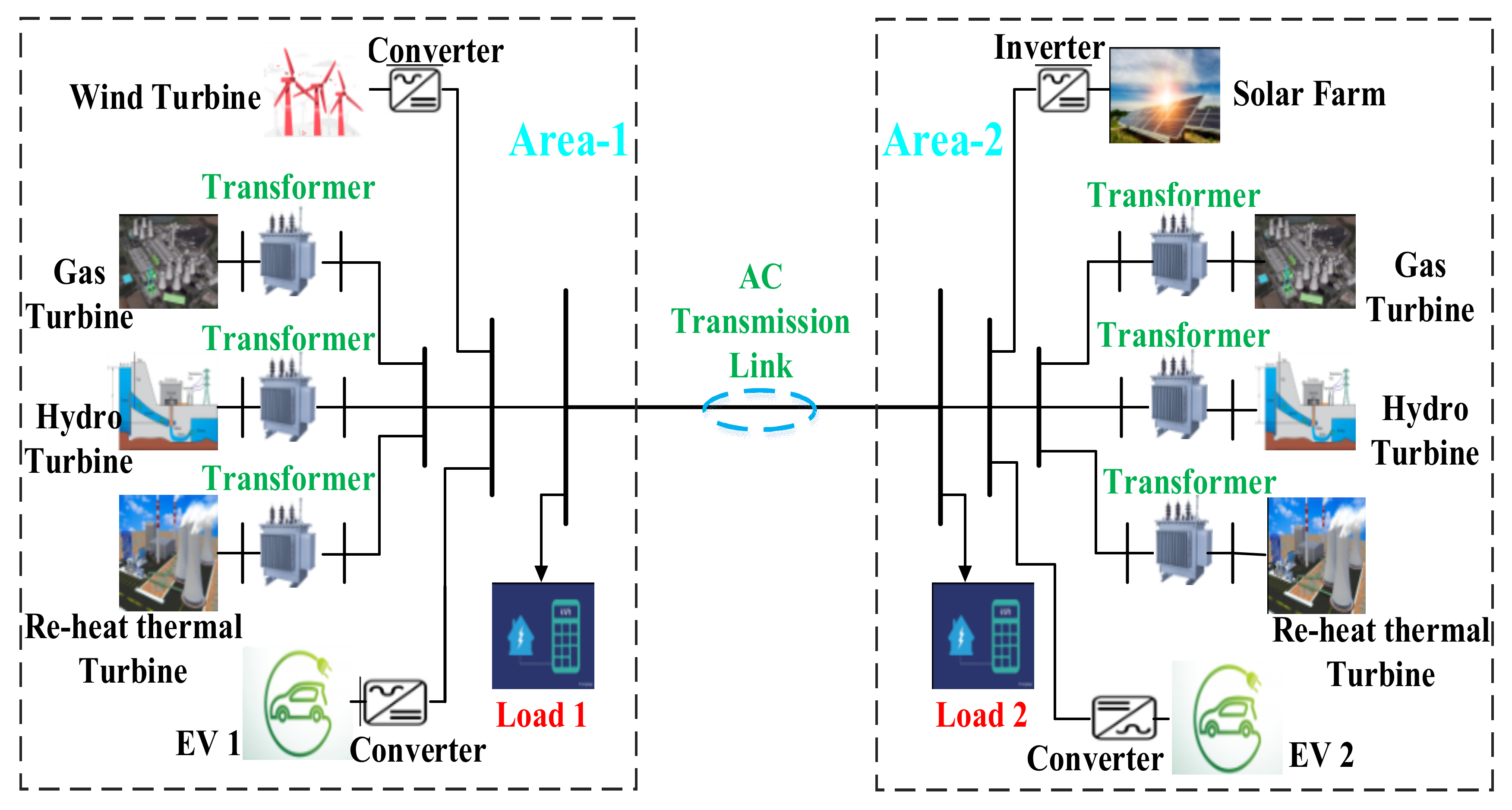
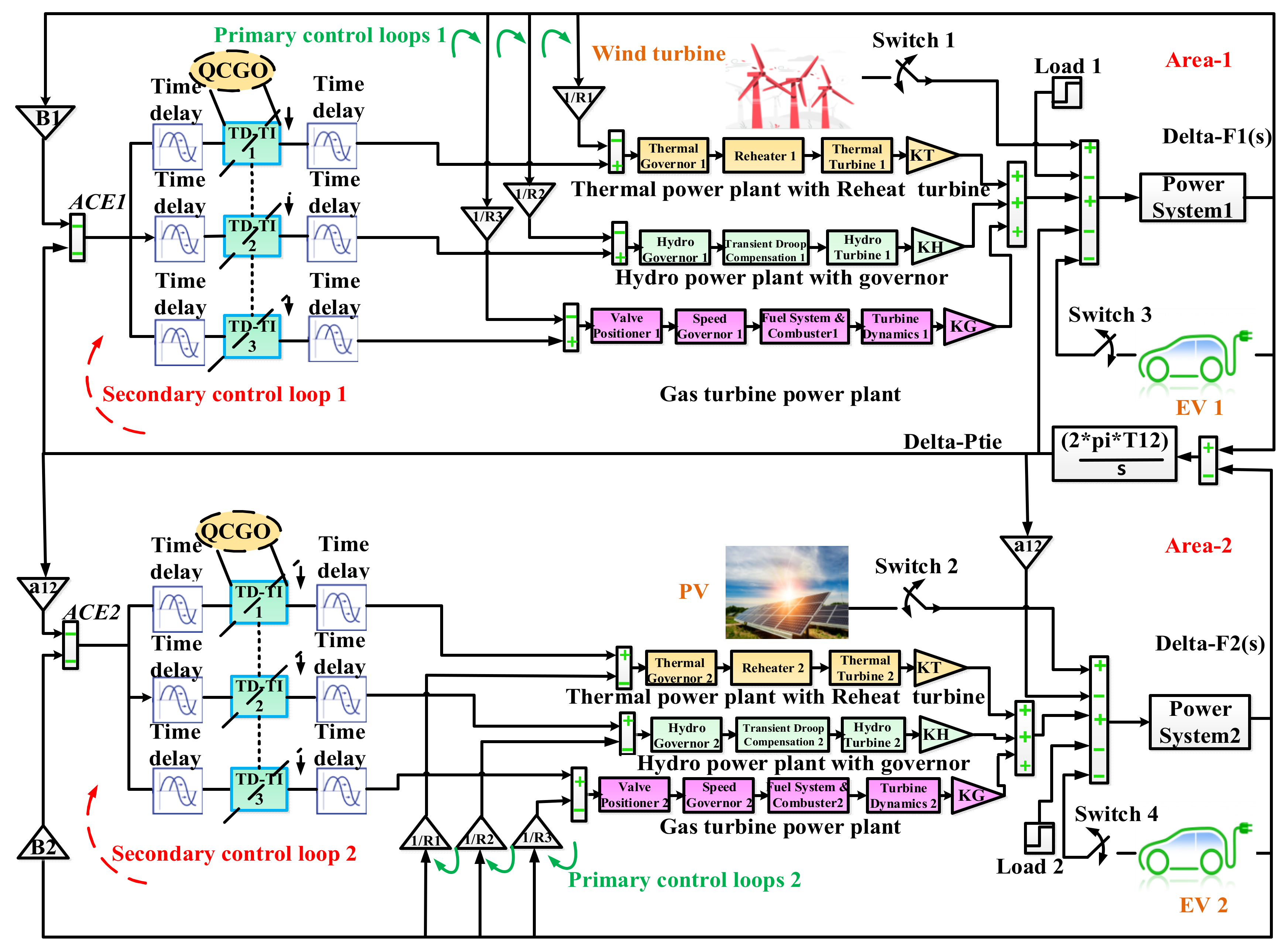
2.1. Two-Area Interconnected Hybrid Power Grid Configuration

In this article, the issue of LFC related to electrical power grids has been addressed by conducting a study on two-area interconnected hybrid power systems. The studied power grid encompasses two interconnected areas, which include several conventional generation power plants, such as the thermal unit, hydropower unit, and gas unit. The capacity of each area in the studied power grid that includes the three traditional units (i.e., thermal, hydro, and gas) is 2000 MW of rated power [48], of which the largest percentage of electrical power sharing went to the thermal power plant, which contributes 1087 MW, then the hydropower plant, which contributes 653 MW, and the gas turbine, sharing the generated power with 262 MW. The investigated power grid is presented as a simplified model shown in Figure 1.

Figure 2 shows the block diagram of the studied two-area interconnected hybrid power grid. The transfer functions in the studied power grid are listed in

Table 2. The transfer functions that are presented in the studied power grid.

Control Block	Transfer Functions
Thermal Governor	$\frac{1}{T_{sg}·\mathrm{s}+1}$
Reheater of Thermal Turbine	$\frac{K_r·T_r·\mathrm{s}+1}{T_r·\mathrm{s}+1}$
Thermal Turbine	$\frac{1}{T_t·\mathrm{s}+1}$
Hydro Governor	$\frac{1}{T_{gh}·\mathrm{s}+1}$
Transient Droop Compensation	$\frac{T_{rs}·\mathrm{s}+1}{T_{rh}·\mathrm{s}+1}$
Hydro Turbine	$\frac{-T_w·\mathrm{s}+1}{0.5T_w·\mathrm{s}+1}$
Valve Positioner of Gas Turbine	$\frac{1}{b_g·\mathrm{s}+c_g}$
Speed Governor of Gas Turbine	$\frac{x_c·\mathrm{s}+1}{Y_c·\mathrm{s}+1}$
Fuel System and Combustor	$\frac{T_{cr}·\mathrm{s}+1}{T_{fc}·\mathrm{s}+1}$
Gas Turbine Dynamics	$\frac{1}{T_{cd}·\mathrm{s}+1}$
Power System 1	$\frac{K_{ps1}}{T_{ps1}·\mathrm{s}+1}$
Power System 2	$\frac{K_{ps2}}{T_{ps2}·\mathrm{s}+1}$
Electrical Vehicle 1	$\frac{K_{EV1}}{T_{EV1}·\mathrm{s}+1}$
Electrical Vehicle 2	$\frac{K_{EV2}}{T_{EV2}·\mathrm{s}+1}$

. The amalgamation of the TD-TI controller is proposed to be equipped in both areas for each generation unit to minimize the oscillations in the frequencies of both areas and the tie-line power flow between them. The attitude of the input signal of the proposed combining TD-TI controller can be represented as the ACE, while the attitude of the output signal can be represented as the action of the secondary/supplementary control on each generation power plant, in order to obtain extra active power for enhancing the power grid performance.

Table 3. The standard parameter values of the two interconnected identical areas [47].

Parameter Descriptions	Symbol	Standard Values
Frequency bias factor	$B_i$	0.4312 MW/Hz
Coefficient of synchronizing	$T_{12}$	0.0433 MW
The regulation constant of thermal turbine The regulation constant of hydropower plant The regulation constant of gas turbine	$R_1$ $R_2$ $R_3$	2.4 HZ/MW 2.4 HZ/MW 2.4 HZ/MW
Control area capacity ratio	$a_{12}$	−1
Participation factor for a thermal unit	$K_T$	0.543478
Participation factor for a hydro unit	$K_H$	0.326084
Participation factor for a gas unit	$K_G$	0.130438
Gain constant of power system	$K_{ps}$	68.9566
The time constant of the power system	$T_{ps}$	11.49 s
Governor time constant	$T_{sg}$	0.08 s
Turbine time constant	$T_t$	0.3 s
Gain of reheater steam turbine	$K_r$	0.3
The time constant of reheater steam turbine	$T_r$	10 s
Speed governor time constant of hydro turbine	$T_{gh}$	0.2 s
Speed governor reset time of the hydro turbine	$T_{rs}$	5 s
The transient droop time constant of hydro turbine speed governor	$T_{rh}$	28.75 s
Nominal string time of water in penstock	$T_w$	1 s
Gas turbine constant of valve positioner	$b_g$	0.05
Valve positioner of gas turbine	$c_g$	1
The lag time constant of the gas turbine speed governor	$Y_c$	1 s
The lead time constant of the gas turbine speed governor	$X_c$	0.6 s
Gas turbine combustion reaction time delay	$T_{cr}$	0.01 s
Gas turbine fuel time constant	$T_{fc}$	0.23 s
Gas turbine compressor discharge volume–time constant	$T_{cd}$	0.2 s
Gain of electrical vehicle	$K_{EV}$	1
The time constant of electrical vehicle	$T_{EV}$	0.28 s

elucidates all the parameters included in the studied power grid with their nominal values. The ACEs in both areas can be obtained according to the formulas that follow in Equations (1) and (2) [47]:

$$AC{E}_1=\Delta {\mathrm{C}}_{\mathrm{tie}1-2}+B_1\Delta {\mathrm{i}}_1$$

(1)

$$AC{E}_2=\Delta {\mathrm{C}}_{\mathrm{tie}2-1}+B_2\Delta {\mathrm{i}}_2$$

(2)

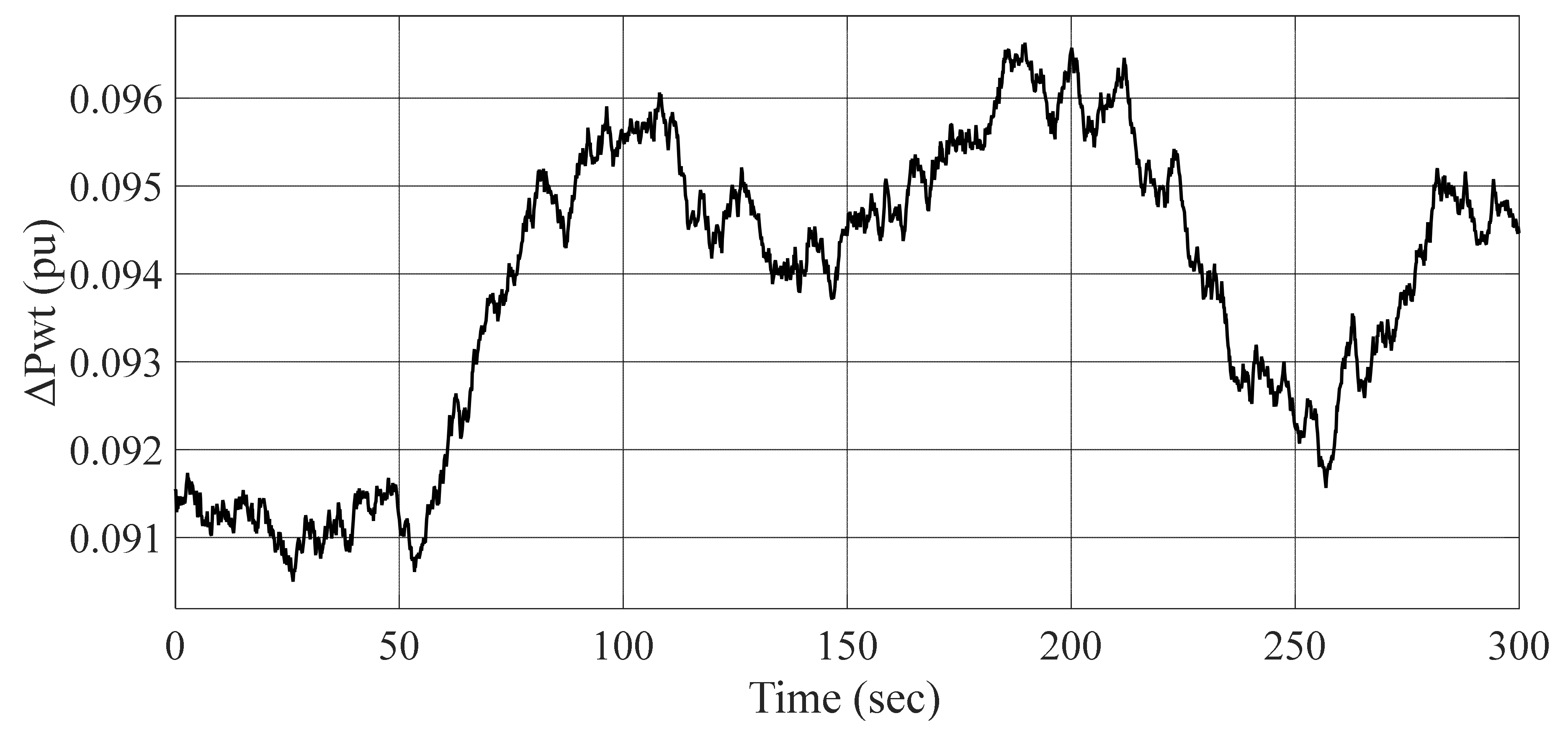
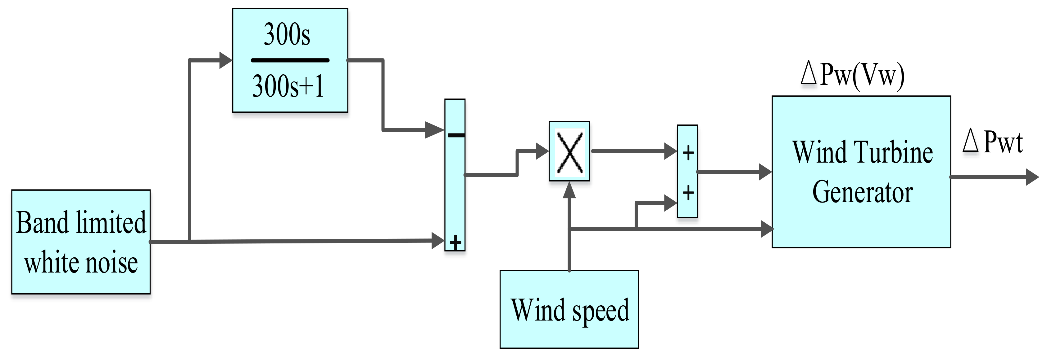
2.2. The Installation of Wind Farm Model

This work presents the high penetration of RESs, including wind power in the investigated hybrid power grid. The professional software MATLAB/SIMULINK program (R2015a) (The MathWorks, Inc., Natick, MA, USA) is used in implementing the simplified model of wind power in order to share its energy in the first area of the studied power grid. The aforementioned wind power model generates power in the same way as the real behavior of the generated power from real wind farms. This is achieved using a white-noise block that is utilized in getting a random speed, which is multiplied by the wind speed, as shown in Figure 3 [47]. The captured output power from the wind model can be formulated in the following equations [47].

$${\mathrm{P}}_{\mathrm{wt}}=\frac{1}{2}{\mathsf{\rho }\mathrm{A}}_{\mathrm{T}}{\mathrm{v}}_{\mathrm{w}}^3{\mathrm{C}}_{\mathrm{p}}\left(\mathsf{\lambda },\mathsf{\beta }\right)$$

(3)

$${\mathrm{C}}_{\mathrm{p}}\left(\mathsf{\lambda },\mathsf{\beta }\right)={\mathrm{C}}_1\left(\frac{{\mathrm{C}}_2}{{\mathsf{\lambda }}_{\mathrm{i}}}-{\mathrm{C}}_3\mathsf{\beta }-{\mathrm{C}}_4{\mathsf{\beta }}^2-{\mathrm{C}}_5\right)\times {\mathrm{e}}^{\frac{-{\mathrm{C}}_6}{{\mathsf{\lambda }}_{\mathrm{i}}}}+{\mathrm{C}}_7{\mathsf{\lambda }}_{\mathrm{T}}$$

(4)

$${\mathsf{\lambda }}_{\mathrm{T}}={ \mathsf{\lambda }}_{\mathrm{T}}^{\mathrm{OP}}=\frac{{\mathsf{\omega }}_{\mathrm{T}}{\mathrm{r}}_{\mathrm{T}}}{{\mathrm{V}}_{\mathrm{W}}}$$

(5)

$$\frac{1}{{\mathsf{\lambda }}_{\mathrm{i}}}=\frac{1}{{\mathsf{\lambda }}_{\mathrm{T}}+0.08\mathsf{\beta }}-\frac{0.035}{{\mathsf{\beta }}^3+1}$$

(6)

All of these mentioned parameter values for the utilized wind farm are presented in [47]. Figure 4 shows the random output power of 257 wind turbine units of 750 KW for each wind power unit. The value of the generated power from the studied wind farm is about 192 MW.

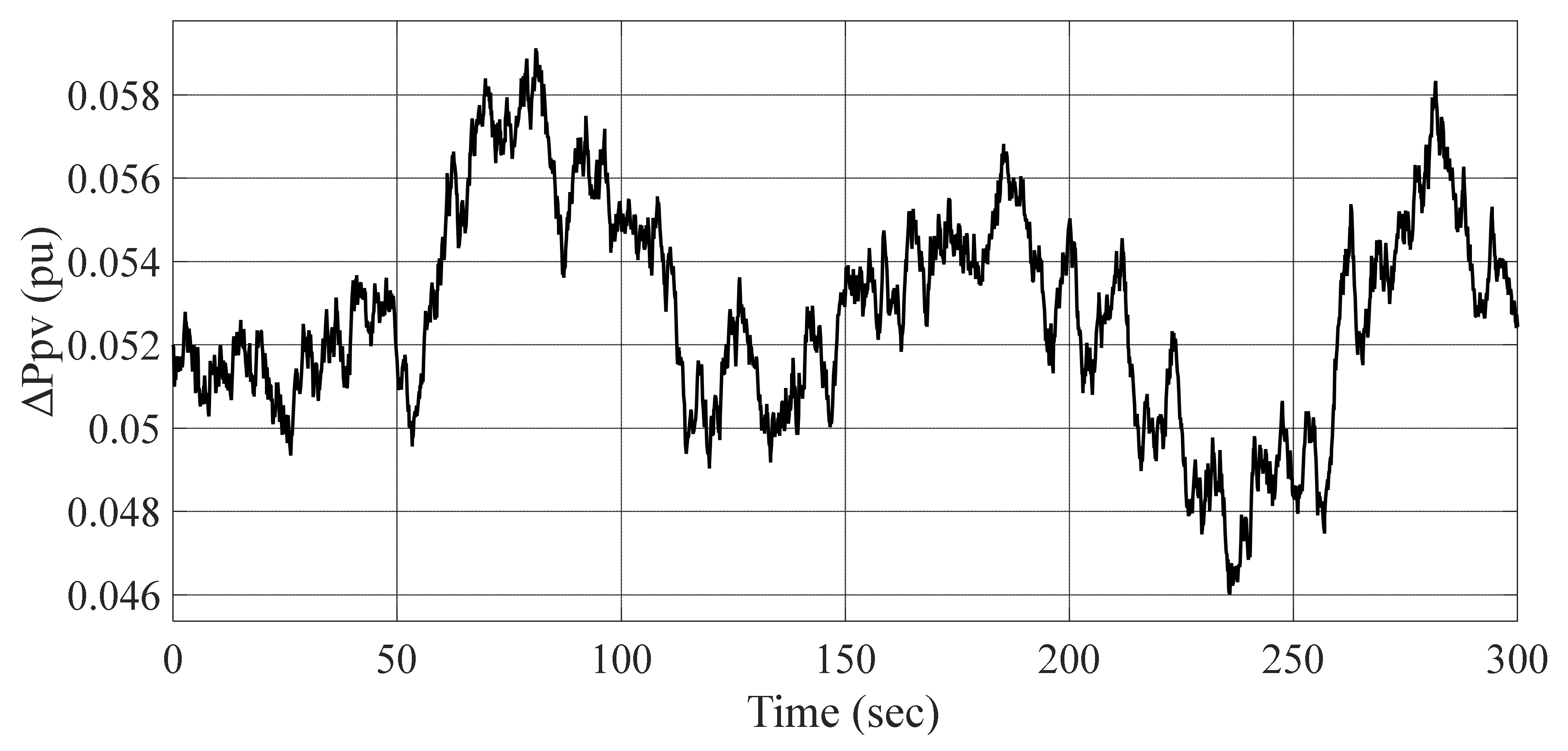
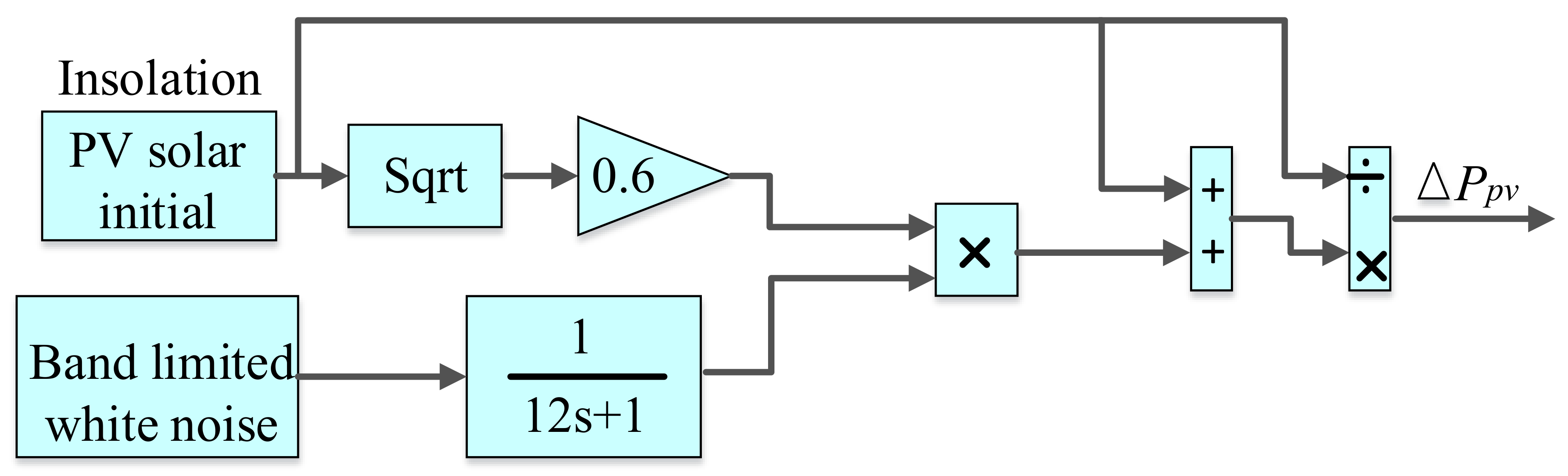
2.3. The Installation of the PV Model

The Photovoltaic (PV) model can be built by utilizing the professional software MATLAB/SIMULINK program (R2015a) described in Figure 5. The generated output power from the model is similar to the real generated output power from a real PV plant. In addition, the output energy of the PV model is penetrated in the second area of the studied power grid at about 116 MW. Here, the white-noise block in the MATLAB program (R2015a) is used for obtaining random output oscillations that are multiplied by the standard output power generated from a real PV plant. The generated energy from the presented PV model can be obtained as formulated in Equation (7) [6]. Figure 6 clarifies the random output power generated from the PV model.

$$\Delta {\mathrm{P}}_{\mathrm{solar} }=0.6\times \sqrt{{\mathrm{P}}_{\mathrm{solar} }}$$

(7)

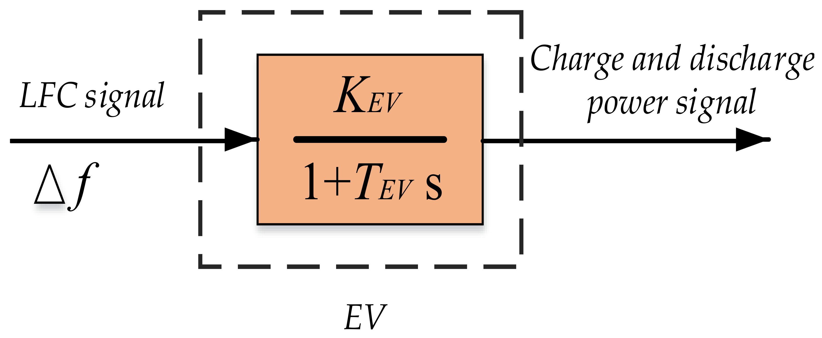
2.4. The Installation of EV Model

EVs can participate in frequency regulation effectively due to the receiving of the LFC order and pass this signal to the EV to control the power during the charging and discharging process. Moreover, the response of the LFC signal can be limited through the availability of the numbers of controllable EVs in the studied power grid and by the state of the charge related to their capacity, whereas the model of the EV is similar to the model of the battery energy storage system, due to the included batteries that supply extra energy to the power grid during fluctuations for regulating the frequency excursions. However, the batteries in EVs may not be in full charging capacity due to the nature of EVs being of mobility and load, which affects the amount of extra energy to tackle the LFC problem. Thus, it is important to check the level of the EV charging to ensure more system enhancement under different system fluctuations. The output power from an EV can be obtained by the first-order transfer function, including the electrical vehicle time constant $T_{EV}$, which equals 0.28 s in series with the electrical vehicle controllers’ gain, $K_{EV}$, which equals 1, where $K_{EV}$ is represented as the ratio of the exchange in charging power of the EV’s batteries to the change of system frequency. The transfer function that represents the EV model is formulated in Equation (8) [49]. Figure 7 describes the EV model that was built in the MATLAB/SIMULINK program (R2015a).

$$\frac{K_{EV} }{1+\mathrm{s} T_{EV}}$$

(8)

3. Control Methodology and Problem Formulation

Due to the high RES penetration, communication time delay, and various types of load perturbations, it is essential to implement a robust controller to enhance the system performance during abnormal conditions. Hence, this study proposes a newly developed controller construction known as a combining TD-TI controller to overcome any fluctuations resulting from the previous considerations/challenges. Moreover, the proposed controller parameters have been selected based on an improved algorithm labeled as QCGO.

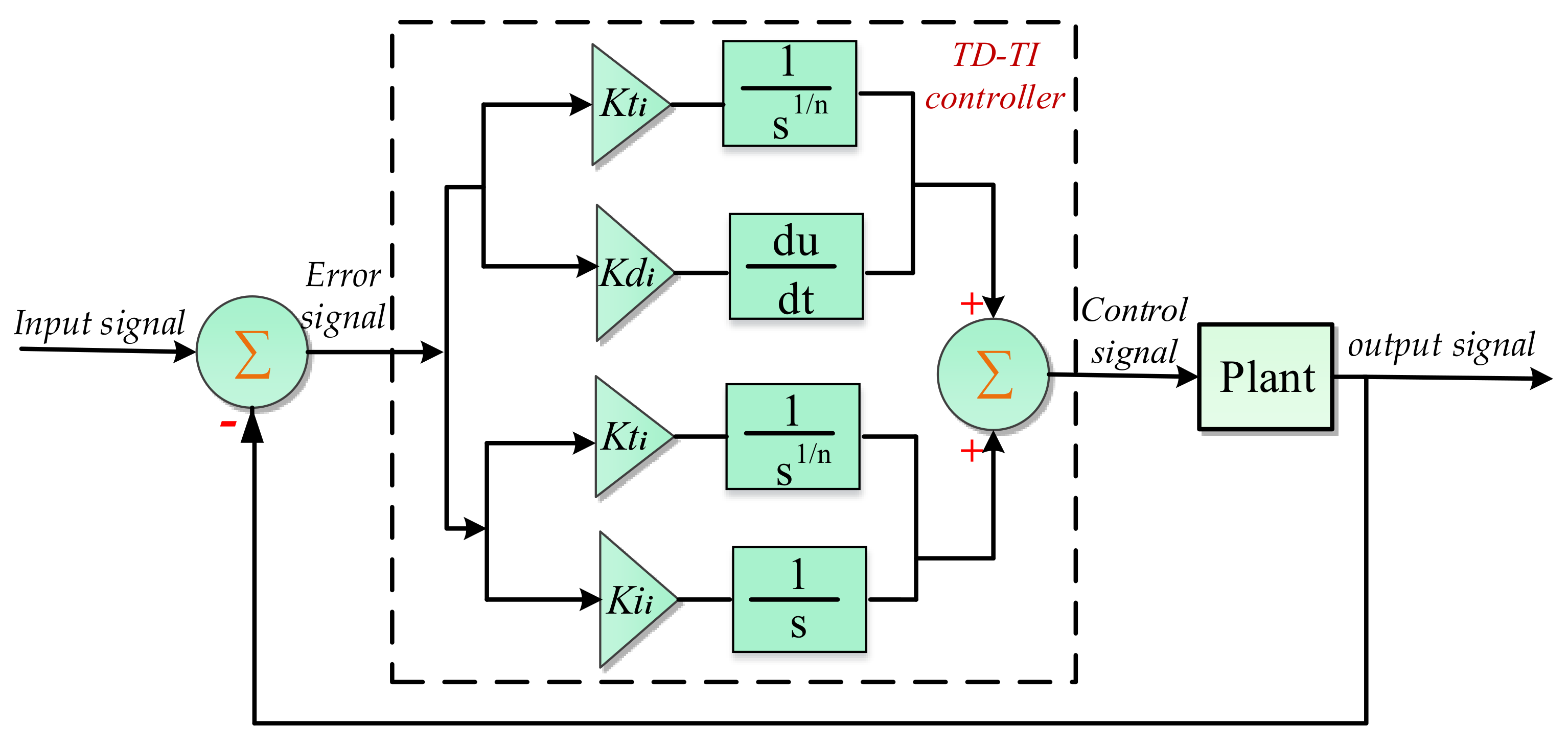
3.1. The Proposed Control Strategy

This paper presents an efficient controller labeled as the combining TD-TI controller, which represents an improved modified structure of the TID controller that is shown in Figure 8. The TID controller is a sort of fractional order controller (FOC) that depends on the fractional-order calculus in its design. The TID controller construction is similar to the PID controller construction except for one difference, which is that the proportional parameter is tilted with a ($1$/${\mathrm{s}}^{\raisebox{1ex}{$1$}\!\left/ \!\raisebox{-1ex}{$\mathrm{n}$}\right.}$) transfer function. In this regard, this paper proposed a combining TD-TI controller, as derived from TID controller, due to the merits of the TID, such as the ability to tune easily, superior fluctuations rejection, and better sensitivity due to variations of the system parametric [50]. The proposed combining TD-TI controller is utilized to enhance the studied power grid performance, such as by damping frequency oscillations in both areas and overcoming fluctuations related to the tie-line power flow. Furthermore, the proposed combining TD-TI controller parameters are selected utilizing an improved QCGO algorithm. In general, the transfer function of the combining TD-TI controller is formulated as follows [50]:

$${\mathrm{G}}_{i1},\mathrm{TD}\left(\mathrm{s}\right)=\frac{K{t}_i}{{\mathrm{S}}^{\frac{1}{\mathrm{n}}}}+K{d}_i\mathrm{S}$$

(9)

$${\mathrm{G}}_{i2},\mathrm{TI}\left(\mathrm{s}\right)=\frac{K{t}_i}{{\mathrm{S}}^{\frac{1}{\mathrm{n}}}}+\frac{K{i}_i}{\mathrm{s}}$$

(10)

$${\mathrm{G}}_i,\mathrm{total}\left(\mathrm{s}\right)={\mathrm{G}}_{i1},\mathrm{TD}\left(\mathrm{s}\right)+{ \mathrm{G}}_{i2},\mathrm{TI}\left(\mathrm{s}\right)$$

(11)

where $i$ refers to the specified proposed controller of the (thermal, hydro, and gas) turbines; thus, ($i$ = 1, 2, 3). The gain values ($K{t}_i$,$K{i}_i,$ and $K{d}_i$) are selected within the range of [0, 10], and $\mathrm{n}$ is tuned in the range of [1, 10]. The control signal of the $i_{th}$ area can be expressed as follows [38]:

$${\mathrm{U}}_i\left(\mathrm{s}\right)={\mathrm{G}}_i,\mathrm{total}\left(\mathrm{s}\right) \times AC{E}_i\left(\mathrm{s}\right)$$

(12)

According to the process of controller designing, there are several sorts of performance criteria, such as the integral time absolute error (ITAE), the integral of squared error (ISE), the integral time squared error (ITSE), and the integral of absolute error (IAE). The criteria of ITAE and ISE are often utilized in the literature for minimizing the objective function due to their merits in comparison to ITSE and IAE, whereas the strategy of the ISE criteria in minimizing the objective function is the integrating of the square of error signal over simulation time. For ease, the ISE criteria can effectively dampen the large errors compared to the small errors as the square of the large errors is larger than the square of the small errors. It can be said that the ISE criteria can penalize the large errors with tolerance for the presence of continuous small errors along with time simulation. Thus, the authors of this work do not hesitate in putting in the ITAE criteria utilized in minimizing the objective function because of the multiplication of the time term by the integral of the absolute error. The multiplied time term in ITAE criteria makes the optimization process more fast which achieves more system stability than utilizing the ISE criteria [51]. The ITAE criteria can be formulated as follows [47]:

$$J=ITAE={{\displaystyle \int }}_0^{Tsim}t. [\left|\Delta f_1\right| + \left|\Delta f_{2 }\right| + \left|\Delta P_{tie }\right|] dt$$

(13)

where $dt$ is represented as the time interval for taking the error signals’ samples over the simulation process.

3.2. The Proposed Optimization Technique

In this subsection, the CGO method is briefly described; then, the process of the QCGO technique is presented.

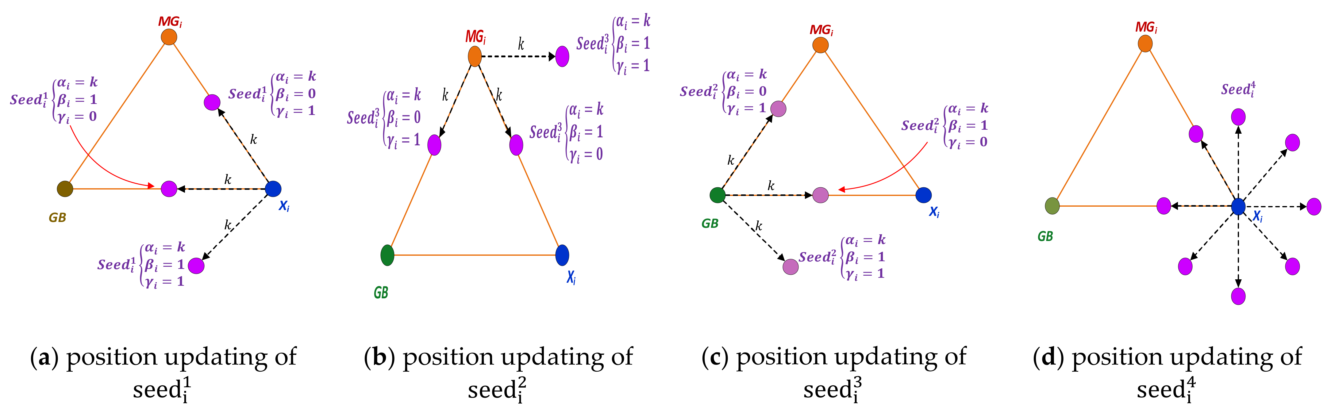
3.2.1. Chaos Game Optimization (CGO) Algorithm

This algorithm is based on certain rules of the chaos theory, where the arrangement of fractals is by the chaos game idea. Firstly, an initialization procedure is configured by determining the initial positions of the solution candidates from the following equations [52]:

$$\mathrm{X}=\left[\begin{array}{c}{\mathrm{X}}_1\\ {\mathrm{X}}_2\\ .\\ .\\ {\mathrm{X}}_{\mathrm{i}}\\ .\\ .\\ {\mathrm{X}}_{\mathrm{n}}\end{array}\right]=\left[\begin{array}{c}{\mathrm{x}}_1^1{ \mathrm{x}}_1^2 \dots ..{ \mathrm{x}}_1^{\mathrm{j}}\dots ..{\mathrm{x}}_1^{\mathrm{d}}\\ {\mathrm{x}}_2^1{ \mathrm{x}}_2^2 \dots ..{ \mathrm{x}}_2^{\mathrm{j}}\dots ..{\mathrm{x}}_2^{\mathrm{d}}\\ \hspace{1em}.\hspace{1em}.\hspace{1em}\hspace{1em}.\hspace{1em}\hspace{1em}.\\ \hspace{1em}.\hspace{1em}.\hspace{1em}\hspace{1em}.\hspace{1em}\hspace{1em}.\\ {\mathrm{x}}_{\mathrm{i}}^1{ \mathrm{x}}_{\mathrm{i}}^2 \dots ..{ \mathrm{x}}_{\mathrm{i}}^{\mathrm{j}}\dots ..{\mathrm{x}}_{\mathrm{i}}^{\mathrm{d}}\\ \hspace{1em}.\hspace{1em}.\hspace{1em}\hspace{1em}.\hspace{1em}\hspace{1em}.\\ \hspace{1em}.\hspace{1em}.\hspace{1em}\hspace{1em}.\hspace{1em}\hspace{1em}.\\ {\mathrm{x}}_{\mathrm{n}}^1{ \mathrm{x}}_{\mathrm{n}}^2 \dots ..{ \mathrm{x}}_{\mathrm{n}}^{\mathrm{j}}\dots ..{\mathrm{x}}_{\mathrm{n}}^{\mathrm{d}}\end{array}\right],\hspace{1em}\hspace{1em}\left\{\begin{array}{c}i=1,2,\dots .,\mathrm{m}\\ j=1,2,\dots ..,\mathrm{d}\end{array}\right.$$

(14)

$${\mathrm{x}}_{\mathrm{i}}^{\mathrm{j}}\left(0\right)={\mathrm{x}}_{\mathrm{i},\min }^{\mathrm{j}}+\mathrm{rand}.\left({\mathrm{x}}_{\mathrm{i},\max }^{\mathrm{j}}-{\mathrm{x}}_{\mathrm{i},\min }^{\mathrm{j}}\right),\hspace{1em}\hspace{1em}\left\{\begin{array}{c}i=1,2,\dots .,\mathrm{m}\\ j=1,2,\dots ..,\mathrm{d}\end{array}\right.$$

(15)

where $\mathrm{d}$ denotes the dimension of the problem and $\mathrm{m}$ refers to the total number of initialized candidates inside the search space. ${\mathrm{x}}_{\mathrm{i},\min }^{\mathrm{j}}$, ${\mathrm{x}}_{\mathrm{i},\max }^{\mathrm{j}}$ are the lower and upper bounds of the decision variables. The position updating process for the temporary triangles is presented in Figure 9. The mathematical representation of the ${\mathrm{seed}}_{\mathrm{i}}^1$, as shown in Figure 9a, is as follows [52]:

$${\mathrm{seed}}_{\mathrm{i}}^1={\mathrm{X}}_{\mathrm{i}}+{\mathsf{\alpha }}_{\mathrm{i}}\times \left({\mathsf{\beta }}_{\mathrm{i}}-\mathrm{GB}-{\mathsf{\gamma }}_{\mathrm{i}}\times {\mathrm{MG}}_{\mathrm{i}}\right),\hspace{1em}\hspace{1em}\mathrm{i}=1,2,\dots .,\mathrm{m}$$

(16)

where $\mathrm{GB}$ is the global best, ${\mathsf{\alpha }}_{\mathrm{i}}$ represents the movement limitation factor, and ${\mathsf{\beta }}_{\mathrm{i}}$ and ${\mathsf{\gamma }}_{\mathrm{i}}$ denote vectors randomly created by numbers in the range of [0, 1]. ${\mathrm{MG}}_{\mathrm{i}}$ is the mean group. From Figure 9b, ${\mathrm{seed}}_{\mathrm{i}}^2$ can be calculated as follows [52]:

$${\mathrm{seed}}_{\mathrm{i}}^2=\mathrm{GB}+{\mathsf{\alpha }}_{\mathrm{i}}\times \left({\mathsf{\beta }}_{\mathrm{i}}\times {\mathrm{X}}_{\mathrm{i}}-{\mathsf{\gamma }}_{\mathrm{i}}\times {\mathrm{MG}}_{\mathrm{i}}\right),\hspace{1em}\hspace{1em}\mathrm{i}=1,2,\dots .,\mathrm{m}$$

(17)

While ${\mathrm{seed}}_{\mathrm{i}}^3$, which is displayed in Figure 9c, is mathematically computed as below [52]:

$${\mathrm{seed}}_{\mathrm{i}}^3={\mathrm{MG}}_{\mathrm{i}}+{\mathsf{\alpha }}_{\mathrm{i}}\times \left({\mathsf{\beta }}_{\mathrm{i}}\times {\mathrm{X}}_{\mathrm{i}}-{\mathsf{\gamma }}_{\mathrm{i}}\times \mathrm{GB}\right),\hspace{1em}\hspace{1em}\mathrm{i}=1,2,\dots .,\mathrm{m}$$

(18)

Finally, ${\mathrm{seed}}_{\mathrm{i}}^4$, which is shown in Figure 9d, can be mathematically represented as follows [52]:

$${\mathrm{seed}}_{\mathrm{i}}^4={\mathrm{X}}_{\mathrm{i}}\left({\mathrm{x}}_{\mathrm{i}}^{\mathrm{k}}={\mathrm{x}}_{\mathrm{i}}^{\mathrm{k}}+\mathrm{R}\right),\hspace{1em} \mathrm{k}=\left[1,2,\dots .,\mathrm{d}\right]$$

(19)

where $\mathrm{R}$ refers to a vector with random numbers in the range of [0, 1].

3.2.2. The Proposed Quantum Chaos Game Optimization (QCGO) Algorithm

In this subsection, quantum mechanics is used to develop the original CGO algorithm. This quantum model of a CGO algorithm is called here QCGO algorithm. Quantum mechanics was employed to develop the PSO in [54]. In the quantum model, by employing the Monte Carlo method, the solution ${\mathrm{x}}_{\mathrm{new}4}$ is calculated from this equation [54]:

If h ≥ 0.5

$${\mathrm{x}}_{\mathrm{new}1}=\mathrm{p}+\mathsf{\alpha }·\left|{\mathrm{Mbest}}_{\mathrm{i}}-{\mathrm{X}}_{\mathrm{i}}\right| ·\ln \left(1/\mathrm{u}\right)$$

(20)

Else

$${\mathrm{x}}_{\mathrm{new}1}=\mathrm{p}-\mathsf{\alpha }·\left|{\mathrm{Mbest}}_{\mathrm{i}}-{\mathrm{X}}_{\mathrm{i}}\right| ·\ln \left(1/\mathrm{u}\right)$$

(21)

End.

where $\mathsf{\alpha }$ refers to a design parameter, $\mathrm{u}$ and h denote uniform probability distribution in the range [0, 1], and Mbest is the mean best of the population and is defined as the mean of the $\mathrm{GB}$ positions. It can be calculated as follows [54]:

$$\mathrm{Mbest}=\frac{1}{\mathrm{N}}{\displaystyle \sum }_{\mathrm{l}=1}^{\mathrm{N}}{\mathrm{p}}_{\mathrm{g},\mathrm{l}}\left(\mathrm{i}\right)$$

(22)

where g is the index of the best solution among all the solutions.

4. The Procedure of the Improved QCGO Algorithm

The Performance of QCGO

The proposed QCGO algorithm competency and performance are evaluated on the numerous benchmark functions, using the statistical measurements, such as best values, mean values, median values, worst values, and standard deviation (STD), for the best solutions achieved using the proposed technique and the other well-known algorithms. The results attained by the QCGO technique are compared with three recent meta-heuristic techniques, including SDO [55], WOA [56], and BOA [57], in addition to the conventional CGO. All of the mentioned techniques were executed for the maximum number of iterations of the function of 200 and a population size of 50 for 20 independent runs, using Matlab R2016a working on Windows 8.1, 64 bit (Microsoft, Albuquerque, NM, USA). All computations were performed on a Core i5-4210U CPU@ 2.40 GHz of speed (Intel Corporation, Santa Clara, CA, USA) and 8 GB of RAM. Figure 10 shows the qualitative metrics on F1, F2, F3, F5, F6, F8, F10, F12, F15, F18, and F22, with 2D views of the functions, convergence curve, average fitness history, and search history.

Table 4. Results of unimodal benchmark functions.

Function		QCGO	CGO	SDO	WOA	BOA
F1	Best	2.4$\times {10}^{-126}$	1.52 $\times {10}^{-58}$	1.39 $\times {10}^{-55}$	1.92 $\times {10}^{-40}$	3.87 $\times {10}^{-08}$
	Mean	1.4$\times {10}^{-122}$	4.97 $\times {10}^{-55}$	1.37 $\times {10}^{-51}$	7.2 $\times {10}^{-34}$	4.96 $\times {10}^{-08}$
	Median	4.8$\times {10}^{-124}$	3.86 $\times {10}^{-56}$	3.74 $\times {10}^{-54}$	2.28 $\times {10}^{-35}$	4.95 $\times {10}^{-08}$
	Worst	1.2$\times {10}^{-121}$	3.9 $\times {10}^{-54}$	8.43 $\times {10}^{-51}$	4.34 $\times {10}^{-33}$	6 $\times {10}^{-08}$
	Std	3.7$\times {10}^{-122}$	9.85 $\times {10}^{-55}$	2.74 $\times {10}^{-51}$	1.34 $\times {10}^{-33}$	4.94 $\times {10}^{-09}$
F2	Best	4.2$\times {10}^{-65}$	3.64 $\times {10}^{-31}$	1.83 $\times {10}^{-29}$	4.41 $\times {10}^{-24}$	4.26 $\times {10}^{-06}$
	Mean	1.85$\times {10}^{-63}$	9.17 $\times {10}^{-29}$	3.76 $\times {10}^{-25}$	5.82 $\times {10}^{-21}$	5.71 $\times {10}^{-06}$
	Median	6.63$\times {10}^{-64}$	1.96 $\times {10}^{-29}$	1.13 $\times {10}^{-26}$	1.34 $\times {10}^{-21}$	5.77 $\times {10}^{-06}$
	Worst	7.99$\times {10}^{-63}$	9.73 $\times {10}^{-28}$	3.98 $\times {10}^{-24}$	5.99 $\times {10}^{-20}$	7.58 $\times {10}^{-06}$
	Std	2.41$\times {10}^{-63}$	2.23 $\times {10}^{-28}$	9.1 $\times {10}^{-25}$	1.34 $\times {10}^{-20}$	9.92 $\times {10}^{-07}$
F3	Best	2.68 $\times {10}^{-42}$	2.41 $\times {10}^{-40}$	6.27$\times {10}^{-46}$	0.027608	3.85 $\times {10}^{-08}$
	Mean	1.66 $\times {10}^{-36}$	6.69$\times {10}^{-37}$	6.91 $\times {10}^{-34}$	1.518335	4.67 $\times {10}^{-08}$
	Median	4.45 $\times {10}^{-39}$	1.39 $\times {10}^{-38}$	1.4$\times {10}^{-39}$	1.011391	4.61 $\times {10}^{-08}$
	Worst	1.82 $\times {10}^{-35}$	7.13$\times {10}^{-36}$	1.38 $\times {10}^{-32}$	3.914695	5.57 $\times {10}^{-08}$
	Std	4.41 $\times {10}^{-36}$	1.68$\times {10}^{-36}$	3.09 $\times {10}^{-33}$	1.18435	5.02 $\times {10}^{-09}$
F4	Best	5.12$\times {10}^{-53}$	3.76 $\times {10}^{-37}$	1.11 $\times {10}^{-26}$	0.99528	8.45 $\times {10}^{-06}$
	Mean	6.71$\times {10}^{-51}$	3.7 $\times {10}^{-23}$	4.52 $\times {10}^{-23}$	53.18395	1.02 $\times {10}^{-05}$
	Median	2.13$\times {10}^{-51}$	1.4 $\times {10}^{-23}$	1.14 $\times {10}^{-23}$	60.93168	1.02 $\times {10}^{-05}$
	Worst	3.32$\times {10}^{-50}$	1.81 $\times {10}^{-22}$	1.94 $\times {10}^{-22}$	89.09969	1.15 $\times {10}^{-05}$
	Std	9.43$\times {10}^{-51}$	5.38 $\times {10}^{-23}$	6.34 $\times {10}^{-23}$	29.69543	8.51 $\times {10}^{-07}$
F5	Best	18.11582	17.11845	27.90967	27.88483	28.89058
	Mean	19.57861	19.61026	28.65096	28.27419	28.92369
	Median	19.35622	19.29265	28.74726	28.43647	28.91978
	Worst	22.2175	21.59463	28.98699	28.7227	28.96927
	Std	1.149609	1.224882	0.295026	0.28925	0.021273
F6	Best	1.75$\times {10}^{-14}$	6.75 $\times {10}^{-14}$	0.039957	0.303542	4.311051
	Mean	2.86$\times {10}^{-12}$	2.63 $\times {10}^{-12}$	2.568541	0.655907	5.211726
	Median	7.7$\times {10}^{-14}$	6.23 $\times {10}^{-13}$	2.038779	0.62203	5.06303
	Worst	4.89 $\times {10}^{-11}$	2.57$\times {10}^{-11}$	7.250251	1.16408	6.168001
	Std	1.09 $\times {10}^{-11}$	6.11$\times {10}^{-12}$	1.852701	0.210811	0.509499
F7	Best	1.02$\times {10}^{-05}$	0.000197	8.66 $\times {10}^{-05}$	0.0004	0.000983
	Mean	0.000263	0.00092	0.002356	0.00542	0.002696
	Median	0.000231	0.00085	0.001136	0.003763	0.002776
	Worst	0.000768	0.001975	0.013813	0.019069	0.005116
	Std	0.000177	0.000583	0.003331	0.005011	0.001104

The best values obtained are in bold.

,

Table 5. Results of multimodal benchmark functions.

Function		QCGO	CGO	SDO	WOA	BOA
F8	Best	−1671.01	−1770.26	−1655	−1909.05	−921.028
	Mean	−1465.24	−1490.19	−1312.83	−1786.9	−766.513
	Median	−1453.48	−1483.32	−1385.86	−1907.06	−778.594
	Worst	−1313.6	−1235.22	−598.802	−1632.06	−647.792
	Std	108.2831	123.7418	294.008	138.0759	61.76107
F9	Best	0.00	0.00	4.33 $\times {10}^{-30}$	0.00	5.17 $\times {10}^{-09}$
	Mean	0.00	0.00	1.75 $\times {10}^{-22}$	1.14 $\times {10}^{-14}$	0.003376
	Median	0.00	0.00	4.17 $\times {10}^{-25}$	0.00	3.86 $\times {10}^{-06}$
	Worst	0.00	0.00	3.02 $\times {10}^{-21}$	1.14 $\times {10}^{-13}$	0.047754
	Std	0.00	0.00	6.75 $\times {10}^{-22}$	2.97 $\times {10}^{-14}$	0.010836
F10	Best	8.88$\times {10}^{-16}$	8.88$\times {10}^{-16}$	8.88$\times {10}^{-16}$	4.44 $\times {10}^{-15}$	1.67 $\times {10}^{-05}$
	Mean	2.49 $\times {10}^{-15}$	3.2 $\times {10}^{-15}$	8.88$\times {10}^{-16}$	1.33 $\times {10}^{-14}$	4.77 $\times {10}^{-05}$
	Median	8.88$\times {10}^{-16}$	4.44 $\times {10}^{-15}$	8.88$\times {10}^{-16}$	1.15 $\times {10}^{-14}$	4.55 $\times {10}^{-05}$
	Worst	4.44 $\times {10}^{-15}$	4.44 $\times {10}^{-15}$	8.88$\times {10}^{-16}$	3.29 $\times {10}^{-14}$	7.94 $\times {10}^{-05}$
	Std	1.81 $\times {10}^{-15}$	1.74 $\times {10}^{-15}$	0.00	8.11 $\times {10}^{-15}$	1.69 $\times {10}^{-05}$
F11	Best	0.00	0.00	0.00	0.00	3.23 $\times {10}^{-08}$
	Mean	0.00	0.00	0.00	0.021832	4.29 $\times {10}^{-08}$
	Median	0.00	0.00	0.00	0.00	4.22 $\times {10}^{-08}$
	Worst	0.00	0.00	0.00	0.26626	5.81 $\times {10}^{-08}$
	Std	0.00	0.00	0.00	0.068973	6.29 $\times {10}^{-09}$
F12	Best	3.66$\times {10}^{-16}$	1.34 $\times {10}^{-15}$	0.001152	0.006052	0.33315
	Mean	5.69$\times {10}^{-15}$	8.04 $\times {10}^{-14}$	0.23467	0.022239	0.565424
	Median	2.26$\times {10}^{-15}$	1.93 $\times {10}^{-14}$	0.067805	0.015529	0.562862
	Worst	3.32$\times {10}^{-14}$	5.01 $\times {10}^{-13}$	1.492821	0.087947	0.754521
	Std	8.06$\times {10}^{-15}$	1.36 $\times {10}^{-13}$	0.352063	0.018774	0.108748
F13	Best	6.36$\times {10}^{-14}$	7.4 $\times {10}^{-13}$	0.046216	0.400281	2.497296
	Mean	0.007142	0.036733	1.867552	0.687522	2.894224
	Median	0.005494	0.010987	1.934246	0.598054	2.982946
	Worst	0.043949	0.233414	2.999924	1.321352	3.109356
	Std	0.010254	0.065978	0.961284	0.248523	0.153028

The best values obtained are in bold.

and

Table 6. Results of composite benchmark functions.

Function		QCGO	CGO	SDO	WOA	BOA
F14	Best	0.998004	0.998004	0.998004	0.998004	0.998004
	Mean	0.998004	0.998004	3.494696	2.230204	1.301281
	Median	0.998004	0.998004	1.495017	1.495017	1.024436
	Worst	0.998004	0.998004	12.67051	10.76318	2.983027
	Std	0.00	5.09 $\times {10}^{-17}$	3.953203	2.241367	0.534994
F15	Best	0.000307	0.000307	0.000307	0.000311	0.000315
	Mean	0.000307	0.000353	0.00067	0.000626	0.000487
	Median	0.000307	0.000307	0.000527	0.000578	0.000405
	Worst	0.000307	0.001223	0.002121	0.001528	0.000917
	Std	1.68$\times {10}^{-19}$	0.000205	0.000473	0.000342	0.000173
F16	Best	−1.03163	−1.03163	−1.03163	−1.03163	−1.40747
	Mean	−1.03163	−1.03163	−1.03005	−1.03163	−1.18199
	Median	−1.03163	−1.03163	−1.03163	−1.03163	−1.18517
	Worst	−1.03163	−1.03163	−1.00046	−1.03163	−1.07213
	Std	2.22$\times {10}^{-16}$	2.28 $\times {10}^{-16}$	0.006966	1.94 $\times {10}^{-08}$	0.088213
F17	Best	0.397887	0.397887	0.397887	0.397887	0.398293
	Mean	0.397887	0.397887	0.397987	0.397896	0.409332
	Median	0.397887	0.397887	0.397887	0.39789	0.406611
	Worst	0.397887	0.397887	0.399795	0.397967	0.461881
	Std	0.00	0.00	0.000426	1.78 $\times {10}^{-05}$	0.014049
F18	Best	3.00	3.00	3.00	3.000001	3.000586
	Mean	3.00	3.00	3.001185	3.000069	3.092676
	Median	3.00	3.00	3.00	3.000026	3.054728
	Worst	3.00	3.00	3.023537	3.000668	3.425476
	Std	2.7$\times {10}^{-16}$	6.03 $\times {10}^{-16}$	0.005261	0.000147	0.108993
F19	Best	−0.30048	−0.30048	−0.30048	−0.30048	−0.30048
	Mean	−0.30048	−0.30048	−0.2893	−0.30048	−0.30048
	Median	−0.30048	−0.30048	−0.30038	−0.30048	−0.30048
	Worst	−0.30048	−0.30048	−0.19165	−0.30048	−0.30048
	Std	1.14$\times {10}^{-16}$	1.14$\times {10}^{-16}$	0.026531	1.14$\times {10}^{-16}$	3.74 $\times {10}^{-06}$
F20	Best	−3.322	−3.322	−3.322	−3.31923	$-3.3\times {10}^{-05}$
	Mean	−3.26849	−3.28038	−3.09697	−2.98949	$-1.6\times {10}^{-06}$
	Median	−3.322	−3.322	−3.2031	−3.15019	$-1.5\times {10}^{-40}$
	Worst	−3.2031	−3.2031	−0.89904	−1.57922	$-2\times {10}^{-134}$
	Std	0.060685	0.058182	0.550986	0.479795	7.35$\times {10}^{-06}$
F21	Best	−10.1532	−10.1532	−10.1532	−10.1528	−4.61081
	Mean	−10.1532	−9.90058	−8.703	−7.35262	−4.0759
	Median	−10.1532	−10.1532	−10.1532	−10.0113	−4.12522
	Worst	−10.1532	−5.10077	−4.99677	−2.59723	−3.18003
	Std	3.21$\times {10}^{-15}$	1.129757	2.23952	3.245445	0.379957
F22	Best	−10.4029	−10.4029	−10.4029	−10.4008	−4.76031
	Mean	−10.4029	−10.4029	−8.45822	−7.90953	−3.74931
	Median	−10.4029	−10.4029	−10.4029	−10.2376	−3.64889
	Worst	−10.4029	−10.4029	−1.0677	−3.69711	−2.93305
	Std	3.05$\times {10}^{-15}$	3.36 $\times {10}^{-15}$	3.128689	2.779744	0.479377
F23	Best	−10.5364	−10.5364	−10.5364	−10.5297	−4.51577
	Mean	−9.99562	−9.93332	−7.90449	−7.3919	−3.38426
	Median	−10.5364	−10.5364	−10.5357	−7.79854	−3.60414
	Worst	−5.12848	−3.83543	−3.79083	−1.67334	−1.95854
	Std	1.664525	1.868952	3.015319	3.33909	0.720921

The best values obtained are in bold.

show the statistical results of the proposed QCGO technique and other algorithms when applied for the three types of benchmark functions (unimodal, multimodal, and composite, respectively). The best-obtained values using the QCGO, CGO, SDO, WOA, and BOA algorithms are displayed in bold. It is clearly seen that the QCGO algorithm achieves the optimal solution for most of those benchmark functions. The convergence curves of these techniques for those functions are illustrated in Figure 11, and the boxplots for each algorithm for these functions are displayed in Figure 12. From those figures, it is seen that the QCGO technique reached a stable point for all functions, and the boxplots of the proposed QCGO technique are very narrow and stable for most functions compared to the other techniques.

5. Simulation Results and Discussions

In this study, the proposed control strategy is implemented in the secondary control loop with the high integration of RESs, considering different load variation types to restore the studied system frequency at the pre-defined value, where the presented control strategy relied on the combining TD-TI controller, which is optimally designed by an improved QCGO algorithm to obtain the minimum value of the frequency fluctuations for the studied power grid. Moreover, the performance of the suggested control strategy is compared with other control strategies (i.e., TID and PID). All of the simulation results for the studied two-area, multi-unit power grid are implemented using the professional software MATLAB/SIMULINK^® program (R2015a) to ensure the efficacy of the proposed controller in enhancing the studied system performance. The code of the proposed QCGO algorithm is an m-file linked to the studied model for the optimization process. The simulation results are performed on a PC with Intel Core i5-2.60 GHz with 4.00 GB of RAM. The frequency stability has been assessed by applying different operating conditions through the following scenarios.

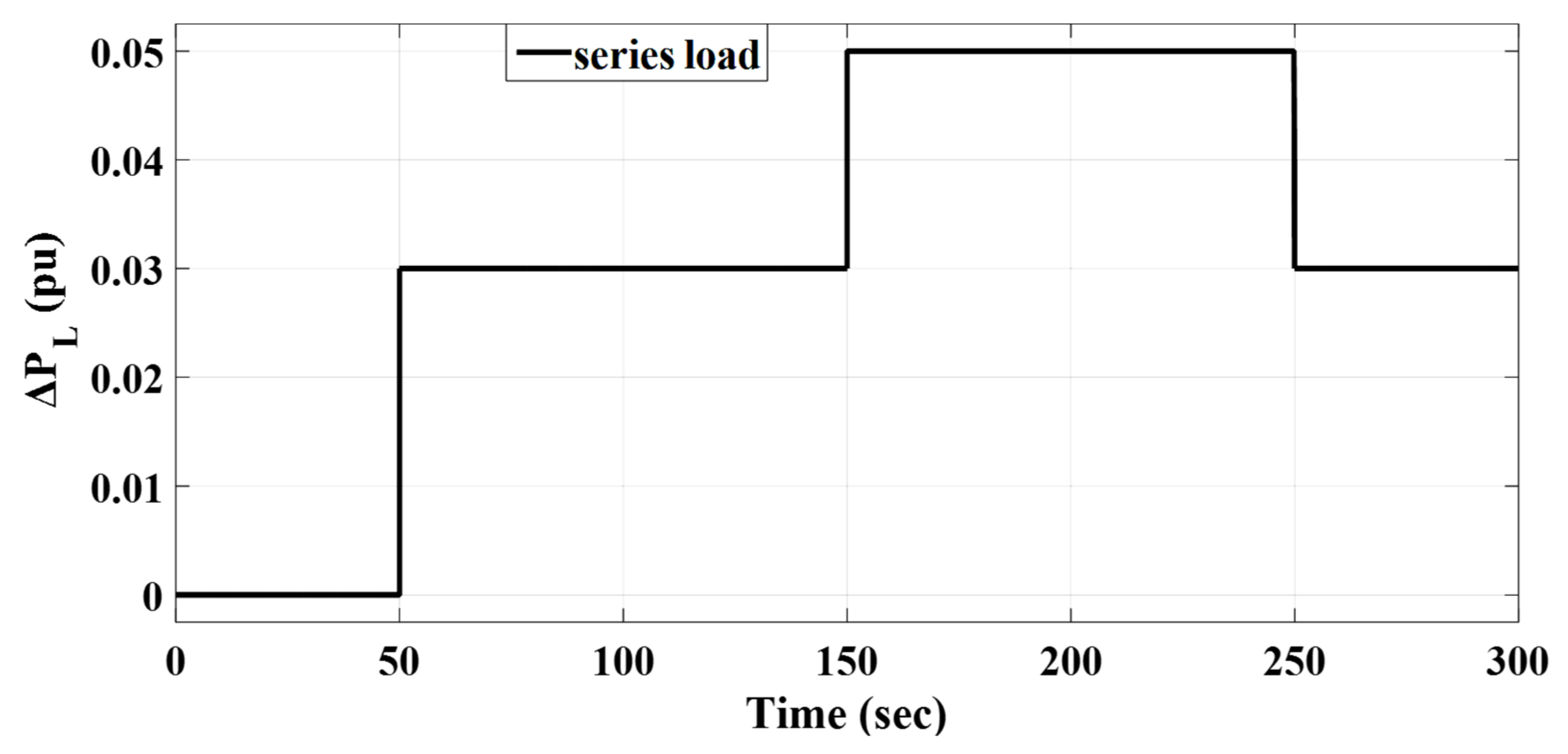
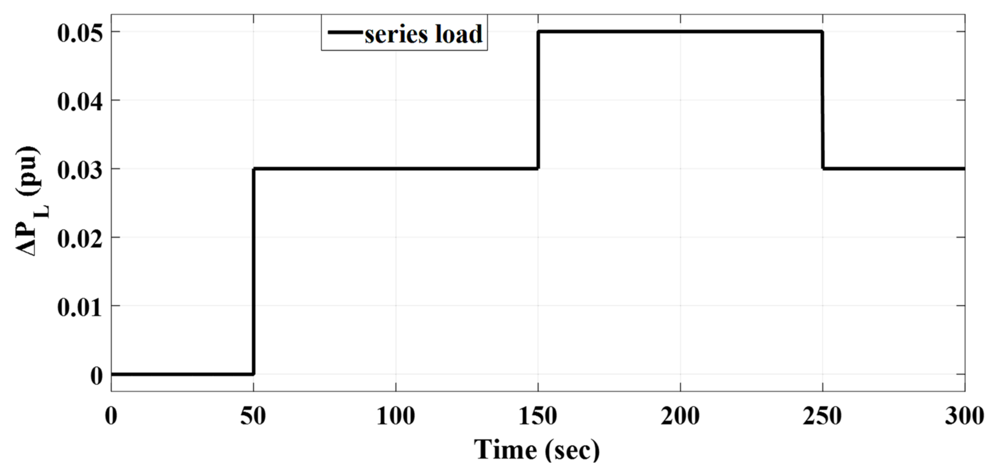
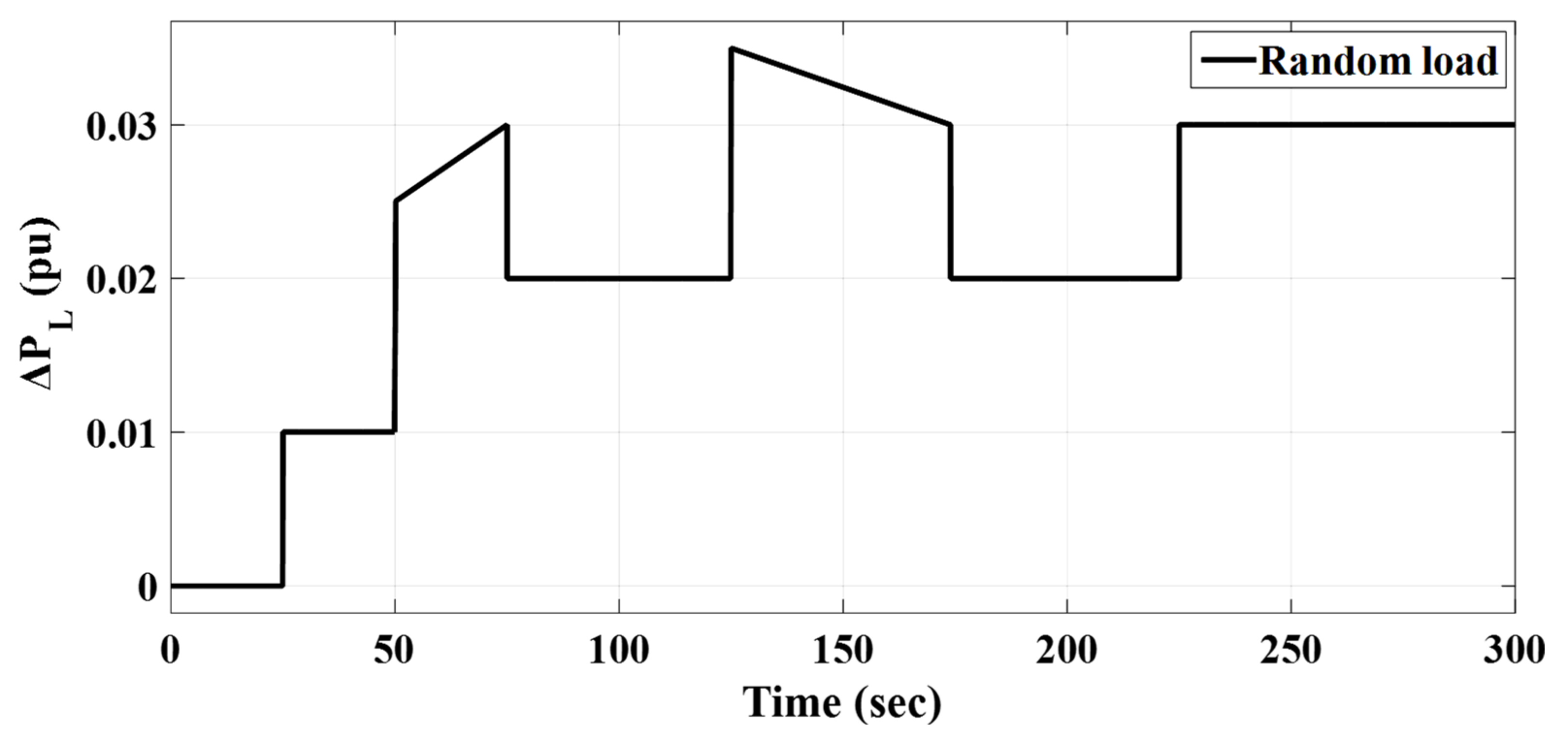
• Scenario A: evaluation of the studied power grid performance considering various load variation types (i.e., SLP, series SLP, and RLV).
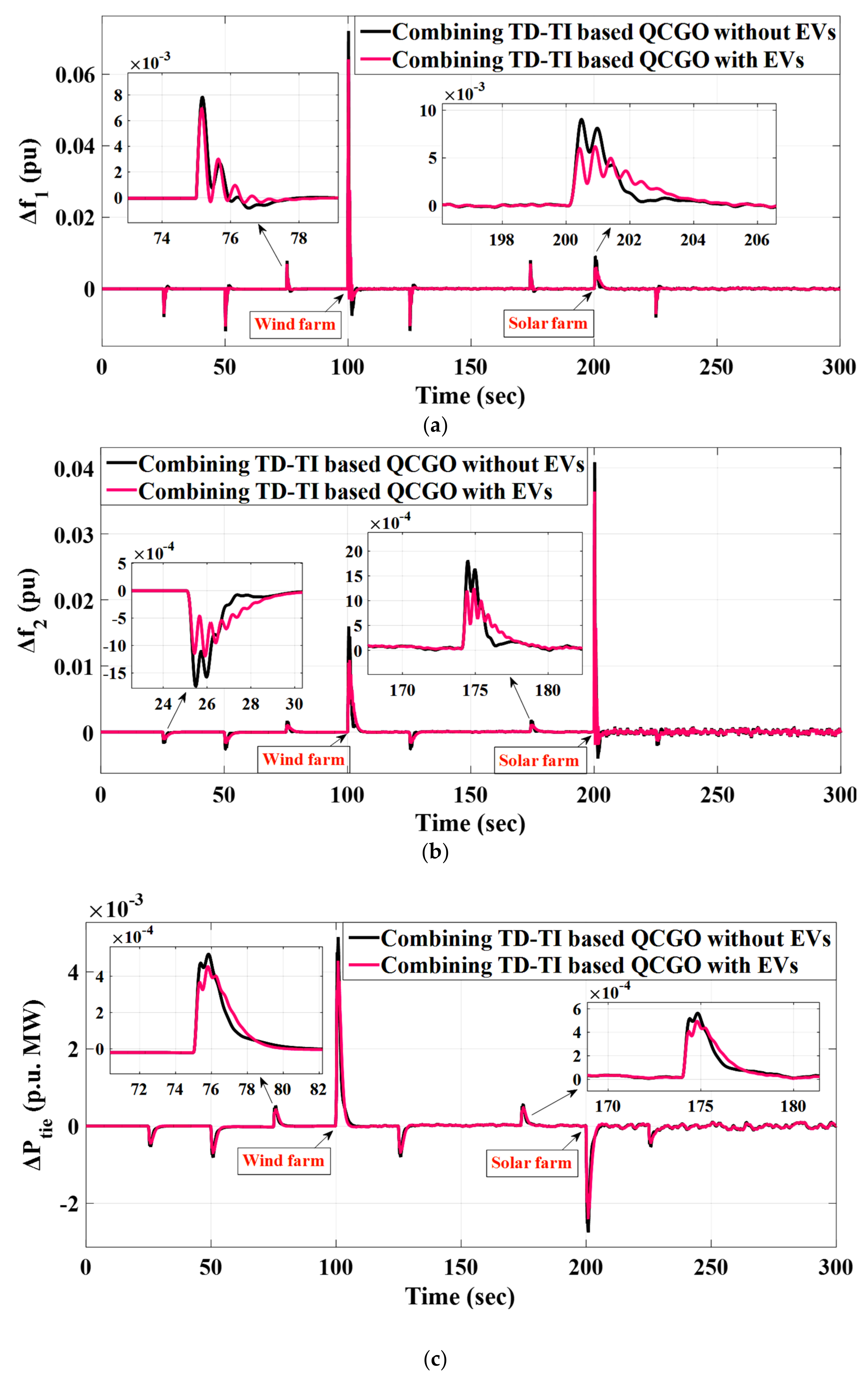
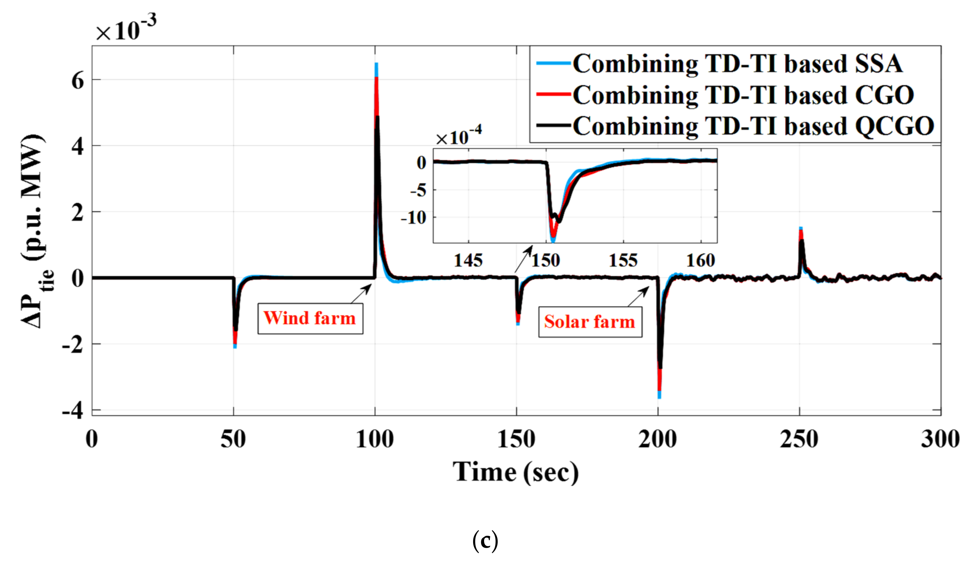
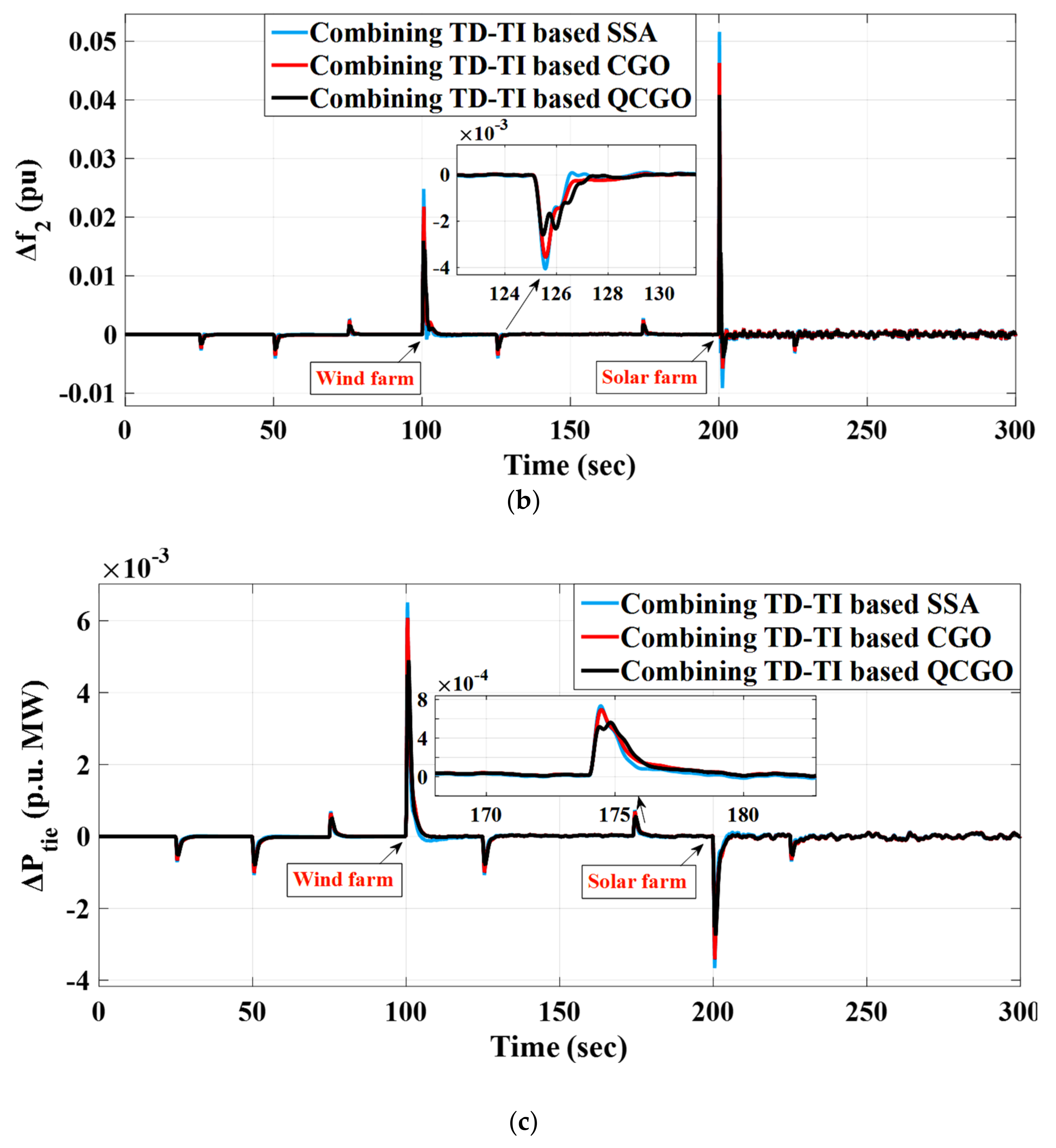
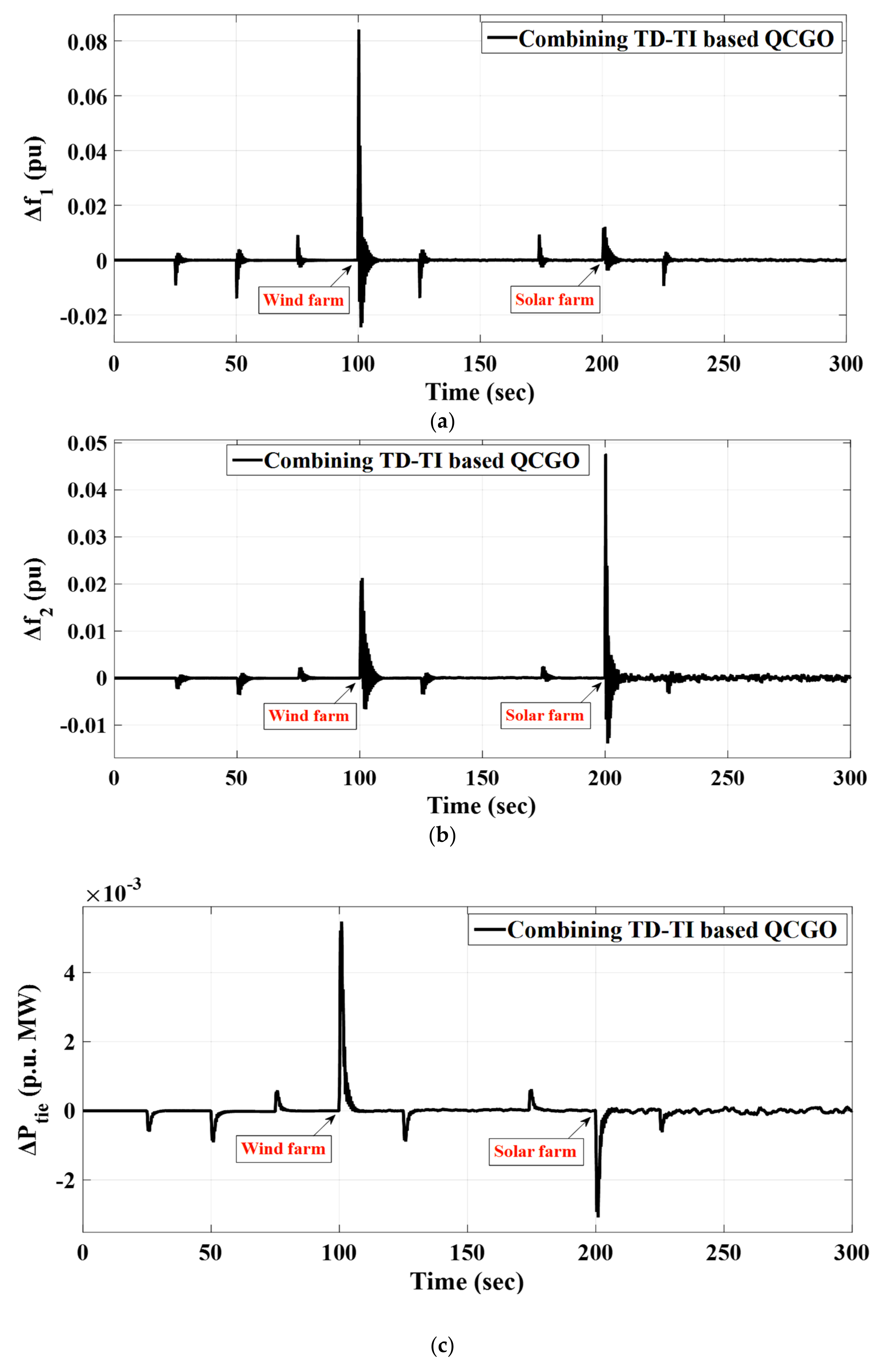
• Scenario B: evaluation of the studied power grid performance considering high penetration of RESs in both areas with series SLP and RLV.
• Scenario C: evaluation of the studied power grid performance considering communication time delay.
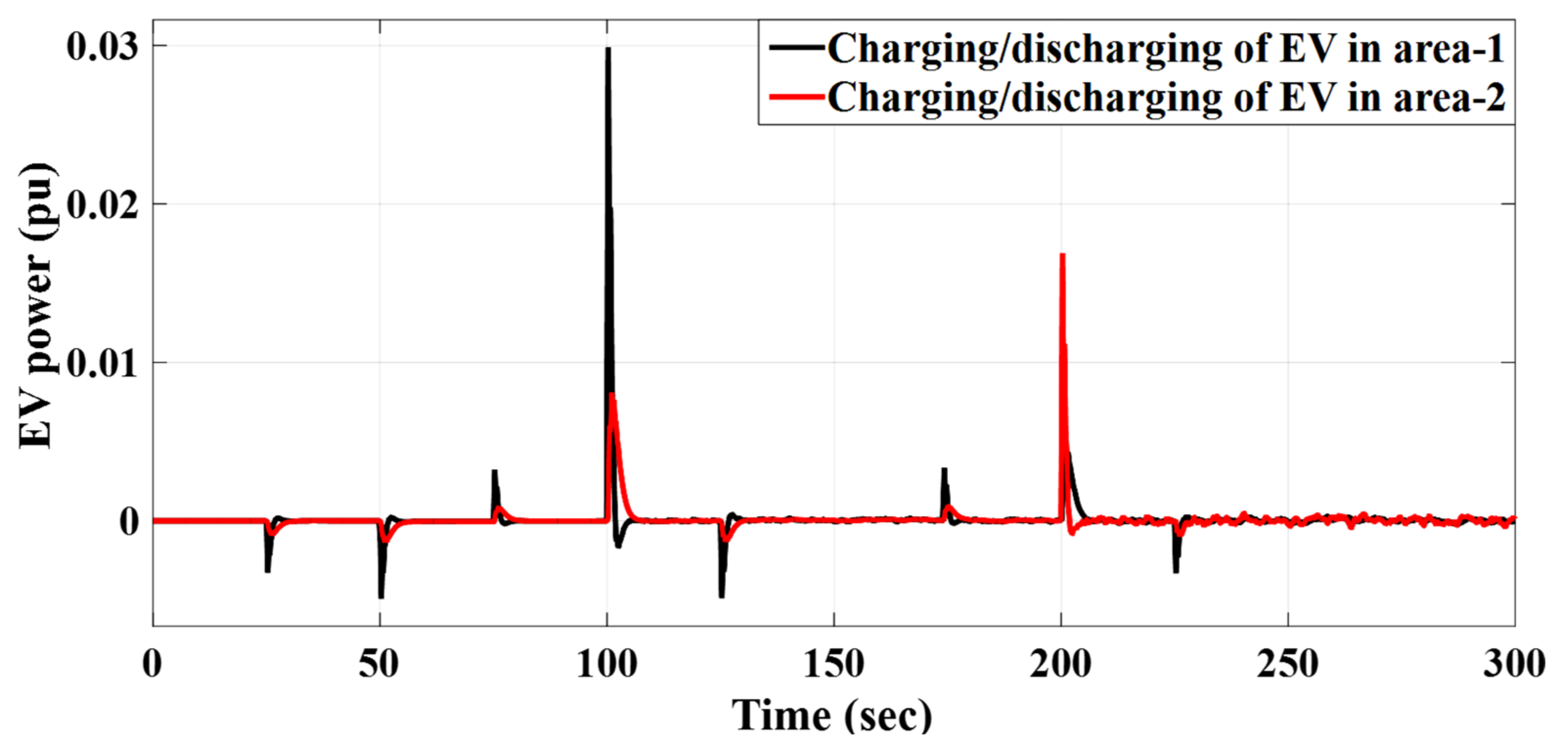
• Scenario D: evaluation of the studied power grid performance considering EV integration in both areas.

The studied power grid performance can be evaluated by measuring the value of the best objective function that is represented by the ITAE value over the iterations. For most, several initial considerations must be addressed while optimizing the proposed TD-TI controller using the proposed improved QCGO algorithm, such as the search agent number that equals 30 and the total iterations/attempts that equal 100. The convergence curve that is shown in Figure 13 clarifies the performance of the proposed combining TD-TI controller based on QCGO compared to the combining TD-TI controller based on CGO and SSA and compared with the TID controller based on QCGO and CGO. The demonstrated convergence curve can be obtained considering a 1% SLP at 10 s in the first area of the studied power grid, without any RESs penetration in both areas. It is clear that the proposed combining TD-TI controller based on QCGO attained the lowest value of the objective function compared to the other mentioned controllers that relied on various optimization techniques. As a result, the convergence curve elucidates the effectiveness of the proposed QCGO algorithm. It can be seen that the curve behavior of the proposed TD-TI based on QCGO starts with a 0.1098 objective function value; then, this value drops along the iterations to end up at the final iteration with a 0.0729 objective function value, whereas the behavior of the proposed controller/proposed algorithm can be described as it reaches the best objective function value quickly compared to the other utilized controllers via different techniques. Moreover, it can be said, the rest curve behaviors are far from the optimum goal achieved by the suggested controller using QCGO, demonstrating its robustness in damping the oscillations effectively.

Scenario A: evaluation of the studied system performance considering different load variation types (i.e., SLP, series SLP, and random load).

This scenario included a fair-maiden comparison between the proposed combining TD-TI controller utilizing the QCGO algorithm and the other published controllers, such as the PID controller based on TLBO and AOA. Moreover, the proposed combining TD-TI controller based on the improved QCGO technique was compared with different mentioned controllers, such as the TID controller based on QCGO and CGO and the combining TD-TI controller based on CGO and SSA, to test the stability of the studied power grid performance.

Case A.1: The SLP was selected as a challenge by applying it in the first area of the studied power grid to test the efficacy of the proposed combining TD-TI controller in enhancing the system performance. The applicable SLP occurred at 10 s with a 1% value, whereas the SLP can occur in the electrical power grids through disconnecting some generators from all the generation stations that may lead to blackouts with the shutdown of all the stations’ generators. In addition, SLP may be represented as an unexpected switch of the connected electrical loads that may lead to instability in the system performance by increasing the wear and tear on the generators in the power grid.

Case A.1.1: This case presents a comparison between the performance of the proposed combining TD-TI controller in this work and the other published performances of the PID controller, to prove the efficacy of the proposed controller in attaining the main target (damping frequency oscillations).

Table 7. The optimum parameters of the different controllers.

Controller Properties	Thermal	Hydro	Gas
Combining TD-TI-based QCGO	$k_{t1}=9.9999, k_{d1}=9.9988, n_1$ = 3.5626 $k_{t2}=9.9991, k_{i2}=5.4425, n_2$ = 3.5311	$k_{t1}=9.9834, k_{d1}=3.8871, n_1$ = 9.9468 $k_{t2}=9.5835, k_{i2}=1.0016, n_2$ = 9.9508	$k_{t1}=9.998, k_{d1}=9.9973, n_1$ = 3.7621 $k_{t2}=9.9951, k_{i2}=9.9704, n_2$ = 1.2938
Combining TD-TI-based CGO	$k_{t1}=9.9998, k_{d1}=6.9628, n_1$ = 3.5715 $k_{t2}=9.9977, k_{i2}=5.033 n_2$ = 3.4737	$k_{t1}=9.98, k_{d1}=2.7245, n_1$ = 9.9129 $k_{t2}=7.2945, k_{i2}=1.052 n_2$ = 9.9827	$k_{t1}=9.9998, k_{d1}=8.4098, n_1$ = 1.2782 $k_{t2}=9.9966, k_{i2}=9.9989 n_2$ = 6.9549
Combining TD-TI-based SSA	$k_{t1}=9.9998, k_{d1}=8.985, n_1$ = 2.9819 $k_{t2}=9.1794, k_{i2}=9.3854 n_2$ = 2.8288	$k_{t1}=5.3557, k_{d1}=4.68, n_1$ = 2.1217 $k_{t2}=8.5211, k_{i2}=1.0925, n_2$ = 5.1176	$k_{t1}=9.9998, k_{d1}=1.0849, n_1$ = 9.6003 $k_{t2}=9.9628, k_{i2}=7.6555, n_2$ = 1.4599
TID-based QCGO	$k_{t1}=9.8753, k_{i1}=9.9302, k_{d1}$ = 7.9837, $n_1$ = 2.6219	$k_{t1}=9.7665, k_{i1}=1.0797, k_{d1}$ = 4.9139, $n_1$ = 8.0894	$k_{t1}=9.9041, k_{i1}=9.9922, k_{d1}$ = 1.6516, $n_1$ = 9.2214
TID-based CGO	$k_{t1}=9.9993, k_{i1}=9.7827, k_{d1}$ = 8.7199, $n_1$ = 3.5979	$k_{t1}=9.9525, k_{i1}=1.4282, k_{d1}$ = 5.1353, $n_1$ = 7.5851	$k_{t1}=9.9486, k_{i1}=9.9844, k_{d1}$ = 4.0435, $n_1$ = 3.3106
PID-based TLBO [46]	$k_{p1}=4.1468, k_{i1}=4.0771, k_{d1}$ = 2.0157	$k_{p1}=1.0431, k_{i1}=0.6030, k_{d1}$ = 2.2866	$k_{p1}=4.7678, k_{i1}=3.7644, k_{d1}$ = 4.9498
PID-based AOA [47]	$k_{p1}=10, k_{i1}=1.5975, k_{d1}$ = 2.7449	$k_{p1}=1.5975, k_{i1}=0.0837, k_{d1}$ = 0.0875	$k_{p1}=10, k_{i1}=10, k_{d1}$ = 1.2779

indicates all of the aforementioned controller parameters that are utilized in diminishing the fluctuations in the system frequency and power flow in the tie line. In addition, Figure 14 clarifies a comparison between the different dynamic studied system responses (i.e., $\Delta f_1$, $\Delta f_2$, and $\Delta {\mathit{P}}_{\mathit{t}\mathit{i}\mathit{e}}$) of the proposed combining TD-TI controller, using QCGO and the PID controller based on TLBO and AOA, and considering a 1% SLP in the first area.

Table 8. The transient response specifications of the presented system for case A.1.1.

Controller Properties	Dynamic Response of $(\mathbf{\Delta }{\mathit{f}}_1)$	Dynamic Response of $(\mathbf{\Delta }{\mathit{f}}_2)$	Dynamic Response of $(\mathbf{\Delta }{\mathit{P}}_{\mathit{t}\mathit{i}\mathit{e}})$	Objective Function Value (ITAE)
Combining TD-TI based on QCGO ${\mathit{O}}_{\mathit{s}\mathit{h}}$ and ${\mathit{U}}_{\mathit{s}\mathit{h}}$ $\times ({10}^{-3}$)	${\mathit{O}}_{\mathit{s}\mathit{h}}$ = 0.819 ${\mathit{U}}_{\mathit{s}\mathit{h}}$ = −7.875	${\mathit{O}}_{\mathit{s}\mathit{h}}$ = 0.0028 ${\mathit{U}}_{\mathit{s}\mathit{h}}$ = −1.744	${\mathit{O}}_{\mathit{s}\mathit{h}}$ = 0.0015 ${\mathit{U}}_{\mathit{s}\mathit{h}}$ = −0.5361	J = 0.075
PID based on AOA ${\mathit{O}}_{\mathit{s}\mathit{h}}$ and ${\mathit{U}}_{\mathit{s}\mathit{h}}$ $\times ({10}^{-3}$) [47]	${\mathit{O}}_{\mathit{s}\mathit{h}}$ = 1.158 ${\mathit{U}}_{\mathit{s}\mathit{h}}$ = −11.42	${\mathit{O}}_{\mathit{s}\mathit{h}}$ = 0.02096 ${\mathit{U}}_{\mathit{s}\mathit{h}}$ = −4.443	${\mathit{O}}_{\mathit{s}\mathit{h}}$ = 0.01107 ${\mathit{U}}_{\mathit{s}\mathit{h}}$ = −1.249	J = 0.189
PID based on TLBO ${\mathit{O}}_{\mathit{s}\mathit{h}}$ and ${\mathit{U}}_{\mathit{s}\mathit{h}}$ $\times ({10}^{-3}$) [46]	${\mathit{O}}_{\mathit{s}\mathit{h}}$ = 1.7217 ${\mathit{U}}_{\mathit{s}\mathit{h}}$ = −19.7259	${\mathit{O}}_{\mathit{s}\mathit{h}}$ = 0.4363 ${\mathit{U}}_{\mathit{s}\mathit{h}}$ = −12.7986	${\mathit{O}}_{\mathit{s}\mathit{h}}$ = 0.1712 ${\mathit{U}}_{\mathit{s}\mathit{h}}$ = −3.0782	J = 0.402

illustrates the various specifications of the system performance, such as overshoot (${\mathit{O}}_{\mathit{s}\mathit{h}}$), undershoot (${\mathit{U}}_{\mathit{s}\mathit{h}}$), and the objective function values related to fluctuations in both the area frequencies and the power flow within the tie line. Table 8 clarifies the superiority of the proposed combining TD-TI controller-based, improved QCGO algorithm to achieve stability in the studied power grid. For ease,

Table 9. Percentage improvement in ${\mathit{U}}_{\mathit{s}\mathit{h}}$ and ${\mathit{O}}_{\mathit{s}\mathit{h}}$ values for combining TD-TI/QCGO and PID/AOA based on PID controller via TLBO for scenario A.1.1.

Controller	$$\begin{array}{l}\mathbf{\Delta }{\mathit{f}}_{\mathbf{1}}\\ {\mathit{U}}_{\mathit{s}\mathit{h}}\hspace{1em}\hspace{1em}\hspace{1em}{\mathit{O}}_{\mathit{s}\mathit{h}}\end{array}$$	$$\begin{array}{l}\mathbf{\Delta }{\mathit{f}}_{\mathbf{2}}\\ {\mathit{U}}_{\mathit{s}\mathit{h}}\hspace{1em}\hspace{1em}\hspace{1em}{\mathit{O}}_{\mathit{s}\mathit{h}}\end{array}$$	$$\begin{array}{l}\mathbf{\Delta }{\mathit{P}}_{\mathit{t}\mathit{i}\mathit{e}}\\ {\mathit{U}}_{\mathit{s}\mathit{h}}\hspace{1em}\hspace{1em}\hspace{1em}{\mathit{O}}_{\mathit{s}\mathit{h}}\end{array}$$
Combining TD-TI based on QCGO	60.01  52.43	86.4  99.36	82.6  99.12
PID based on AOA	42.11  32.70	65.29  95.2	59.42  93.53

The optimum values are bolded.

denotes the percentage improvements in ${\mathit{U}}_{\mathit{s}\mathit{h}}$ and ${\mathit{O}}_{\mathit{s}\mathit{h}}$ for combining TD-TI/QCGO and PID/AOA, based on the PID/TLBO.

As can be seen, the improved QCGO algorithm utilized in fine-tuning the proposed combining TD-TI controller obtains the optimal controller parameters, which leads to attaining the optimal solution with a 0.075 objective function value. The obtained objective function value related to the proposed controller using an improved QCGO algorithm is the best compared to those attained from the published PID controller based on TLBO and AOA, which equal 0.402 and 0.189, respectively. It can be seen that the proposed combining TD-TI controller-based QCGO achieves a higher percentage in improving all system dynamic performance. For example, the percentage improvement in ${\mathit{U}}_{\mathit{s}\mathit{h}}$ and ${\mathit{O}}_{\mathit{s}\mathit{h}}$ of $\mathbf{\Delta }{\mathit{f}}_{\mathbf{1}}$ related to combining TD-TI/QCGO is 60.01% and 52.43%, respectively. In contrast, the percentage improvement in ${\mathit{U}}_{\mathit{s}\mathit{h}}$ and ${\mathit{O}}_{\mathit{s}\mathit{h}}$ of $\mathbf{\Delta }{\mathit{f}}_{\mathbf{1}}$ related to PID/AOA is 42.11% and 32.70%, respectively.

Case A.1.2: This case presents a suggestion of utilizing the TID controller based on CGO and QCGO to compare it with the proposed combining TD-TI controller based on QCGO to test the robustness of the proposed one in regulating the studied system frequency. All of the previously mentioned controller parameters are presented in Table 7. Moreover, Figure 15 describes a fair comparison between all of the dynamic system responses related to the proposed combining TD-TI controller based on QCGO and all those responses of the TID controller based on CGO and QCGO.

Table 10. The transient response specifications of the presented system for case A.1.2.

Controller Properties	Dynamic Response of $(\mathbf{\Delta }{\mathit{f}}_1)$	Dynamic Response of $(\mathbf{\Delta }{\mathit{f}}_2)$	Dynamic Response of $(\mathbf{\Delta }{\mathit{P}}_{\mathit{t}\mathit{i}\mathit{e}})$	Objective Function Value (ITAE)
Combining TD-TI based on QCGO ${\mathit{O}}_{\mathit{s}\mathit{h}}$ and ${\mathit{U}}_{\mathit{s}\mathit{h}}$ $\times ({10}^{-3}$)	${\mathit{O}}_{\mathit{s}\mathit{h}}$ = 0.819 ${\mathit{U}}_{\mathit{s}\mathit{h}}$ = −7.875	${\mathit{O}}_{\mathit{s}\mathit{h}}$ = 0.0028 ${\mathit{U}}_{\mathit{s}\mathit{h}}$ = −1.744	${\mathit{O}}_{\mathit{s}\mathit{h}}$ = 0.0015 ${\mathit{U}}_{\mathit{s}\mathit{h}}$ = −0.5361	J = 0.075
TID based on QCGO ${\mathit{O}}_{\mathit{s}\mathit{h}}$ and ${\mathit{U}}_{\mathit{s}\mathit{h}}$ $\times ({10}^{-3}$)	${\mathit{O}}_{\mathit{s}\mathit{h}}$ = 1.893 ${\mathit{U}}_{\mathit{s}\mathit{h}}$ = −11.468	${\mathit{O}}_{\mathit{s}\mathit{h}}$ = 0.3257 ${\mathit{U}}_{\mathit{s}\mathit{h}}$ = −3.45	${\mathit{O}}_{\mathit{s}\mathit{h}}$ = 0.0424 ${\mathit{U}}_{\mathit{s}\mathit{h}}$ = −0.8862	J = 0.1351
TID based on CGO ${\mathit{O}}_{\mathit{s}\mathit{h}}$ and ${\mathit{U}}_{\mathit{s}\mathit{h}}$ $\times ({10}^{-3}$)	${\mathit{O}}_{\mathit{s}\mathit{h}}$ = 1.705 ${\mathit{U}}_{\mathit{s}\mathit{h}}$ = −10.341	${\mathit{O}}_{\mathit{s}\mathit{h}}$ = 0.3784 ${\mathit{U}}_{\mathit{s}\mathit{h}}$ = −2.763	${\mathit{O}}_{\mathit{s}\mathit{h}}$ = 0.0381 ${\mathit{U}}_{\mathit{s}\mathit{h}}$ = −0.7397	J = 0.1381

The optimum values are bolded.

illustrates the different specifications of the system performance, such as ${\mathit{O}}_{\mathit{s}\mathit{h}}$, ${\mathit{U}}_{\mathit{s}\mathit{h}}$, and the objective function values related to excursions in both the area frequencies and the power flow within the tie line. Table 10 clarifies the superiority of the proposed combining TD-TI controller-based improved QCGO algorithm in achieving system reliability. In addition,

Table 11. Percentage improvement in ${\mathit{U}}_{\mathit{s}\mathit{h}}$ and ${\mathit{O}}_{\mathit{s}\mathit{h}}$ values for combining TD-TI/QCGO and PID/AOA based on PID controller via TLBO for scenario A.1.2.

Controller	$$\begin{array}{l}\mathbf{\Delta }{\mathit{f}}_{\mathbf{1}}\\ {\mathit{U}}_{\mathit{s}\mathit{h}}\hspace{1em}\hspace{1em}\hspace{1em}{\mathit{O}}_{\mathit{s}\mathit{h}}\end{array}$$	$$\begin{array}{l}\mathbf{\Delta }{\mathit{f}}_{\mathbf{2}}\\ {\mathit{U}}_{\mathit{s}\mathit{h}}\hspace{1em}\hspace{1em}\hspace{1em}{\mathit{O}}_{\mathit{s}\mathit{h}}\end{array}$$	$$\begin{array}{l}\mathbf{\Delta }{\mathit{P}}_{\mathit{t}\mathit{i}\mathit{e}}\\ {\mathit{U}}_{\mathit{s}\mathit{h}}\hspace{1em}\hspace{1em}\hspace{1em}{\mathit{O}}_{\mathit{s}\mathit{h}}\end{array}$$
Combining TD-TI based on QCGO	60.01   52.43	86.4   99.36	82.6   99.12
TID based on QCGO	41.86   −9.95	73.04   25.35	71.21   75.23
TID based on CGO	47.6   0.97	78.4   13.27	75.97   77.75

The optimum values are bolded.

clarifies the percentage improvements in ${\mathit{U}}_{\mathit{s}\mathit{h}}$ and ${\mathit{O}}_{\mathit{s}\mathit{h}}$ for combining TD-TI/QCGO and TID/(CGO, QCGO) based on the PID/TLBO.

Table 10 clarifies that the obtained objective function value related to the proposed controller using an improved QCGO algorithm that equals 0.075 is the best compared to those attained from the TID controller based on CGO and QCGO, which equal 0.1381 and 0.1351, respectively. Moreover, Table 11 denotes that the proposed combining TD-TI controller-based QCGO achieves a higher percentage in improving all of the system dynamic performance. For example, the percentage improvement in ${\mathit{U}}_{\mathit{s}\mathit{h}}$ and ${\mathit{O}}_{\mathit{s}\mathit{h}}$ of $\mathbf{\Delta }{\mathit{f}}_{\mathbf{2}}$ related to combining TD-TI/QCGO is 86.4% and 99.36%, respectively. In contrast, the percentage improvement in ${\mathit{U}}_{\mathit{s}\mathit{h}}$ and ${\mathit{O}}_{\mathit{s}\mathit{h}}$ of $\mathbf{\Delta }{\mathit{f}}_{\mathbf{2}}$ related to TID/QCGO is 73.04% and 25.35%, respectively.

Case A.1.3: This case presents the SSA algorithm as a meta-heuristic optimization technique to tune the proposed combining TD-TI controller and make a comparison between it and the CGO and QCGO techniques in selecting the optimal controller parameters to prove that the improved QCGO algorithm can achieve more system stability compared to utilizing the different mentioned algorithms. Table 7 presents the aforementioned controller parameters that were utilized in overcoming the LFC problem in the studied power grid. Moreover, Figure 16 describes a fair comparison between all of the dynamic system responses related to the proposed combining TD-TI controller based on QCGO and all those responses of the combining TD-TI controller based on SSA and CGO.

Table 12. The transient response specifications of the presented system for case A.1.3.

Controller Properties	Dynamic Response of $(\mathbf{\Delta }{\mathit{f}}_1)$	Dynamic Response of $(\mathbf{\Delta }{\mathit{f}}_2)$	Dynamic Response of $(\mathbf{\Delta }{\mathit{P}}_{\mathit{t}\mathit{i}\mathit{e}})$	Objective Function Value (ITAE)
Combining TD-TI based on QCGO ${\mathit{O}}_{\mathit{s}\mathit{h}}$ and ${\mathit{U}}_{\mathit{s}\mathit{h}}$ $\times ({10}^{-3}$)	${\mathit{O}}_{\mathit{s}\mathit{h}}$ = 0.819 ${\mathit{U}}_{\mathit{s}\mathit{h}}$ = −7.875	${\mathit{O}}_{\mathit{s}\mathit{h}}$ = 0.0028 ${\mathit{U}}_{\mathit{s}\mathit{h}}$ = −1.744	${\mathit{O}}_{\mathit{s}\mathit{h}}$ = 0.0015 ${\mathit{U}}_{\mathit{s}\mathit{h}}$ = −0.5361	J = 0.075
Combining TD-TI based on CGO ${\mathit{O}}_{\mathit{s}\mathit{h}}$ and ${\mathit{U}}_{\mathit{s}\mathit{h}}$ $\times ({10}^{-3}$)	${\mathit{O}}_{\mathit{s}\mathit{h}}$ = 1.097 ${\mathit{U}}_{\mathit{s}\mathit{h}}$ = −8.95	${\mathit{O}}_{\mathit{s}\mathit{h}}$ = 0.0025 ${\mathit{U}}_{\mathit{s}\mathit{h}}$ = −2.383	${\mathit{O}}_{\mathit{s}\mathit{h}}$ = 0.00136 ${\mathit{U}}_{\mathit{s}\mathit{h}}$ = −0.665	J = 0.078
Combining TD-TI based on SSA ${\mathit{O}}_{\mathit{s}\mathit{h}}$ and ${\mathit{U}}_{\mathit{s}\mathit{h}}$ $\times ({10}^{-3}$)	${\mathit{O}}_{\mathit{s}\mathit{h}}$ = 1.763 ${\mathit{U}}_{\mathit{s}\mathit{h}}$ = −9.978	${\mathit{O}}_{\mathit{s}\mathit{h}}$ = 0.0896 ${\mathit{U}}_{\mathit{s}\mathit{h}}$ = −2.713	${\mathit{O}}_{\mathit{s}\mathit{h}}$ = 0.0124 ${\mathit{U}}_{\mathit{s}\mathit{h}}$ = −0.7125	J = 0.087

illustrates the different specifications of the system performance, such as ${\mathit{O}}_{\mathit{s}\mathit{h}}$, ${\mathit{U}}_{\mathit{s}\mathit{h}}$, and the objective function values related to the oscillations in both the area frequencies and the power flow within the tie line. Table 12 clarifies the superiority of the proposed combining TD-TI controller-based, improved QCGO algorithm in achieving system reliability. In addition,

Table 13. Percentage improvement in ${\mathit{U}}_{\mathit{s}\mathit{h}}$ and ${\mathit{O}}_{\mathit{s}\mathit{h}}$ values for combining TD-TI/QCGO and PID/AOA based on PID controller via TLBO for scenario A.1.3.

Controller	$$\begin{array}{l}\mathbf{\Delta }{\mathit{f}}_{\mathbf{1}}\\ {\mathit{U}}_{\mathit{s}\mathit{h}}\hspace{1em}\hspace{1em}\hspace{1em}{\mathit{O}}_{\mathit{s}\mathit{h}}\end{array}$$	$$\begin{array}{l}\mathbf{\Delta }{\mathit{f}}_{\mathbf{2}}\\ {\mathit{U}}_{\mathit{s}\mathit{h}}\hspace{1em}\hspace{1em}\hspace{1em}{\mathit{O}}_{\mathit{s}\mathit{h}}\end{array}$$	$$\begin{array}{l}\mathbf{\Delta }{\mathit{P}}_{\mathit{t}\mathit{i}\mathit{e}}\\ {\mathit{U}}_{\mathit{s}\mathit{h}}\hspace{1em}\hspace{1em}\hspace{1em}{\mathit{O}}_{\mathit{s}\mathit{h}}\end{array}$$
Combining TD-TI based on QCGO	60.01   52.43	86.4   99.36	82.6   99.12
Combining TD-TI based on CGO	54.63   36.28	81.38   99.43	78.4   99.21
Combining TD-TI based on SSA	49.42   −2.4	78.8   79.46	76.85   92.76

The optimum values are bolded.

clarifies the percentage improvements in ${\mathit{U}}_{\mathit{s}\mathit{h}}$ and ${\mathit{O}}_{\mathit{s}\mathit{h}}$ for combining TD-TI/QCGO and combining TD-TI/(CGO, SSA), based on the PID/TLBO.

Table 12 clarifies that the obtained objective function value related to the suggested controller using an improved QCGO algorithm that equals 0.075 is the best compared to those attained from the combining TD-TI controller based on CGO and SSA, which equal 0.078 and 0.087, respectively. Moreover, Table 13 denotes that the proposed combining TD-TI controller-based QCGO achieves a higher percentage in improving all of the system dynamic performance. For example, the percentage improvement in ${\mathit{U}}_{\mathit{s}\mathit{h}}$ and ${\mathit{O}}_{\mathit{s}\mathit{h}}$ of $\mathbf{\Delta }{\mathit{P}}_{\mathit{t}\mathit{i}\mathit{e}}$ related to combining TD-TI/QCGO is 82.6% and 99.12%, respectively. In contrast, the percentage improvement in ${\mathit{U}}_{\mathit{s}\mathit{h}}$ and ${\mathit{O}}_{\mathit{s}\mathit{h}}$ of $\mathbf{\Delta }{\mathit{P}}_{\mathit{t}\mathit{i}\mathit{e}}$ related to combining TD-TI/SSA is 76.85% and 92.76%, respectively.

Case A.2: In this case, the performance of the proposed combining TD-TI controller optimized with an improved QCGO algorithm has been tested and assessed by subjecting a series SLP in the first area of the studied power grid. The series SLP is represented as an emulation of the series changing in the realistic connected loads. It can be said that the series SLP is considered as a series-forced switch of generators or series interrupts of the connected loads. Figure 17 describes the applied form of the series SLP. In addition, the different dynamic system responses are indicated in Figure 18 to elucidate the superiority of the suggested combining TD-TI controller based on QCGO compared to those of the other controllers optimized with different algorithms (i.e., combining TD-TI based on CGO and SSA) in the presence of the series SLP in the first area.

Table 14. The transient response specifications of the presented system for case A.2.

Controller Properties	Dynamic Response of $(\mathbf{\Delta }{\mathit{f}}_1)$	Dynamic Response of $(\mathbf{\Delta }{\mathit{f}}_2)$	Dynamic Response of $(\mathbf{\Delta }{\mathit{P}}_{\mathit{t}\mathit{i}\mathit{e}})$
Combining TD-TI based on QCGO ${\mathit{O}}_{\mathit{s}\mathit{h}}$ and ${\mathit{U}}_{\mathit{s}\mathit{h}}$ $\times ({10}^{-3}$)	${\mathit{O}}_{\mathit{s}\mathit{h}}$ = 15.6 ${\mathit{U}}_{\mathit{s}\mathit{h}}$ = −22.9	${\mathit{O}}_{\mathit{s}\mathit{h}}$ = 3.5 ${\mathit{U}}_{\mathit{s}\mathit{h}}$ = −5.1	${\mathit{O}}_{\mathit{s}\mathit{h}}$ = 1.000 ${\mathit{U}}_{\mathit{s}\mathit{h}}$ = −1.67
Combining TD-TI based on CGO ${\mathit{O}}_{\mathit{s}\mathit{h}}$ and ${\mathit{U}}_{\mathit{s}\mathit{h}}$ $\times ({10}^{-3}$)	${\mathit{O}}_{\mathit{s}\mathit{h}}$ = 18.00 ${\mathit{U}}_{\mathit{s}\mathit{h}}$ = −26.1	${\mathit{O}}_{\mathit{s}\mathit{h}}$ = 4.85 ${\mathit{U}}_{\mathit{s}\mathit{h}}$ = −7.3	${\mathit{O}}_{\mathit{s}\mathit{h}}$ = 1.3 ${\mathit{U}}_{\mathit{s}\mathit{h}}$ = −1.9
Combining TD-TI based on SSA ${\mathit{O}}_{\mathit{s}\mathit{h}}$ and ${\mathit{U}}_{\mathit{s}\mathit{h}}$ $\times ({10}^{-3}$)	${\mathit{O}}_{\mathit{s}\mathit{h}}$ = 21.000 ${\mathit{U}}_{\mathit{s}\mathit{h}}$ = −31.000	${\mathit{O}}_{\mathit{s}\mathit{h}}$ = 5.510 ${\mathit{U}}_{\mathit{s}\mathit{h}}$ = −8.6	${\mathit{O}}_{\mathit{s}\mathit{h}}$ = 1.40 ${\mathit{U}}_{\mathit{s}\mathit{h}}$ = −2.15

illustrates the values of ${\mathit{O}}_{\mathit{s}\mathit{h}}$ and ${\mathit{U}}_{\mathit{s}\mathit{h}}$ related to the different system dynamic responses (i.e., $\mathbf{\Delta }{\mathit{f}}_{\mathbf{1}}$, $\mathbf{\Delta }{\mathit{f}}_{\mathbf{2}}$, and $\mathbf{\Delta }{\mathit{P}}_{\mathit{t}\mathit{i}\mathit{e}}$) according to oscillations in both the area frequencies and the power flow within the tie line. Table 14 clarifies the superiority of the proposed combining TD-TI controller-based improved QCGO algorithm in achieving system stability. In addition,

Table 15. Percentage improvement in ${\mathit{U}}_{\mathit{s}\mathit{h}}$ and ${\mathit{O}}_{\mathit{s}\mathit{h}}$ values for combining TD-TI/QCGO and combining TD-TI/CGO based on combining TD-TI/SSA for scenario A.2.

Controller	$$\begin{array}{l}\mathbf{\Delta }{\mathit{f}}_{\mathbf{1}}\\ {\mathit{U}}_{\mathit{s}\mathit{h}}\hspace{1em}\hspace{1em}\hspace{1em}{\mathit{O}}_{\mathit{s}\mathit{h}}\end{array}$$	$$\begin{array}{l}\mathbf{\Delta }{\mathit{f}}_{\mathbf{2}}\\ {\mathit{U}}_{\mathit{s}\mathit{h}}\hspace{1em}\hspace{1em}\hspace{1em}{\mathit{O}}_{\mathit{s}\mathit{h}}\end{array}$$	$$\begin{array}{l}\mathbf{\Delta }{\mathit{P}}_{\mathit{t}\mathit{i}\mathit{e}}\\ {\mathit{U}}_{\mathit{s}\mathit{h}}\hspace{1em}\hspace{1em}\hspace{1em}{\mathit{O}}_{\mathit{s}\mathit{h}}\end{array}$$
Combining TD-TI based on QCGO	26.13    25.71	40.7   36.48	22.33   28.6
Combining TD-TI based on CGO	15.81   14.29	15.12   11.98	11.63   6.43

The optimum values are bolded.

clarifies the percentage improvements in ${\mathit{U}}_{\mathit{s}\mathit{h}}$ and ${\mathit{O}}_{\mathit{s}\mathit{h}}$ for combining TD-TI/QCGO and combining TD-TI/CGO based on the combining TD-TI/SSA.

Table 14 clarifies that the suggested controller using an improved QCGO algorithm achieves more system stability after looking at the obtained results of the ${\mathit{O}}_{\mathit{s}\mathit{h}}$ and ${\mathit{U}}_{\mathit{s}\mathit{h}}$ values. Moreover, Table 15 denotes that the proposed combining TD-TI controller-based QCGO achieves a higher percentage in improving all of the system dynamic performance. For example, the percentage improvement in ${\mathit{U}}_{\mathit{s}\mathit{h}}$ and ${\mathit{O}}_{\mathit{s}\mathit{h}}$ of $\mathbf{\Delta }{\mathit{f}}_{\mathbf{1}}$ related to combining TD-TI/QCGO is 26.13% and 25.71%, respectively. In contrast, the percentage improvement in ${\mathit{U}}_{\mathit{s}\mathit{h}}$ and ${\mathit{O}}_{\mathit{s}\mathit{h}}$ of $\mathbf{\Delta }{\mathit{f}}_{\mathbf{1}}$ related to combining TD-TI/CGO is 15.81% and 14.29%, respectively.

Case A.3: In this case, the studied power grid has been subjected to RLVs in the first area. The RLVs are a diverse combination of series perturbations in industrial connected loads to the grid that cause the same effects on the grid (i.e., unbalance in electrical power grid and the occurrence of blackout). The RLV is formed in Figure 19. In addition, Figure 20 describes the different dynamic power system responses explaining the efficacy of the proposed combining TD-TI controller based on QCGO in achieving more of a reduction in the system frequency fluctuations and the power flow in the tie line compared to the other ones.

Table 16. The transient response specifications of the presented system for case A.3.

Controller Properties	Dynamic Response of $(\mathbf{\Delta }{\mathit{f}}_1)$	Dynamic Response of $(\mathbf{\Delta }{\mathit{f}}_2)$	Dynamic Response of $(\mathbf{\Delta }{\mathit{P}}_{\mathit{t}\mathit{i}\mathit{e}})$
Combining TD-TI based on QCGO ${\mathit{O}}_{\mathit{s}\mathit{h}}$ and ${\mathit{U}}_{\mathit{s}\mathit{h}}$ $\times ({10}^{-3}$)	${\mathit{O}}_{\mathit{s}\mathit{h}}$ = 7.4 ${\mathit{U}}_{\mathit{s}\mathit{h}}$ = −11.9	${\mathit{O}}_{\mathit{s}\mathit{h}}$ = 1.4 ${\mathit{U}}_{\mathit{s}\mathit{h}}$ = −2.2	${\mathit{O}}_{\mathit{s}\mathit{h}}$ = 0.51 ${\mathit{U}}_{\mathit{s}\mathit{h}}$ = −0.76
Combining TD-TI based on CGO ${\mathit{O}}_{\mathit{s}\mathit{h}}$ and ${\mathit{U}}_{\mathit{s}\mathit{h}}$ $\times ({10}^{-3}$)	${\mathit{O}}_{\mathit{s}\mathit{h}}$ = 8.40 ${\mathit{U}}_{\mathit{s}\mathit{h}}$ = −13.5	${\mathit{O}}_{\mathit{s}\mathit{h}}$ = 2.3 ${\mathit{U}}_{\mathit{s}\mathit{h}}$ = −3.6	${\mathit{O}}_{\mathit{s}\mathit{h}}$ = 0.65 ${\mathit{U}}_{\mathit{s}\mathit{h}}$ = −1.000
Combining TD-TI based on SSA ${\mathit{O}}_{\mathit{s}\mathit{h}}$ and ${\mathit{U}}_{\mathit{s}\mathit{h}}$ $\times ({10}^{-3}$)	${\mathit{O}}_{\mathit{s}\mathit{h}}$ = 10.000 ${\mathit{U}}_{\mathit{s}\mathit{h}}$ = −15.000	${\mathit{O}}_{\mathit{s}\mathit{h}}$ = 2.60 ${\mathit{U}}_{\mathit{s}\mathit{h}}$ = −4.08	${\mathit{O}}_{\mathit{s}\mathit{h}}$ = 0.72 ${\mathit{U}}_{\mathit{s}\mathit{h}}$ = −1.14

illustrates the values of ${\mathit{O}}_{\mathit{s}\mathit{h}}$ and ${\mathit{U}}_{\mathit{s}\mathit{h}}$ related to the different system dynamic responses (i.e., $\mathbf{\Delta }{\mathit{f}}_{\mathbf{1}}$, $\mathbf{\Delta }{\mathit{f}}_{\mathit{2}}$, and $\mathbf{\Delta }{\mathit{P}}_{\mathit{t}\mathit{i}\mathit{e}}$) according to the oscillations in both the area frequencies and the power flow within the tie line. Table 16 presents the robustness of the proposed combining TD-TI controller-based improved QCGO algorithm in achieving system stability. In addition,

Table 17. Percentage improvement in ${\mathit{U}}_{\mathit{s}\mathit{h}}$ and ${\mathit{O}}_{\mathit{s}\mathit{h}}$ values for combining TD-TI/QCGO and combining TD-TI/CGO based on combining TD-TI/SSA for scenario A.3.

Controller	$$\begin{array}{l}\mathbf{\Delta }{\mathit{f}}_{\mathbf{1}}\\ {\mathit{U}}_{\mathit{s}\mathit{h}}\hspace{1em}\hspace{1em}\hspace{1em}{\mathit{O}}_{\mathit{s}\mathit{h}}\end{array}$$	$$\begin{array}{l}\mathbf{\Delta }{\mathit{f}}_{\mathbf{2}}\\ {\mathit{U}}_{\mathit{s}\mathit{h}}\hspace{1em}\hspace{1em}\hspace{1em}{\mathit{O}}_{\mathit{s}\mathit{h}}\end{array}$$	$$\begin{array}{l}\mathbf{\Delta }{\mathit{P}}_{\mathit{t}\mathit{i}\mathit{e}}\\ {\mathit{U}}_{\mathit{s}\mathit{h}}\hspace{1em}\hspace{1em}\hspace{1em}{\mathit{O}}_{\mathit{s}\mathit{h}}\end{array}$$
Combining TD-TI based on QCGO	20.67   26.00	46.08   46.15	33.33   29.17
Combining TD-TI based on CGO	10.00   16.00	11.76   11.54	12.28   9.72

The optimum values are bolded.

clarifies the percentage improvements in ${\mathit{U}}_{\mathit{s}\mathit{h}}$ and ${\mathit{O}}_{\mathit{s}\mathit{h}}$ for combining TD-TI/QCGO and combining TD-TI/CGO based on the combining TD-TI/SSA.

Table 16 clarifies that the proposed controller via an improved QCGO algorithm achieves more system stability after looking at the obtained results of the ${\mathit{O}}_{\mathit{s}\mathit{h}}$ and ${\mathit{U}}_{\mathit{s}\mathit{h}}$ values. Additionally, Table 17 denotes that the proposed combining TD-TI controller-based QCGO achieves a higher percentage in improving all of the system dynamic performance. For example, the percentage improvement in ${\mathit{U}}_{\mathit{s}\mathit{h}}$ and ${\mathit{O}}_{\mathit{s}\mathit{h}}$ of $\mathbf{\Delta }{\mathit{f}}_{\mathbf{1}}$ related to combining TD-TI/QCGO is 20.67% and 26.00%, respectively. However, the percentage improvement in ${\mathit{U}}_{\mathit{s}\mathit{h}}$ and ${\mathit{O}}_{\mathit{s}\mathit{h}}$ of $\mathbf{\Delta }{\mathit{f}}_{\mathbf{1}}$ related to combining TD-TI/CGO is 10.00% and 16.00%, respectively.

Scenario B: evaluation of the studied system performance considering high penetration of RESs in both areas with series SLP and RLV.

Another challenge of high penetrating of RESs (i.e., wind energy in the first area and PV energy in the second area) is addressed in this study to test the robustness of the proposed combining TD-TI controller in reducing the studied system fluctuations. The series SLP and RLV are applied in the first area as well as integration of the RESs in the power grid. The penetration of RESs represents a burden on the studied power grid due to their demerits (i.e., lack of system inertia).

Case B.1: robustness test for the proposed combining TD-TI controller optimized by improved QCGO considering high RES penetration as well as series SLP challenge.

This section clarifies the dynamic system performance of the investigated power grid, taking into consideration a series SLP, high penetration of wind energy at t = 100 s in the first area and PV at t = 200 s in the second area. These mentioned challenges have been presented to ensure the reliability and effectiveness of the proposed combining TD-TI controller based on an improved QCGO algorithm in enhancing the studied power grid performance. Figure 21 clarifies the applicable series SLP form in the first area. Moreover, all the dynamic power grid responses represented in $\Delta {\mathit{f}}_{\mathbf{1}}$, $\Delta {\mathit{f}}_{\mathbf{2}}$ and $\mathbf{\Delta }{\mathit{P}}_{\mathit{t}\mathit{i}\mathit{e}}$ are shown in Figure 22.

Table 18. The transient response specifications of the presented system for case B.1.

Controller Properties	Dynamic Response of $(\mathbf{\Delta }{\mathit{f}}_1)$	Dynamic Response of $(\mathbf{\Delta }{\mathit{f}}_2)$	Dynamic Response of $(\mathbf{\Delta }{\mathit{P}}_{\mathit{t}\mathit{i}\mathit{e}})$
Combining TD-TI based on QCGO ${\mathit{O}}_{\mathit{s}\mathit{h}}$ and ${\mathit{U}}_{\mathit{s}\mathit{h}}$ $\times ({10}^{-3}$)	${\mathit{O}}_{\mathit{s}\mathit{h}}$ = 71.0 ${\mathit{U}}_{\mathit{s}\mathit{h} }$ = −22.0	${\mathit{O}}_{\mathit{s}\mathit{h}}$ = 40.3 ${\mathit{U}}_{\mathit{s}\mathit{h}}$ = −7.4	${\mathit{O}}_{\mathit{s}\mathit{h}}$ = 4.8 ${\mathit{U}}_{\mathit{s}\mathit{h}}$ = −2.7
Combining TD-TI based on CGO ${\mathit{O}}_{\mathit{s}\mathit{h}}$ and ${\mathit{U}}_{\mathit{s}\mathit{h}}$ $\times ({10}^{-3}$)	${\mathit{O}}_{\mathit{s}\mathit{h}}$ = 81.0 ${\mathit{U}}_{\mathit{s}\mathit{h}}$ = −27.0	${\mathit{O}}_{\mathit{s}\mathit{h}}$ = 46.0 ${\mathit{U}}_{\mathit{s}\mathit{h}}$ = −8.1	${\mathit{O}}_{\mathit{s}\mathit{h}}$ = 6.1 ${\mathit{U}}_{\mathit{s}\mathit{h}}$ = −3.6
Combining TD-TI based on SSA ${\mathit{O}}_{\mathit{s}\mathit{h}}$ and ${\mathit{U}}_{\mathit{s}\mathit{h}}$ $\times ({10}^{-3}$)	${\mathit{O}}_{\mathit{s}\mathit{h}}$ = 96.000 ${\mathit{U}}_{\mathit{s}\mathit{h}}$ = −30.000	${\mathit{O}}_{\mathit{s}\mathit{h}}$ = 51.1 ${\mathit{U}}_{\mathit{s}\mathit{h}}$ = −9.5	${\mathit{O}}_{\mathit{s}\mathit{h}}$ = 6.5 ${\mathit{U}}_{\mathit{s}\mathit{h}}$ = −3.88

illustrates the values of ${\mathit{O}}_{\mathit{s}\mathit{h}}$ and ${\mathit{U}}_{\mathit{s}\mathit{h}}$ related to the aforementioned system dynamic responses due to deviations in both the area frequencies and the power flow within the tie line. Table 18 presents the robustness of the proposed combining TD-TI controller-based improved QCGO algorithm in achieving system reliability. In addition,

Table 19. Percentage improvement in ${\mathit{U}}_{\mathit{s}\mathit{h}}$ and ${\mathit{O}}_{\mathit{s}\mathit{h}}$ values for combining TD-TI/QCGO and combining TD-TI/CGO based on combining TD-TI/SSA for scenario B.1.

Controller	$$\begin{array}{l}\mathbf{\Delta }{\mathit{f}}_{\mathbf{1}}\\ {\mathit{U}}_{\mathit{s}\mathit{h}}\hspace{1em}\hspace{1em}\hspace{1em}{\mathit{O}}_{\mathit{s}\mathit{h}}\end{array}$$	$$\begin{array}{l}\mathbf{\Delta }{\mathit{f}}_{\mathbf{2}}\\ {\mathit{U}}_{\mathit{s}\mathit{h}}\hspace{1em}\hspace{1em}\hspace{1em}{\mathit{O}}_{\mathit{s}\mathit{h}}\end{array}$$	$$\begin{array}{l}\mathbf{\Delta }{\mathit{P}}_{\mathit{t}\mathit{i}\mathit{e}}\\ {\mathit{U}}_{\mathit{s}\mathit{h}}\hspace{1em}\hspace{1em}\hspace{1em}{\mathit{O}}_{\mathit{s}\mathit{h}}\end{array}$$
Combining TD-TI based on QCGO	26.67   26.04	22.11   21.14	30.41   26.15
Combining TD-TI based on CGO	10.00   15.63	14.74   9.98	7.22   6.15

The optimum values are bolded.

clarifies the percentage improvements in ${\mathit{U}}_{\mathit{s}\mathit{h}}$ and ${\mathit{O}}_{\mathit{s}\mathit{h}}$ for combining TD-TI/QCGO and combining TD-TI/CGO based on the combining TD-TI/SSA.

It can be summarized that Table 18 clarifies that the proposed controller/proposed algorithm achieves more system stability after showing the obtained results of the ${\mathit{O}}_{\mathit{s}\mathit{h}}$ and ${\mathit{U}}_{\mathit{s}\mathit{h}}$ values. In this regard, Table 19 clarifies that the proposed combining TD-TI controller-based QCGO achieves a higher percentage in improving all of the system dynamic performance. For example, the percentage improvement in ${\mathit{U}}_{\mathit{s}\mathit{h}}$ and ${\mathit{O}}_{\mathit{s}\mathit{h}}$ of $\mathbf{\Delta }{\mathit{P}}_{\mathit{t}\mathit{i}\mathit{e}}$ related to combining TD-TI/QCGO is 30.41% and 26.15%, respectively. However, the percentage improvement in ${\mathit{U}}_{\mathit{s}\mathit{h}}$ and ${\mathit{O}}_{\mathit{s}\mathit{h}}$ of $\mathbf{\Delta }{\mathit{P}}_{\mathit{t}\mathit{i}\mathit{e}}$ related to combining TD-TI/CGO is 7.22% and 6.15%, respectively.

Case B.2: robustness test for the proposed combining TD-TI controller optimized by improved QCGO considering high RES penetration as well as RLV.

This section includes a robustness test by the penetrating of RESs at both areas of the studied power grid with the applicable RLV in the first area. This test summarized the superiority of the proposed combining TD-TI controller based on an improved QCGO algorithm in overcoming the frequency excursions for the studied power grid. The applicable RLV is shown in Figure 23. Moreover, the behavior of both the area frequencies and the power flow in the tie line is clarified in Figure 24.

Table 20. The transient response specifications of the presented system for case B.2.

Controller Properties	Dynamic Response of $(\mathbf{\Delta }{\mathit{f}}_1)$	Dynamic Response of $(\mathbf{\Delta }{\mathit{f}}_2)$	Dynamic Response of $(\mathbf{\Delta }{\mathit{P}}_{\mathit{t}\mathit{i}\mathit{e}})$
Combining TD-TI based on QCGO ${\mathit{O}}_{\mathit{s}\mathit{h}}$ and ${\mathit{U}}_{\mathit{s}\mathit{h}}$ $\times ({10}^{-3}$)	${\mathit{O}}_{\mathit{s}\mathit{h}}$ = 72.0 ${\mathit{U}}_{\mathit{s}\mathit{h}}$ = −10.0	${\mathit{O}}_{\mathit{s}\mathit{h}}$ = 40.0 ${\mathit{U}}_{\mathit{s}\mathit{h}}$ = −4.0	${\mathit{O}}_{\mathit{s}\mathit{h}}$ = 4.7 ${\mathit{U}}_{\mathit{s}\mathit{h}}$ = −2.5
Combining TD-TI based on CGO ${\mathit{O}}_{\mathit{s}\mathit{h}}$ and ${\mathit{U}}_{\mathit{s}\mathit{h}}$ $\times ({10}^{-3}$)	${\mathit{O}}_{\mathit{s}\mathit{h}}$ = 81.0 ${\mathit{U}}_{\mathit{s}\mathit{h}}$ = −12.0	${\mathit{O}}_{\mathit{s}\mathit{h}}$ = 46.0 ${\mathit{U}}_{\mathit{s}\mathit{h}}$ = −5.1	${\mathit{O}}_{\mathit{s}\mathit{h}}$ = 6.0 ${\mathit{U}}_{\mathit{s}\mathit{h}}$ = −3.69
Combining TD-TI based on SSA ${\mathit{O}}_{\mathit{s}\mathit{h}}$ and ${\mathit{U}}_{\mathit{s}\mathit{h}}$ $\times ({10}^{-3}$)	${\mathit{O}}_{\mathit{s}\mathit{h}}$ = 93.000 ${\mathit{U}}_{\mathit{s}\mathit{h}}$ = −16.000	${\mathit{O}}_{\mathit{s}\mathit{h}}$ = 51.4 ${\mathit{U}}_{\mathit{s}\mathit{h}}$ = −9.4	${\mathit{O}}_{\mathit{s}\mathit{h}}$ = 6.4 ${\mathit{U}}_{\mathit{s}\mathit{h}}$ = −3.83

elucidates the values of ${\mathit{O}}_{\mathit{s}\mathit{h}}$ and ${\mathit{U}}_{\mathit{s}\mathit{h}}$ related to all the mentioned system dynamic responses due to the deviations in both the area frequencies and the power flow within the tie line. Table 20 proves the robustness of the proposed controller/proposed algorithm in achieving system reliability. In addition,

Table 21. Percentage improvement in ${\mathit{U}}_{\mathit{s}\mathit{h}}$ and ${\mathit{O}}_{\mathit{s}\mathit{h}}$ values for combining TD-TI/QCGO and combining TD-TI/CGO based on combining TD-TI/SSA for scenario B.2.

Controller	$$\begin{array}{l}\mathbf{\Delta }{\mathit{f}}_{\mathbf{1}}\\ {\mathit{U}}_{\mathit{s}\mathit{h}}\hspace{1em}\hspace{1em}\hspace{1em}{\mathit{O}}_{\mathit{s}\mathit{h}}\end{array}$$	$$\begin{array}{l}\mathbf{\Delta }{\mathit{f}}_{\mathbf{2}}\\ {\mathit{U}}_{\mathit{s}\mathit{h}}\hspace{1em}\hspace{1em}\hspace{1em}{\mathit{O}}_{\mathit{s}\mathit{h}}\end{array}$$	$$\begin{array}{l}\mathbf{\Delta }{\mathit{P}}_{\mathit{t}\mathit{i}\mathit{e}}\\ {\mathit{U}}_{\mathit{s}\mathit{h}}\hspace{1em}\hspace{1em}\hspace{1em}{\mathit{O}}_{\mathit{s}\mathit{h}}\end{array}$$
Combining TD-TI based on QCGO	37.50   22.58	57.45   22.18	34.73   26.56
Combining TD-TI based on CGO	25.00   12.9	45.74   10.51	3.66   6.25

The optimum values are bolded.

clarifies the percentage improvements in ${\mathit{U}}_{\mathit{s}\mathit{h}}$ and ${\mathit{O}}_{\mathit{s}\mathit{h}}$ for combining TD-TI/QCGO and combining TD-TI/CGO based on the combining TD-TI/SSA.

It can be said that Table 20 clarifies that the proposed controller/proposed algorithm achieves more system stability after knowing the obtained results of the ${\mathit{O}}_{\mathit{s}\mathit{h}}$ and ${\mathit{U}}_{\mathit{s}\mathit{h}}$ values. In this regard, Table 21 clarifies that the proposed controller/proposed algorithm achieves a higher percentage in improving all of the system dynamic performance. For example, the percentage improvement in ${\mathit{U}}_{\mathit{s}\mathit{h}}$ and ${\mathit{O}}_{\mathit{s}\mathit{h}}$ of $\mathbf{\Delta }{\mathit{f}}_{\mathbf{1}}$ related to combining TD-TI/QCGO is 37.50% and 22.58%, respectively. However, the percentage improvement in ${\mathit{U}}_{\mathit{s}\mathit{h}}$ and ${\mathit{O}}_{\mathit{s}\mathit{h}}$ of $\mathbf{\Delta }{\mathit{f}}_{\mathbf{1}}$ related to combining TD-TI/CGO is 25.00% and 12.9%, respectively.

Scenario C: evaluation of the studied system performance considering communication time delay, high penetration of RESs in both areas, and RLV.

This scenario presents the suggestion of the communication time delay challenge that is applied before and after the control action with a 0.01 s time delay value and also considers the applicable random load with high RES penetration to test the robustness of the suggested combining TD-TI controller in system stabilizing. The RLV behavior is described in Figure 25. Moreover, the different dynamic system responses represented in $\mathbf{\Delta }{\mathit{f}}_{\mathbf{1}}$, $\mathbf{\Delta }{\mathit{f}}_{\mathbf{2}}$, and $\Delta {\mathit{P}}_{\mathit{t}\mathit{i}\mathit{e}}$ are shown in Figure 26.

Figure 26 summarizes and elucidates the effectiveness of the proposed controller via the proposed technique in achieving system stability and reliability after testing the effect of the time delay in the controller action and in receiving the error signal. The proposed QCGO/combining TD-TI scheme shows excellent results in overcoming all the challenges and gaining more system stability.

Scenario D: evaluation of the studied system performance, considering the effect of EV integration, high penetration of RESs in both areas, and RLV.

This scenario presents the integration of EVs in both areas of the studied power grid to test the effectiveness of EVs in regulating the studied system frequency and the power flow between both areas. Figure 27 shows the applicable RLV in the first area. Figure 28 illustrates the charging/discharging power of both the EVs that are integrated into both areas of the studied power grid. Moreover, the various dynamic system responses represented in $\mathbf{\Delta }{\mathit{f}}_{\mathbf{1}}$, $\mathbf{\Delta }{\mathit{f}}_{\mathbf{2}}$ and $\Delta {\mathit{P}}_{\mathit{t}\mathit{i}\mathit{e}}$ are described in Figure 29.

Table 22. The transient response specifications of the presented system for case D.

Controller Properties	Dynamic Response of $(\mathbf{\Delta }{\mathit{f}}_1)$	Dynamic Response of $(\mathbf{\Delta }{\mathit{f}}_2)$	Dynamic Response of $(\mathbf{\Delta }{\mathit{P}}_{\mathit{t}\mathit{i}\mathit{e}})$
Combining TD-TI based on QCGO with EVs ${\mathit{O}}_{\mathit{s}\mathit{h}}$ and ${\mathit{U}}_{\mathit{s}\mathit{h}}$ $\times ({10}^{-3}$)	${\mathit{O}}_{\mathit{s}\mathit{h}}$ = 62.1 ${\mathit{U}}_{\mathit{s}\mathit{h}}$ = −8.4	${\mathit{O}}_{\mathit{s}\mathit{h}}$ = 36.0 ${\mathit{U}}_{\mathit{s}\mathit{h}}$ = −1.9	${\mathit{O}}_{\mathit{s}\mathit{h}}$ = 4.16 ${\mathit{U}}_{\mathit{s}\mathit{h}}$ = −2.2
Combining TD-TI based on QCGO without EVs ${\mathit{O}}_{\mathit{s}\mathit{h}}$ and ${\mathit{U}}_{\mathit{s}\mathit{h}}$ $\times ({10}^{-3}$)	${\mathit{O}}_{\mathit{s}\mathit{h}}$ = 72.0 ${\mathit{U}}_{\mathit{s}\mathit{h}}$ = −10.0	${\mathit{O}}_{\mathit{s}\mathit{h}}$ = 40.0 ${\mathit{U}}_{\mathit{s}\mathit{h}}$ = −4.0	${\mathit{O}}_{\mathit{s}\mathit{h}}$ = 4.7 ${\mathit{U}}_{\mathit{s}\mathit{h}}$ = −2.5

presents the values of ${\mathit{O}}_{\mathit{s}\mathit{h}}$ and ${\mathit{U}}_{\mathit{s}\mathit{h}}$ related to all the different mentioned system dynamic responses due to the deviations in the both area frequencies and the power flow within the tie line. Table 22 proves that the proposed controller/proposed algorithm considering EV penetration in the studied system achieves more system stability compared to not utilizing these EVs. In addition,

Table 23. Percentage improvement in ${\mathit{U}}_{\mathit{s}\mathit{h}}$ and ${\mathit{O}}_{\mathit{s}\mathit{h}}$ values for combining TD-TI/QCGO and combining TD-TI/CGO based on combining TD-TI/SSA for scenario D.

Controller	$$\begin{array}{l}\mathbf{\Delta }{\mathit{f}}_{\mathbf{1}}\\ {\mathit{U}}_{\mathit{s}\mathit{h}}\hspace{1em}\hspace{1em}\hspace{1em}{\mathit{O}}_{\mathit{s}\mathit{h}}\end{array}$$	$$\begin{array}{l}\mathbf{\Delta }{\mathit{f}}_{\mathbf{2}}\\ {\mathit{U}}_{\mathit{s}\mathit{h}}\hspace{1em}\hspace{1em}\hspace{1em}{\mathit{O}}_{\mathit{s}\mathit{h}}\end{array}$$	$$\begin{array}{l}\mathbf{\Delta }{\mathit{P}}_{\mathit{t}\mathit{i}\mathit{e}}\\ {\mathit{U}}_{\mathit{s}\mathit{h}}\hspace{1em}\hspace{1em}\hspace{1em}{\mathit{O}}_{\mathit{s}\mathit{h}}\end{array}$$
Combining TD-TI based on QCGO with EVs	47.5   33.23	79.79   29.96	42.56   35
Combining TD-TI based on QCGO without EVs	37.5   22.58	57.45   22.18	34.73   26.56

The optimum values are bolded.

clarifies the percentage improvements in ${\mathit{U}}_{\mathit{s}\mathit{h}}$ and ${\mathit{O}}_{\mathit{s}\mathit{h}}$ for combining TD-TI/QCGO with and without penetration of the EVs based on the combining TD-TI/SSA.

It can be observed that Table 22 clarifies that the proposed controller/proposed algorithm achieves more system stability after presenting the values of the obtained ${\mathit{O}}_{\mathit{s}\mathit{h}}$ and ${\mathit{U}}_{\mathit{s}\mathit{h}}$. In this regard, Table 23 clarifies that the proposed controller/proposed algorithm achieves a higher percentage in improving all system dynamic performance, whereas the percentage improvement in ${\mathit{U}}_{\mathit{s}\mathit{h}}$ and ${\mathit{O}}_{\mathit{s}\mathit{h}}$ of $\mathbf{\Delta }{\mathit{f}}_{\mathbf{1}}$ related to combining TD-TI/QCGO considering EV penetration is 47.50% and 33.23%, respectively. In contrast, the percentage improvement in ${\mathit{U}}_{\mathit{s}\mathit{h}}$ and ${\mathit{O}}_{\mathit{s}\mathit{h}}$ of $\mathbf{\Delta }{\mathit{f}}_{\mathbf{1}}$ related to combining TD-TI/CGO without EV penetration is 37.50% and 22.58%, respectively. In brief, the integration of EVs in the studied power grid can aid in dampening the frequency fluctuations due to their energy storage power which feeds the system with the extra power at abnormal conditions to obtain all the system dynamic responses within the tolerable limits.

6. Conclusions

This paper includes main points that are clarified as mentioned below:

• A new control structure was proposed based on the TID controller labeled as a combining TD-TI controller for frequency stabilizing in the power grid.
• A multi-area interconnected hybrid power system that includes several traditional units (i.e., thermal, hydro, and gas) has been presented in this work to test the efficacy of the combining TD-TI controller.
• An improved algorithm was proposed named QCGO to develop the searching strategy of the main CGO algorithm to attain the optimum solution.
• Twenty-three bench functions were applied to prove the effectiveness of the improved QCGO algorithm compared to other different techniques (i.e., SDO, WOA, BOA, and the conventional CGO).
• The robustness of the QCGO-TD-TI controller has been validated by a fair comparison between its performance and other performances of TD-TI controllers based on the algorithms from the literature (i.e., SSA, TLBO, and AOA).
• The CGO-TD-TI controller performance was compared with the QCGO-TD-TI controller to ensure that the improved QCGO algorithm attains more optimal results than the main CGO algorithm.
• The efficacy of the suggested combining TD-TI controller has been ensured through a fair-maiden comparison between its performance and the performances of other mentioned controllers (i.e., TID and PID).
• Several scenarios have been presented in this work to study the effectiveness of the suggested controller in tackling the problem of LFC, such as applying different load variation types, the high penetration of RESs in both areas, and applying the communication time delay.
• EV integration was proposed in both areas to test its performance in enhancing the studied power grid frequency.
• All previous simulation results have confirmed the ability of the proposed combining TD-TI controller to effectively handle the LFC problem. Moreover, the improved QCGO algorithm proved its robustness in selecting the optimal controller parameters, which led to achieving more system stability.

References

1. Ellabban, O.; Abu-Rub, H.; Blaabjerg, F. Renewable energy resources: Current status, future prospects and their enabling technology. Renew. Sustain. Energy Rev. 2014, 39, 748–764. [Google Scholar] [CrossRef]
2. Abazari, A.; Soleymani, M.M.; Babaei, M.; Ghafouri, M.; Monsef, H.; Beheshti, M.T.H. High penetrated renewable energy sources-based AOMPC for microgrid’s frequency regulation during weather changes, time-varying parameters and generation unit collapse. IET Gener. Transm. Distrib. 2020, 14, 5164–5182. [Google Scholar] [CrossRef]
3. Hamouda, N.; Babes, B.; Kahla, S.; Soufi, Y.; Petzoldt, J.; Ellinger, T. Predictive Control of a Grid Connected PV System Incorporating Active Power Filter functionalities. In Proceedings of the 2019 1st International Conference on Sustainable Renewable Energy Systems and Applications (ICSRESA), Tebessa, Algeria, 4–5 December 2019; pp. 1–6. [Google Scholar]
4. Balu, N.J.; Lauby, M.G.; Kundur, P. Power System Stability and Control; Electrical Power Research Institute, McGraw-Hill Professional: Washington, DC, USA, 1994. [Google Scholar]
5. Khamies, M.; Magdy, G.; Ebeed, M.; Kamel, S. A robust PID controller based on linear quadratic gaussian approach for improving frequency stability of power systems considering renewables. ISA Trans. 2021, 117, 118–138. [Google Scholar] [CrossRef] [PubMed]
6. Khamari, D.; Kumbhakar, B.; Patra, S.; Laxmi, D.A.; Panigrahi, S. Load Frequency Control of a Single Area Power System using Firefly Algorithm. Int. J. Eng. Res. 2020, 9. [Google Scholar] [CrossRef]
7. Chen, M.-R.; Zeng, G.-Q.; Xie, X.-Q. Population extremal optimization-based extended distributed model predictive load frequency control of multi-area interconnected power systems. J. Frankl. Inst. 2018, 355, 8266–8295. [Google Scholar] [CrossRef]
8. Jagatheesan, K.; Anand, B.; Samanta, S.; Dey, N.; Santhi, V.; Ashour, A.S.; Balas, V.E. Application of flower pollination algorithm in load frequency control of multi-area interconnected power system with nonlinearity. Neural Comput. Appl. 2016, 28, 475–488. [Google Scholar] [CrossRef]
9. Guha, D.; Roy, P.K.; Banerjee, S. Application of backtracking search algorithm in load frequency control of multi-area interconnected power system. Ain Shams Eng. J. 2018, 9, 257–276. [Google Scholar] [CrossRef] [Green Version]
10. Guha, D.; Roy, P.K.; Banerjee, S. Load frequency control of interconnected power system using grey wolf optimization. Swarm Evol. Comput. 2016, 27, 97–115. [Google Scholar] [CrossRef]
11. Tasnin, W.; Saikia, L.C.; Raju, M. Deregulated AGC of multi-area system incorporating dish-Stirling solar thermal and geothermal power plants using fractional order cascade controller. Int. J. Electr. Power Energy Syst. 2018, 101, 60–74. [Google Scholar] [CrossRef]
12. Sharma, M.; Dhundhara, S.; Arya, Y.; Prakash, S. Frequency excursion mitigation strategy using a novel COA optimised fuzzy controller in wind integrated power systems. IET Renew. Power Gener. 2020, 14, 4071–4085. [Google Scholar] [CrossRef]
13. Chen, G.; Li, Z.; Zhang, Z.; Li, S. An Improved ACO Algorithm Optimized Fuzzy PID Controller for Load Frequency Control in Multi Area Interconnected Power Systems. IEEE Access 2020, 8, 6429–6447. [Google Scholar] [CrossRef]
14. Akula, S.K.; Salehfar, H. Frequency Control in Microgrid Communities Using Neural Networks. In Proceedings of the 2019 North American Power Symposium (NAPS), Wichita, KS, USA, 13–15 October 2019; pp. 1–6. [Google Scholar]
15. Yousef, H. Adaptive fuzzy logic load frequency control of multi-area power system. Int. J. Electr. Power Energy Syst. 2015, 68, 384–395. [Google Scholar] [CrossRef]
16. Zhang, H.; Liu, J.; Xu, S. H-Infinity Load Frequency Control of Networked Power Systems via an Event-Triggered Scheme. IEEE Trans. Ind. Electron. 2020, 67, 7104–7113. [Google Scholar] [CrossRef]
17. Bevrani, H.; Feizi, M.R.; Ataee, S. Robust Frequency Control in an Islanded Microgrid: H∞ and μ-Synthesis Approaches. IEEE Trans. Smart Grid 2015, 7, 706–717. [Google Scholar] [CrossRef] [Green Version]
18. Rahman, M.; Sarkar, S.K.; Das, S.K.; Miao, Y. A comparative study of LQR, LQG, and integral LQG controller for frequency control of interconnected smart grid. In Proceedings of the 2017 3rd International Conference on Electrical Information and Communication Technology (EICT), Khulna, Bangladesh, 7–9 December 2017. [Google Scholar]
19. Das, S.K.; Rahman, M.; Paul, S.K.; Armin, M.; Roy, P.N.; Paul, N. High-Performance Robust Controller Design of Plug-In Hybrid Electric Vehicle for Frequency Regulation of Smart Grid Using Linear Matrix Inequality Approach. IEEE Access 2019, 7, 116911–116924. [Google Scholar] [CrossRef]
20. Singh, V.P.; Kishor, N.; Samuel, P. Improved load frequency control of power system using LMI based PID approach. J. Frankl. Inst. 2017, 354, 6805–6830. [Google Scholar] [CrossRef]
21. Lal, D.K.; Barisal, A.K.; Tripathy, M. Load Frequency Control of Multi Area Interconnected Microgrid Power System using Grasshopper Optimization Algorithm Optimized Fuzzy PID Controller. In Proceedings of the 2018 Recent Advances on Engineering, Technology and Computational Sciences (RAETCS), Allahabad, India, 6–8 February 2018. [Google Scholar]
22. Dhanasekaran, B.; Siddhan, S.; Kaliannan, J. Ant colony optimization technique tuned controller for frequency regulation of single area nuclear power generating system. Microprocess. Microsyst. 2020, 73, 102953. [Google Scholar] [CrossRef]
23. Annamraju, A.; Nandiraju, S. Coordinated control of conventional power sources and PHEVs using jaya algorithm optimized PID controller for frequency control of a renewable penetrated power system. Prot. Control. Mod. Power Syst. 2019, 4, 28. [Google Scholar] [CrossRef] [Green Version]
24. Rai, A.; Das, D.K. Optimal PID Controller Design by Enhanced Class Topper Optimization Algorithm for Load Frequency Control of Interconnected Power Systems. Smart Sci. 2020, 8, 125–151. [Google Scholar] [CrossRef]
25. Tepljakov, A.; Gonzalez, E.A.; Petlenkov, E.; Belikov, J.; Monje, C.A.; Petráš, I. Incorporation of fractional-order dynamics into an existing PI/PID DC motor control loop. ISA Trans. 2016, 60, 262–273. [Google Scholar] [CrossRef]
26. Podlubny, I.; Dorcak, L.; Kostial, I. On fractional derivatives, fractional-order dynamic systems and PI/sup λ/D/sup μ/-controllers. In Proceedings of the 36th IEEE Conference on Decision and Control, San Diego, CA, USA, 12 December 1997; Volume 5, pp. 4985–4990. [Google Scholar]
27. Podlubny, I. Fractional-order systems and PI/sup/spl lambda//D/sup/spl mu//-controllers. IEEE Trans. Autom. Control. 1999, 44, 208–214. [Google Scholar] [CrossRef]
28. Morsali, J.; Zare, K.; Hagh, M.T. Comparative performance evaluation of fractional order controllers in LFC of two-area diverse-unit power system with considering GDB and GRC effects. J. Electr. Syst. Inf. Technol. 2018, 5, 708–722. [Google Scholar] [CrossRef]
29. Gheisarnejad, M.; Khooban, M.H. Design an optimal fuzzy fractional proportional integral derivative controller with derivative filter for load frequency control in power systems. Trans. Inst. Meas. Control. 2019, 41, 2563–2581. [Google Scholar] [CrossRef]
30. Topno, P.N.; Chanana, S. Differential evolution algorithm based tilt integral derivative control for LFC problem of an interconnected hydro-thermal power system. J. Vib. Control. 2017, 24, 3952–3973. [Google Scholar] [CrossRef]
31. Elmelegi, A.; Mohamed, E.A.; Aly, M.; Ahmed, E.M.; Mohamed, A.-A.A.; Elbaksawi, O. Optimized Tilt Fractional Order Cooperative Controllers for Preserving Frequency Stability in Renewable Energy-Based Power Systems. IEEE Access 2021, 9, 8261–8277. [Google Scholar] [CrossRef]
32. Mohamed, E.A.; Ahmed, E.M.; Elmelegi, A.; Aly, M.; Elbaksawi, O.; Mohamed, A.-A.A. An Optimized Hybrid Fractional Order Controller for Frequency Regulation in Multi-Area Power Systems. IEEE Access 2020, 8, 213899–213915. [Google Scholar] [CrossRef]
33. Saha, A.; Saikia, L.C. Load frequency control of a wind-thermal-split shaft gas turbine-based restructured power system integrating FACTS and energy storage devices. Int. Trans. Electr. Energy Syst. 2018, 29, e2756. [Google Scholar] [CrossRef]
34. Prakash, A.; Murali, S.; Shankar, R.; Bhushan, R. HVDC tie-link modeling for restructured AGC using a novel fractional order cascade controller. Electr. Power Syst. Res. 2019, 170, 244–258. [Google Scholar] [CrossRef]
35. Mohamed, T.H.; Shabib, G.; Abdelhameed, E.H.; Khamies, M.; Qudaih, Y. Load Frequency Control in Single Area System Using Model Predictive Control and Linear Quadratic Gaussian Techniques. Int. J. Electr. Energy 2015, 3, 141–143. [Google Scholar] [CrossRef]
36. Mohamed, M.A.; Diab, A.A.Z.; Rezk, H.; Jin, T. A novel adaptive model predictive controller for load frequency control of power systems integrated with DFIG wind turbines. Neural Comput. Appl. 2019, 32, 7171–7181. [Google Scholar] [CrossRef]
37. Daraz, A.; Malik, S.A.; Mokhlis, H.; Haq, I.U.; Laghari, G.F.; Mansor, N.N. Fitness Dependent Optimizer-Based Automatic Generation Control of Multi-Source Interconnected Power System with Non-Linearities. IEEE Access 2020, 8, 100989–101003. [Google Scholar] [CrossRef]
38. Kumari, S.; Shankar, G. Novel application of integral-tilt-derivative controller for performance evaluation of load frequency control of interconnected power system. IET Gener. Transm. Distrib. 2018, 12, 3550–3560. [Google Scholar] [CrossRef]
39. Moon, Y.H.; Ryu, H.S.; Kim, B.; Song, K.B. Optimal tracking approach to load frequency control in power systems. In Proceedings of the 2000 IEEE Power Engineering Society Winter Meeting, Conference Proceedings (Cat. No. 00CH37077). Singapore, 23–27 January 2000. [Google Scholar]
40. Aoki, M. Control of large-scale dynamic systems by aggregation. IEEE Trans. Autom. Control. 1968, 13, 246–253. [Google Scholar] [CrossRef]
41. Gozde, H.; Taplamacioglu, M.C.; Kocaarslan, İ. Comparative performance analysis of Artificial Bee Colony algorithm in automatic generation control for interconnected reheat thermal power system. Int. J. Electr. Power Energy Syst. 2012, 42, 167–178. [Google Scholar] [CrossRef]
42. Hasanien, H.M.; El-Fergany, A.A. Salp swarm algorithm-based optimal load frequency control of hybrid renewable power systems with communication delay and excitation cross-coupling effect. Electr. Power Syst. Res. 2019, 176, 105938. [Google Scholar] [CrossRef]
43. Hasanien, H.M. Whale optimisation algorithm for automatic generation control of interconnected modern power systems including renewable energy sources. IET Gener. Transm. Distrib. 2017, 12, 607–614. [Google Scholar] [CrossRef]
44. Nguyen, T.T.; Nguyen, T.T.; Duong, M.Q.; Doan, A.T. Optimal operation of transmission power networks by using improved stochastic fractal search algorithm. Neural Comput. Appl. 2019, 32, 9129–9164. [Google Scholar] [CrossRef]
45. Khadanga, R.K.; Kumar, A.; Panda, S. A novel sine augmented scaled sine cosine algorithm for frequency control issues of a hybrid distributed two-area power system. Neural Comput. Appl. 2021, 33, 12791–12804. [Google Scholar] [CrossRef]
46. Sahu, B.K.; Pati, T.K.; Nayak, J.R.; Panda, S.; Kar, S.K. A novel hybrid LUS–TLBO optimized fuzzy-PID controller for load frequency control of multi-source power system. Int. J. Electr. Power Energy Syst. 2016, 74, 58–69. [Google Scholar] [CrossRef]
47. Elkasem, A.H.A.; Khamies, M.; Magdy, G.; Taha, I.B.M.; Kamel, S. Frequency Stability of AC/DC Interconnected Power Systems with Wind Energy Using Arithmetic Optimization Algorithm-Based Fuzzy-PID Controller. Sustainability 2021, 13, 12095. [Google Scholar] [CrossRef]
48. Khamies, M.; Magdy, G.; Hussein, M.E.; Banakhr, F.A.; Kamel, S. An Efficient Control Strategy for Enhancing Frequency Stability of Multi-Area Power System Considering High Wind Energy Penetration. IEEE Access 2020, 8, 140062–140078. [Google Scholar] [CrossRef]
49. Khan, M.; Sun, H.; Xiang, Y.; Shi, D. Electric vehicles participation in load frequency control based on mixed H2/H∞. Int. J. Electr. Power Energy Syst. 2021, 125, 106420. [Google Scholar] [CrossRef]
50. Sahu, R.K.; Panda, S.; Biswal, A.; Sekhar, G.T.C. Design and analysis of tilt integral derivative controller with filter for load frequency control of multi-area interconnected power systems. ISA Trans. 2016, 61, 251–264. [Google Scholar] [CrossRef]
51. Mohanty, B.; Panda, S.; Hota, P.K. Controller parameters tuning of differential evolution algorithm and its application to load frequency control of multi-source power system. Int. J. Electr. Power Energy Syst. 2014, 54, 77–85. [Google Scholar] [CrossRef]
52. Talatahari, S.; Azizi, M. Chaos Game Optimization: A novel metaheuristic algorithm. Artif. Intell. Rev. 2021, 54, 917–1004. [Google Scholar] [CrossRef]
53. Azizi, M.; Aickelin, U.; Khorshidi, H.A.; Shishehgarkhaneh, M. Shape and Size Optimization of Truss Structures by Chaos Game Optimization Considering Frequency Constraints. J. Adv. Res. 2022, in press. [Google Scholar] [CrossRef]
54. Coelho, L.d.S. A quantum particle swarm optimizer with chaotic mutation operator. Chaos Solitons Fractals 2008, 37, 1409–1418. [Google Scholar] [CrossRef]
55. Zhao, W.; Wang, L.; Zhang, Z. Supply-demand-based optimization: A novel economics-inspired algorithm for global optimization. IEEE Access 2019, 7, 73182–73206. [Google Scholar] [CrossRef]
56. Mirjalili, S.; Lewis, A.J. The whale optimization algorithm. Adv. Eng. Softw. 2016, 95, 51–67. [Google Scholar] [CrossRef]
57. Arora, S.; Singh, S. Butterfly optimization algorithm: A novel approach for global optimization. Soft Comput. 2019, 23, 715–734. [Google Scholar] [CrossRef]
Figure 1. The studied power grid schematic diagram.
Fractalfract 06 00220 g001
Figure 2. The transfer function model of the studied power grid.
Fractalfract 06 00220 g002
Figure 3. The implemented model of wind power using MATLAB/Simulink program (R2015a).
Fractalfract 06 00220 g003
Figure 4. The output power of the wind model.
Fractalfract 06 00220 g004
Figure 5. The implemented model of the solar power plant using MATLAB/Simulink (R2015a) program.
Fractalfract 06 00220 g005
Figure 6. The output power of the photovoltaic model.
Fractalfract 06 00220 g006
Figure 7. The implemented model of the electrical vehicle using MATLAB/Simulink (R2015a).
Fractalfract 06 00220 g007
Figure 8. The construction of the proposed combining tilt-derivative and tilt-integral controller.
Fractalfract 06 00220 g008
Figure 9. Position updating process for the temporary triangles [53].
Fractalfract 06 00220 g009
Figure 10. Qualitative metrics of nine benchmark functions using the proposed quantum chaos game optimizer algorithm: 2D views of the functions, search history, average fitness history, and convergence curve.
Fractalfract 06 00220 g010aFractalfract 06 00220 g010b
Figure 11. The convergence curves of the proposed QCGO algorithm and four other algorithms for 23 benchmark functions.
Fractalfract 06 00220 g011aFractalfract 06 00220 g011b
Figure 12. Boxplots of the proposed QCGO algorithm and four other algorithms for 23 benchmark functions.
Fractalfract 06 00220 g012aFractalfract 06 00220 g012b
Figure 13. The convergence curve characteristics of QCGO, CGO, and salp swarm algorithm.
Fractalfract 06 00220 g013
Figure 14. Dynamic power grid responses in case A.1.1: (a) Δ f 1 (b) Δ f 2 (c) Δ P t i e .
Fractalfract 06 00220 g014
Figure 15. Dynamic power grid responses in case A.1.2: (a) Δ f 1 (b) Δ f 2 (c) Δ P t i e .
Fractalfract 06 00220 g015
Figure 16. Dynamic power grid responses in case A.1.3: (a) Δ f 1 (b) Δ f 2 (c) Δ P t i e .
Fractalfract 06 00220 g016
Figure 17. The form of the applied series step load perturbation.
Fractalfract 06 00220 g017
Figure 18. Dynamic power grid responses in case A.2: (a) Δ f 1 (b) Δ f 2 (c) Δ P t i e .
Fractalfract 06 00220 g018aFractalfract 06 00220 g018b
Figure 19. The form of the applied random load variation.
Fractalfract 06 00220 g019
Figure 20. Dynamic power grid responses in case A.3: (a) Δ f 1 (b) Δ f 2 (c) Δ P t i e .
Fractalfract 06 00220 g020aFractalfract 06 00220 g020b
Figure 21. The form of the applied series SLP.
Fractalfract 06 00220 g021
Figure 22. Dynamic power grid responses in case B.1: (a) Δ f 1 (b) Δ f 2 (c) Δ P t i e .
Fractalfract 06 00220 g022aFractalfract 06 00220 g022b
Figure 23. The form of the applied RLV.
Fractalfract 06 00220 g023
Figure 24. Dynamic power grid responses in case B.2: (a) Δ f 1 (b) Δ f 2 (c) Δ P t i e .
Fractalfract 06 00220 g024aFractalfract 06 00220 g024b
Figure 25. The form of the applied RLV.
Fractalfract 06 00220 g025
Figure 26. Dynamic power grid responses in case C: (a) Δ f 1 (b) Δ f 2 (c) Δ P t i e .
Fractalfract 06 00220 g026
Figure 27. The form of the applied RLV.
Fractalfract 06 00220 g027
Figure 28. The charging/discharging power of the applicable EVs in both areas.
Fractalfract 06 00220 g028
Figure 29. Dynamic power grid responses in case D: (a) Δ f 1 (b) Δ f 2 (c) Δ P t i e .
Fractalfract 06 00220 g029