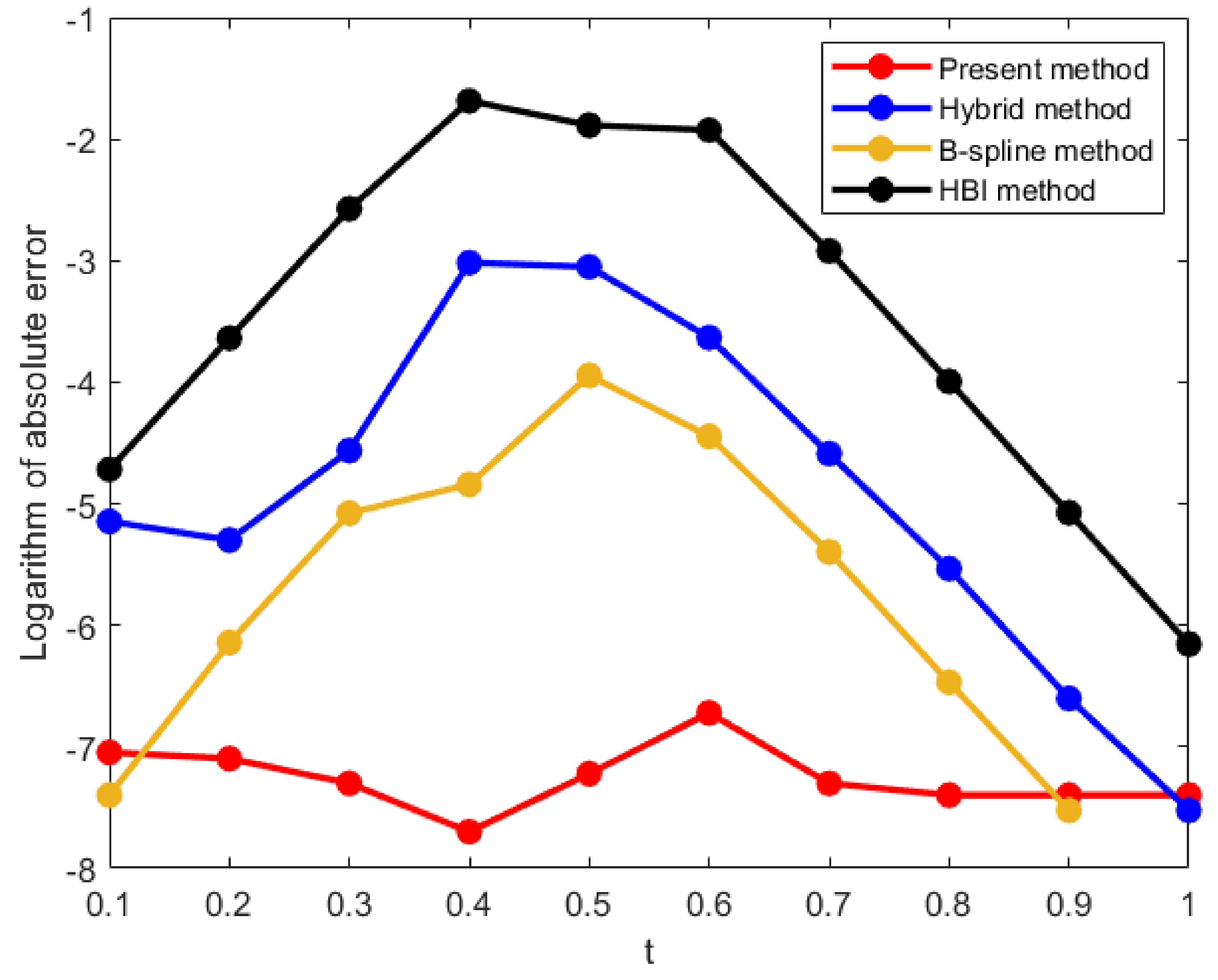
Figure 1.
Logarithm of absolute errors of at for Example 1.
Figure 1.
Logarithm of absolute errors of at for Example 1.
Figure 2.
Logarithm of absolute errors of at for Example 1.
Figure 2.
Logarithm of absolute errors of at for Example 1.
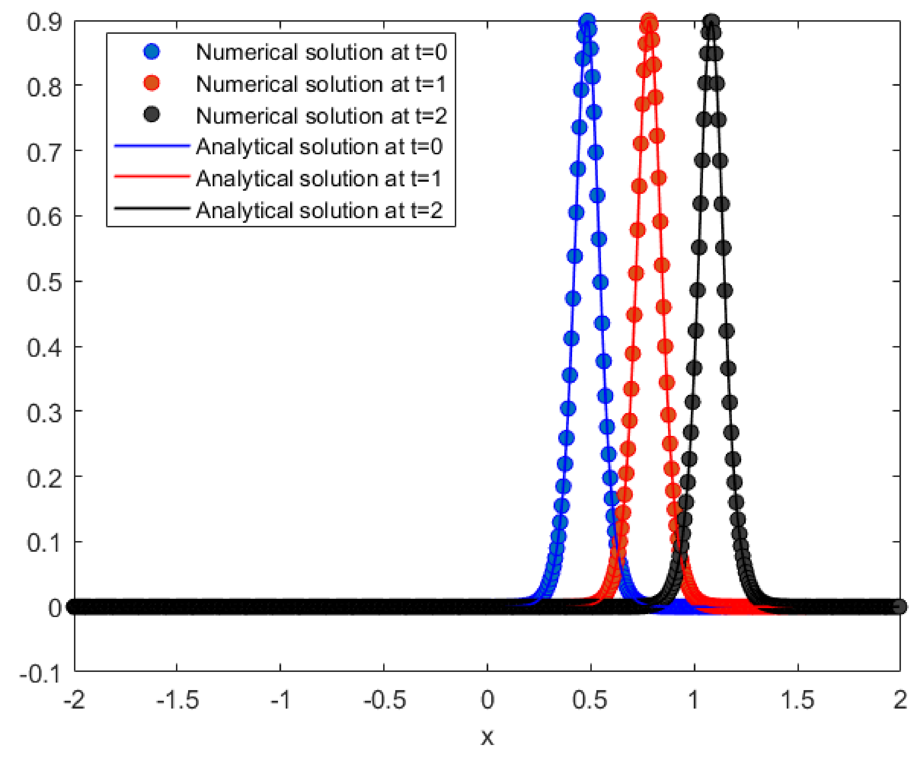
Figure 3.
Numerical solutions of obtained by the present method and analytical solutions at for Example 1.
Figure 3.
Numerical solutions of obtained by the present method and analytical solutions at for Example 1.
Figure 4.
Absolute error of obtained by the present method at for Example 1.
Figure 4.
Absolute error of obtained by the present method at for Example 1.
Figure 5.
Numerical solutions of vs. at , for Example 1.
Figure 5.
Numerical solutions of vs. at , for Example 1.
Figure 6.
Numerical solutions of vs. at , for Example 1.
Figure 6.
Numerical solutions of vs. at , for Example 1.
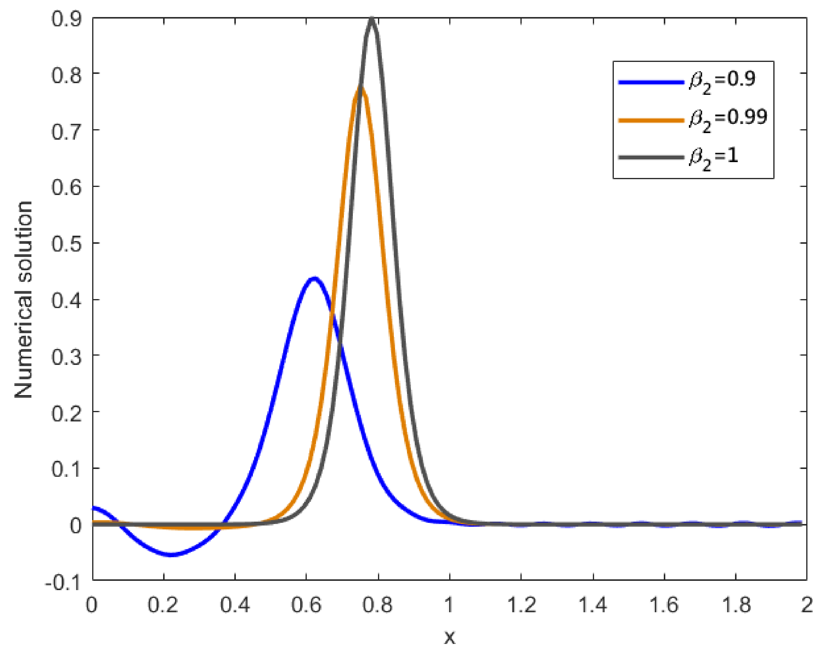
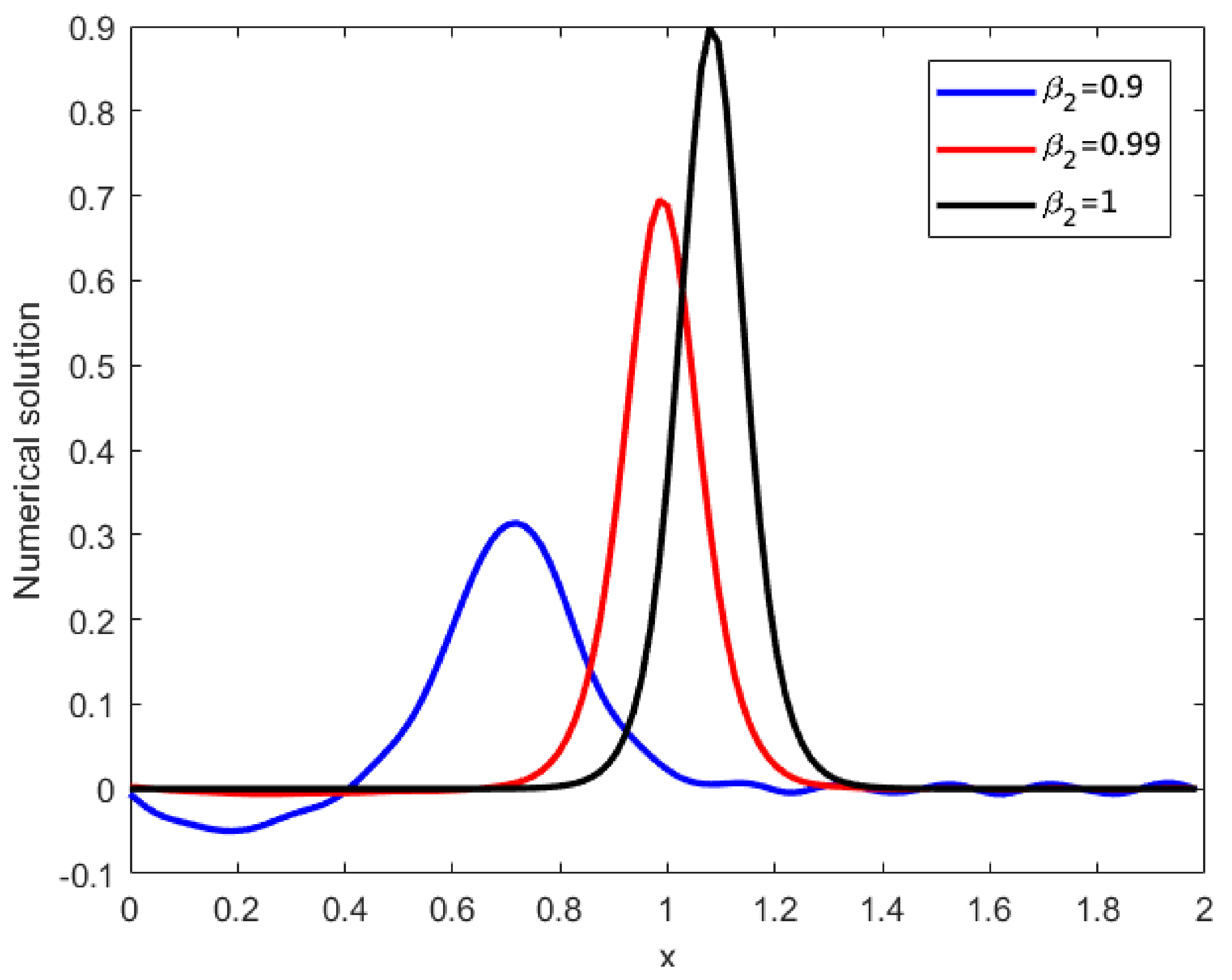
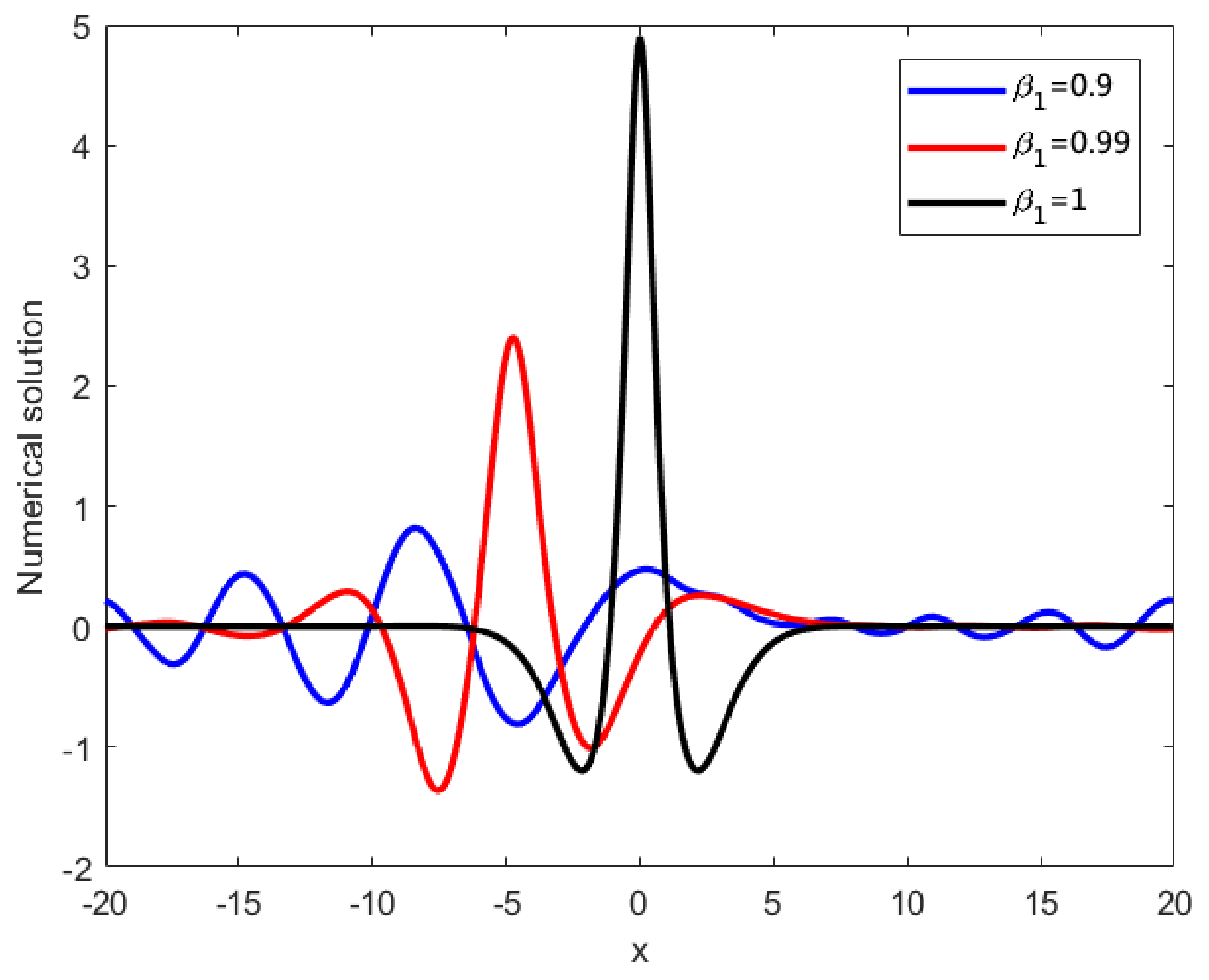
Figure 7.
Numerical solutions of vs. at different for Example 1.
Figure 7.
Numerical solutions of vs. at different for Example 1.
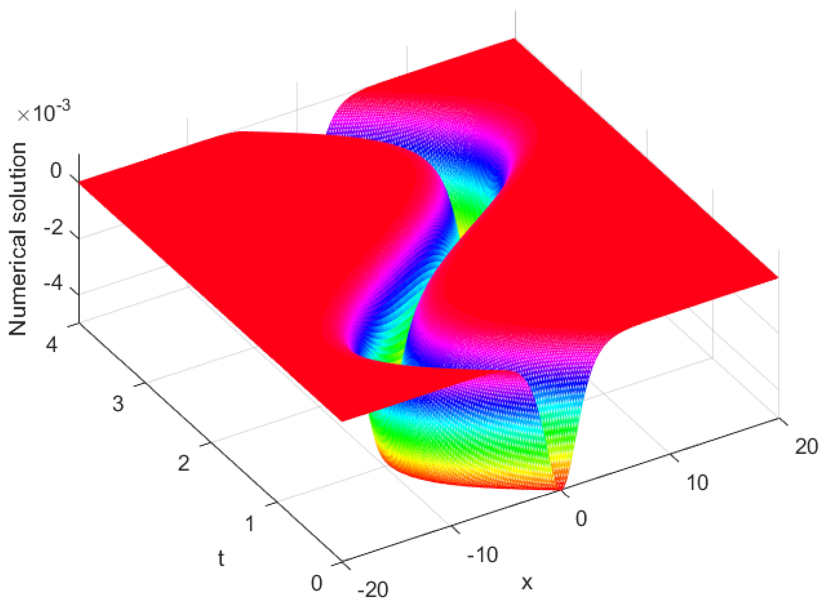
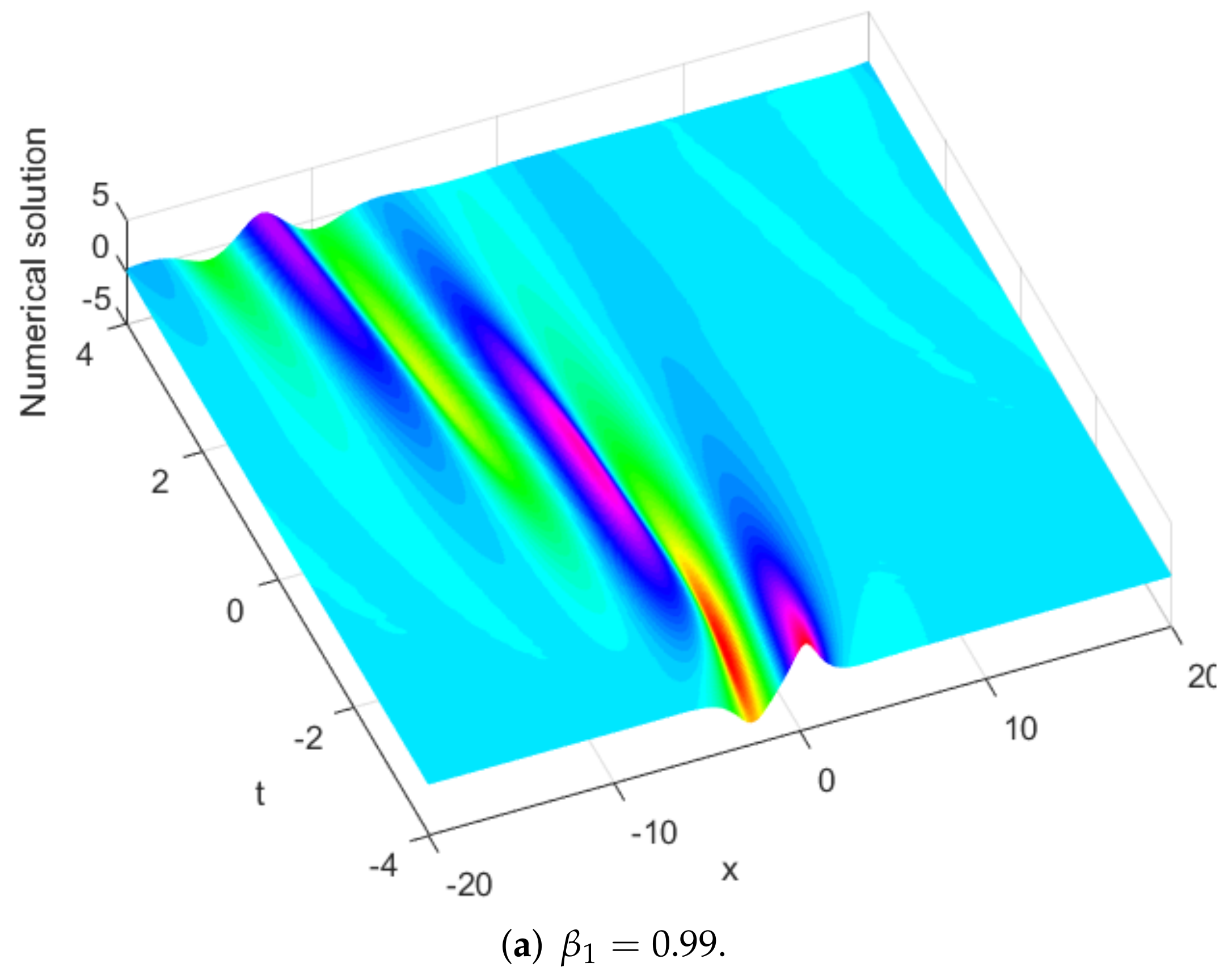
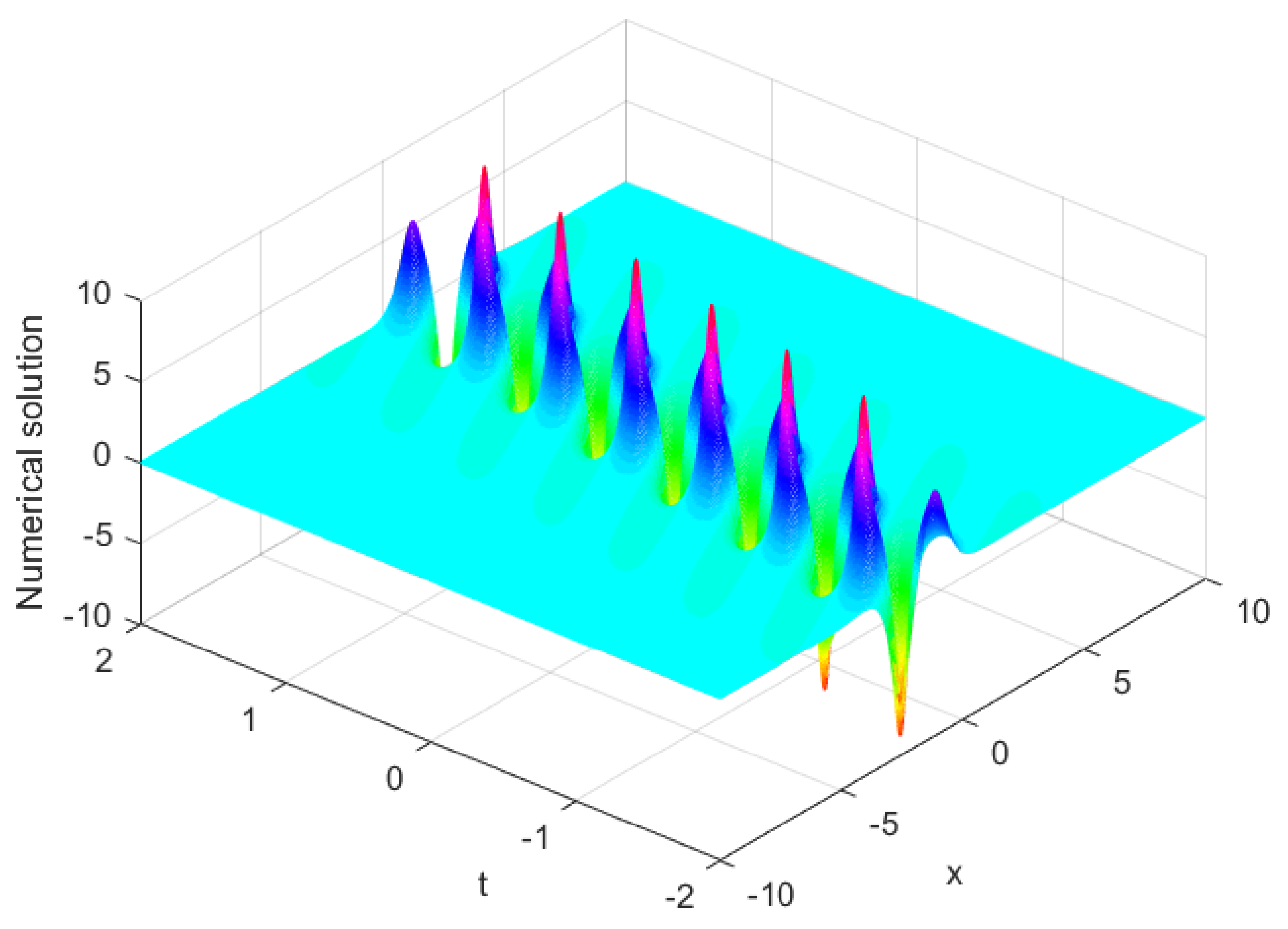
Figure 8.
Numerical solution of obtained by the present method for Example 2.
Figure 8.
Numerical solution of obtained by the present method for Example 2.
Figure 9.
2D contour plot of obtained by the present method for Example 2.
Figure 9.
2D contour plot of obtained by the present method for Example 2.
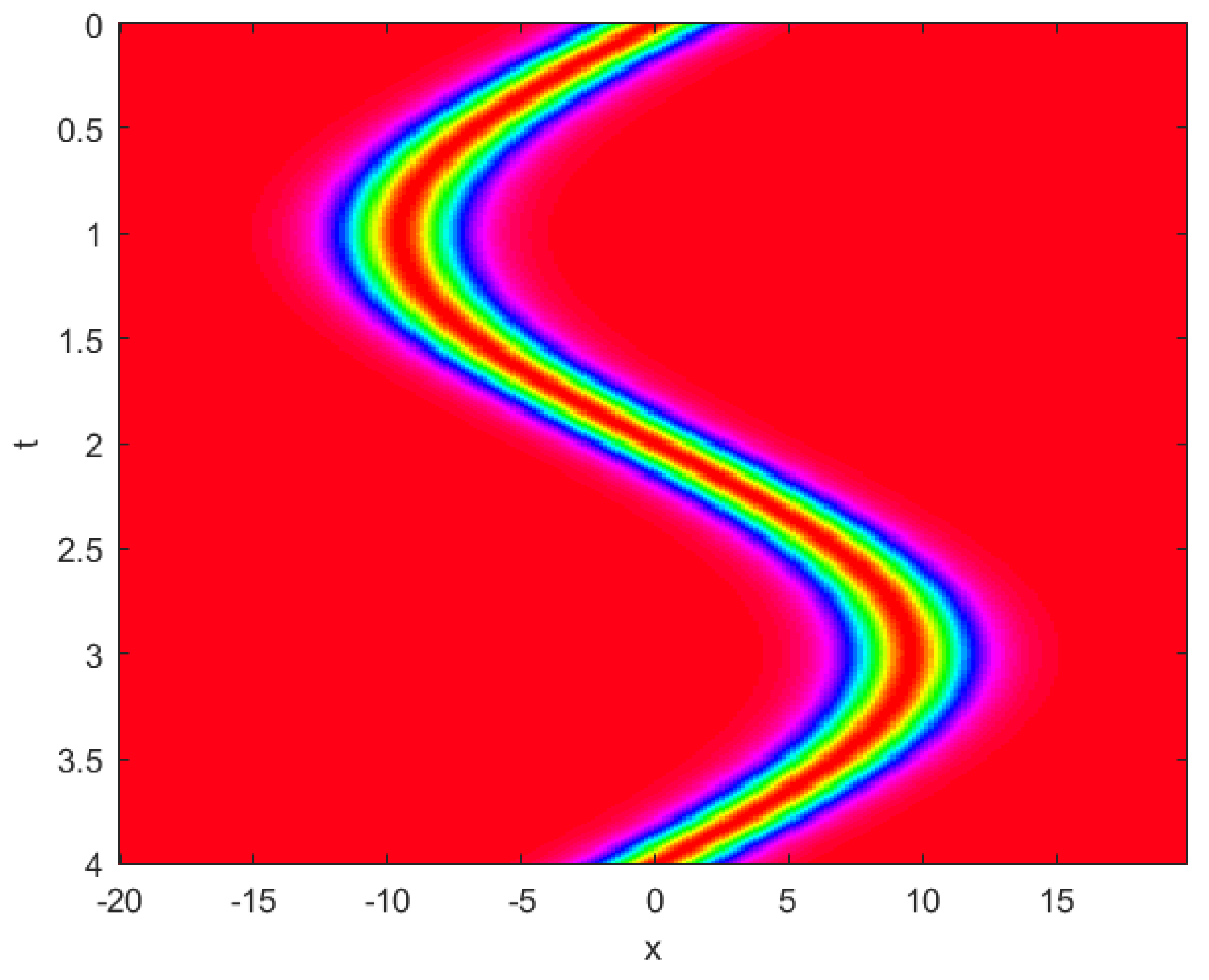
Figure 10.
2D density plot of obtained by the present method for Example 2.
Figure 10.
2D density plot of obtained by the present method for Example 2.
Figure 11.
Absolute errors of obtained by the present method at for Example 2.
Figure 11.
Absolute errors of obtained by the present method at for Example 2.
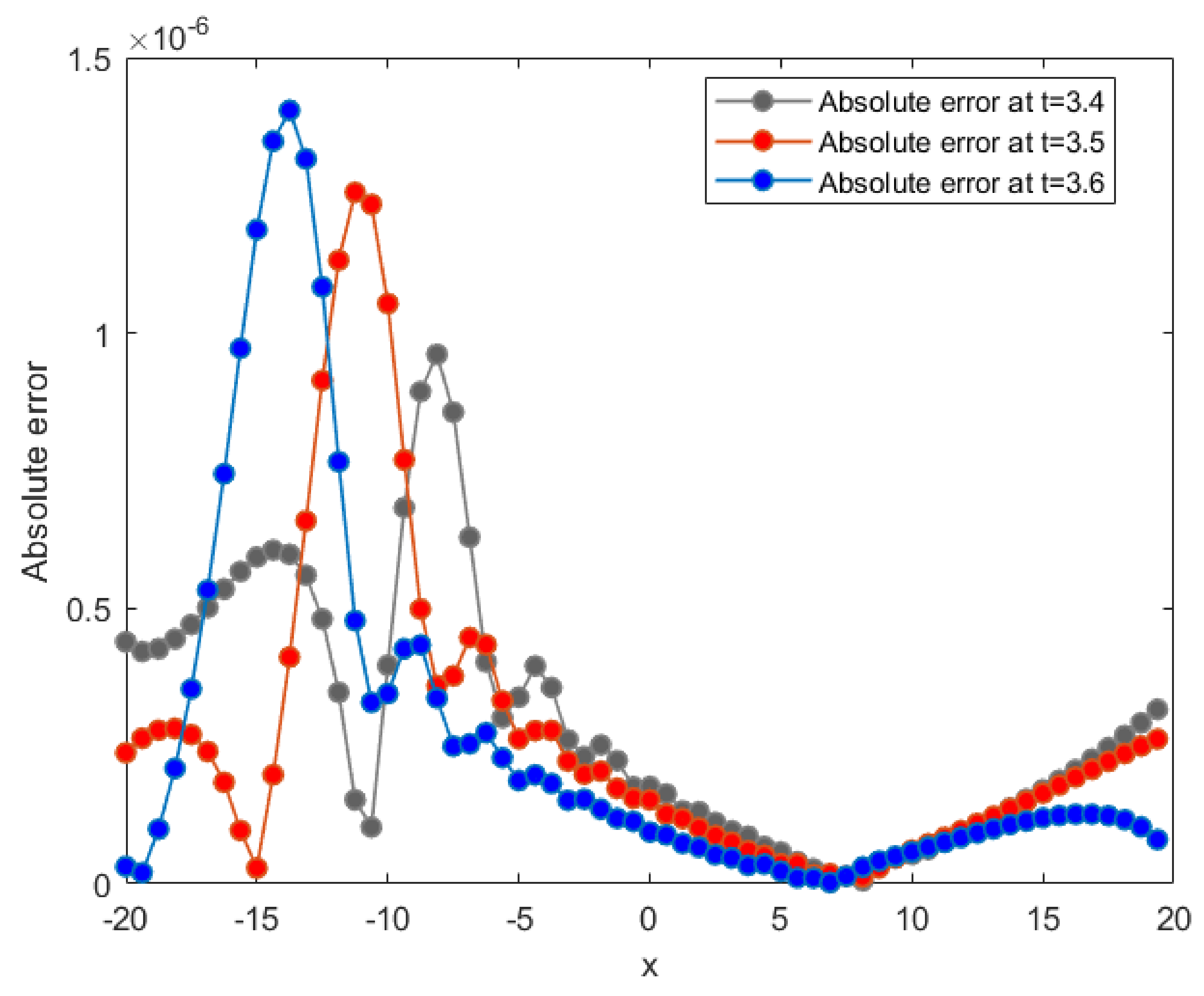
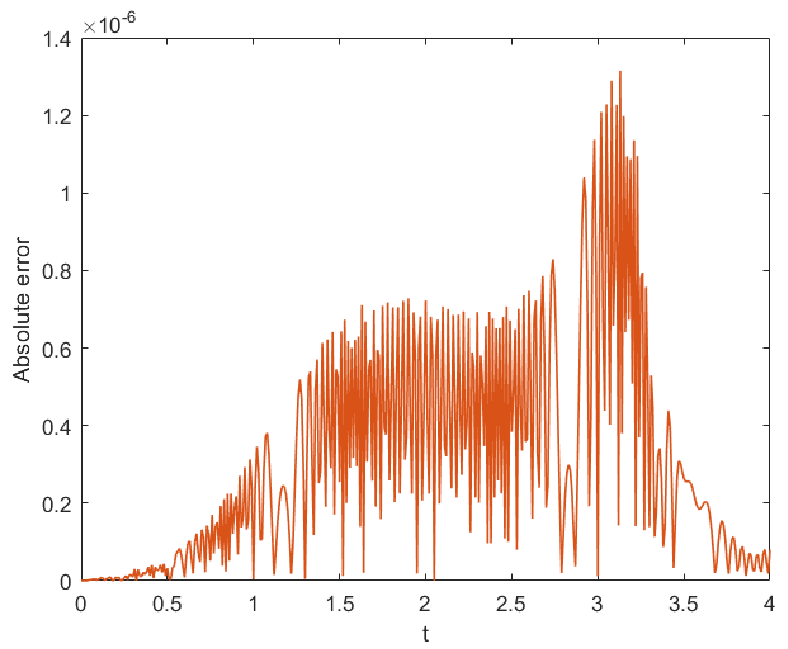
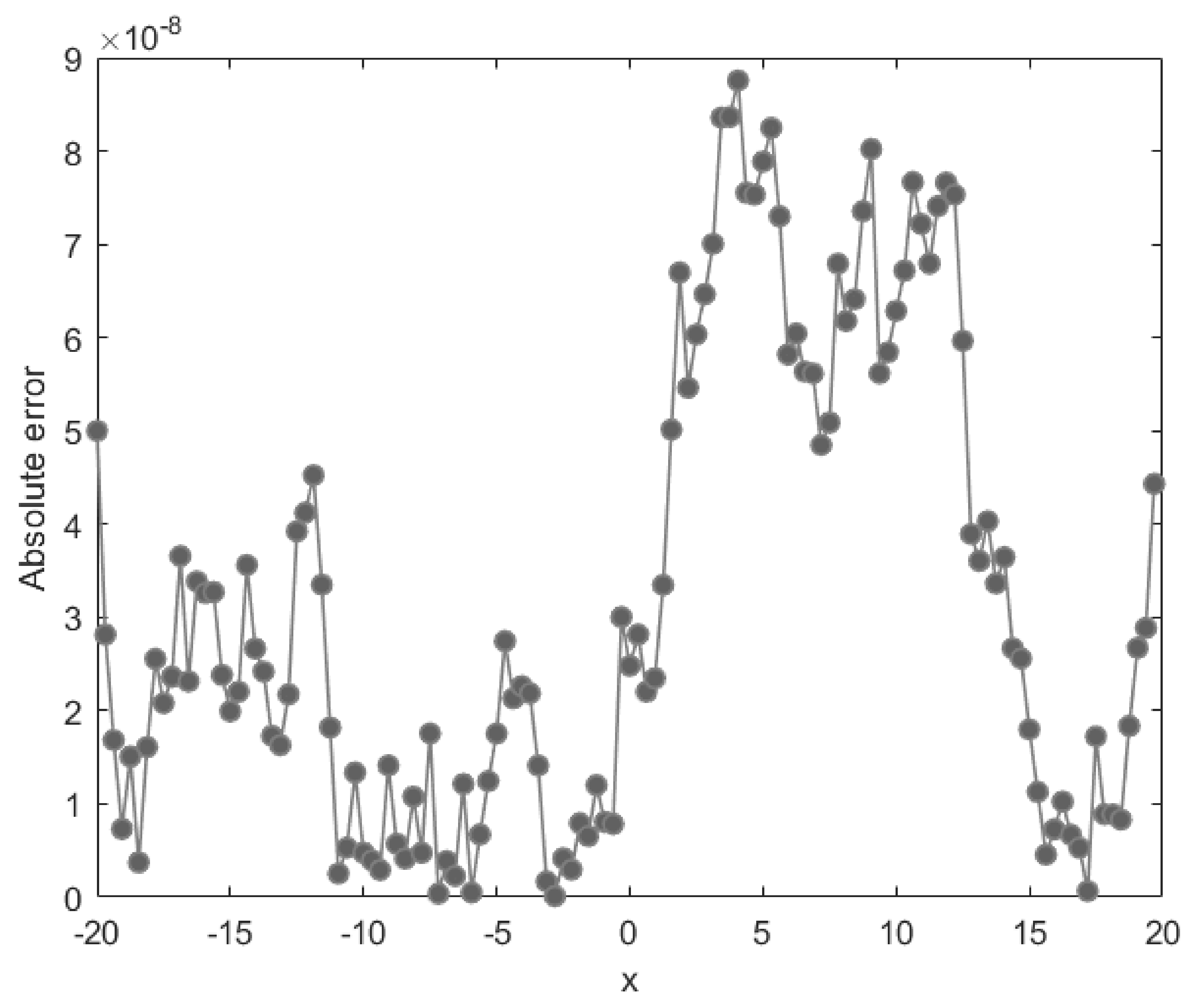
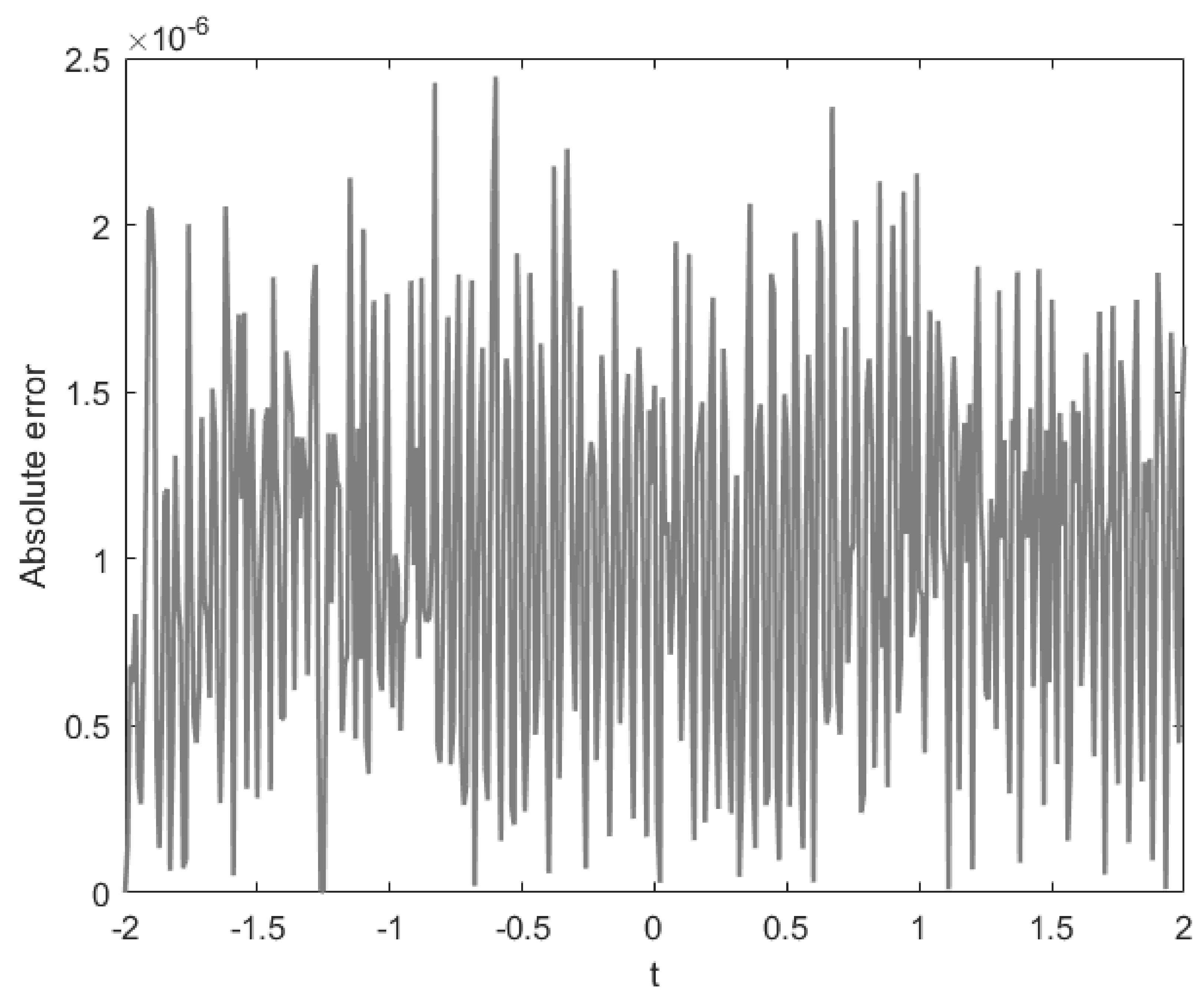
Figure 12.
Absolute error of obtained by the present method at for Example 2.
Figure 12.
Absolute error of obtained by the present method at for Example 2.
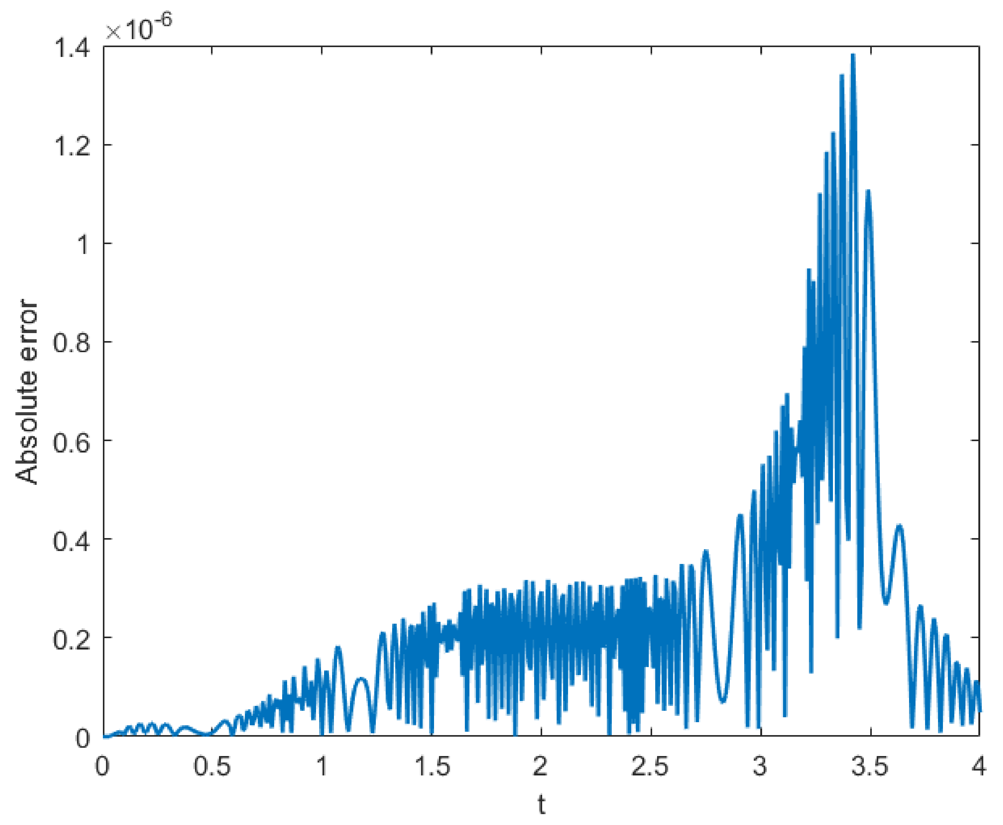
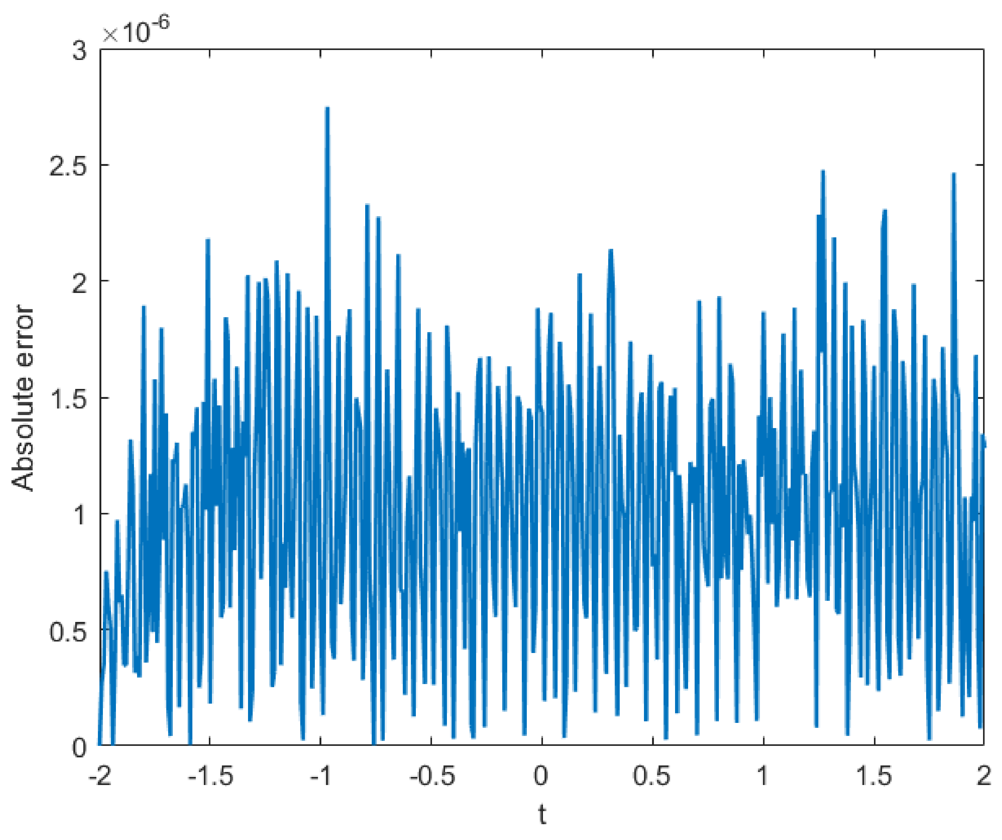
Figure 13.
Absolute error of obtained by the present method at for Example 2.
Figure 13.
Absolute error of obtained by the present method at for Example 2.
Figure 14.
Absolute error of obtained by the present method at for Example 2.
Figure 14.
Absolute error of obtained by the present method at for Example 2.
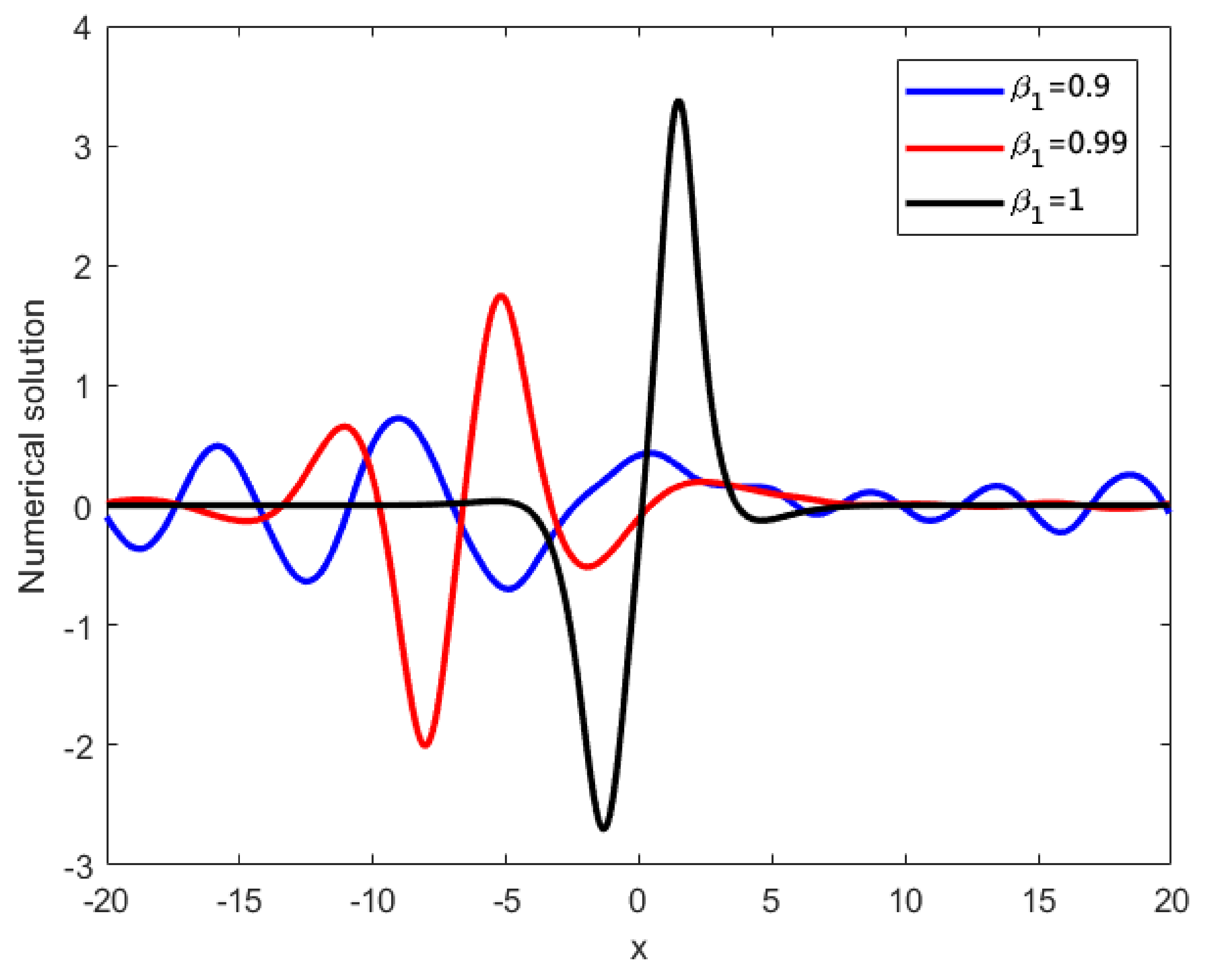
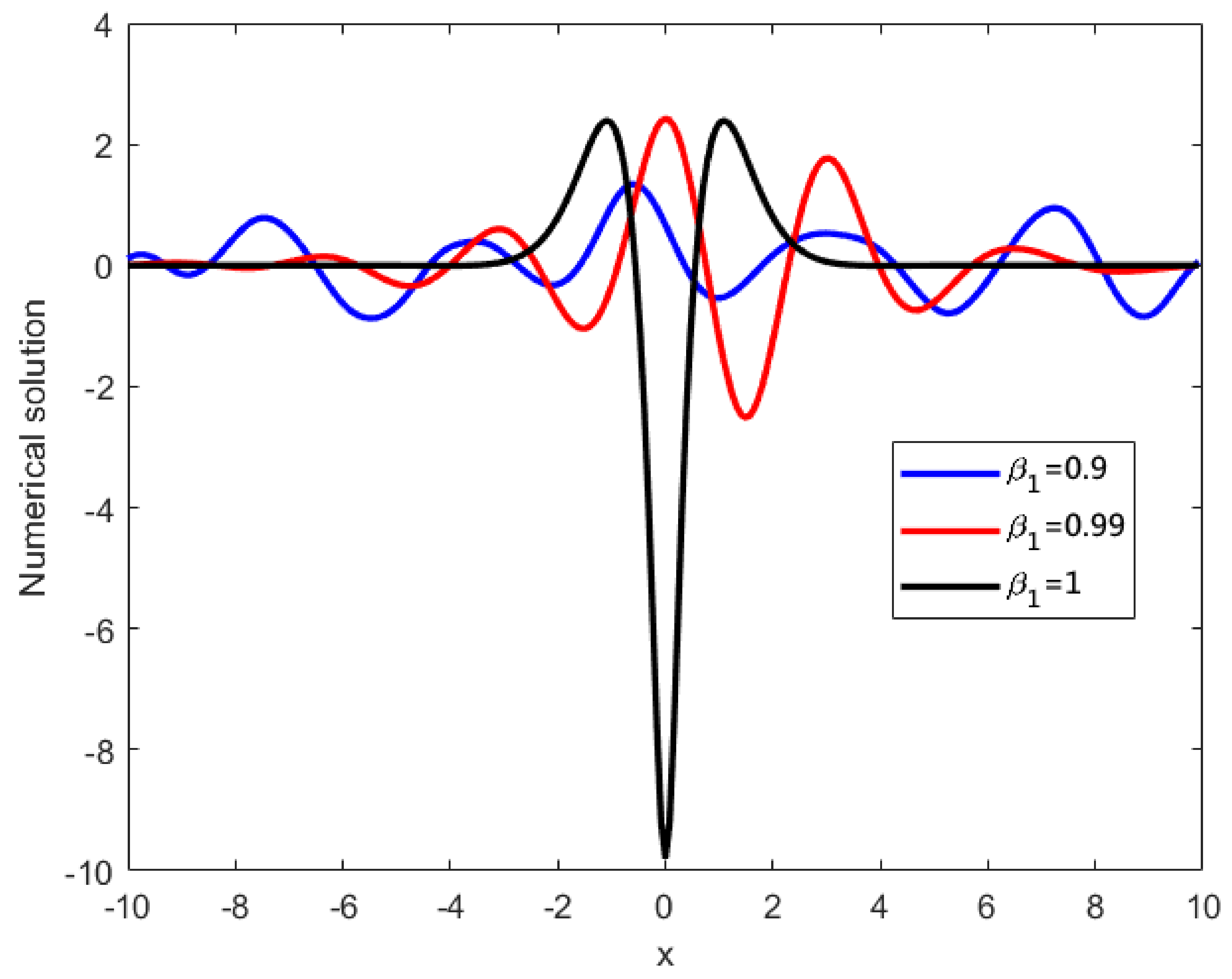
Figure 15.
Numerical solutions of vs. at different , for Example 2.
Figure 15.
Numerical solutions of vs. at different , for Example 2.
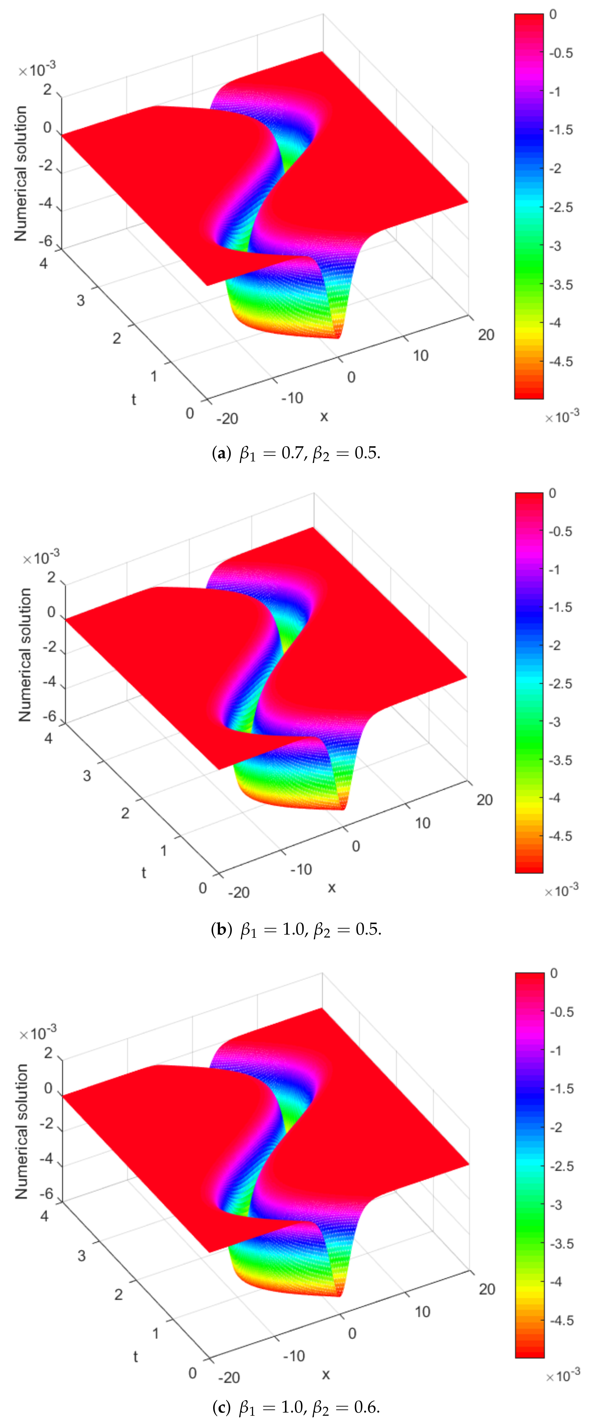
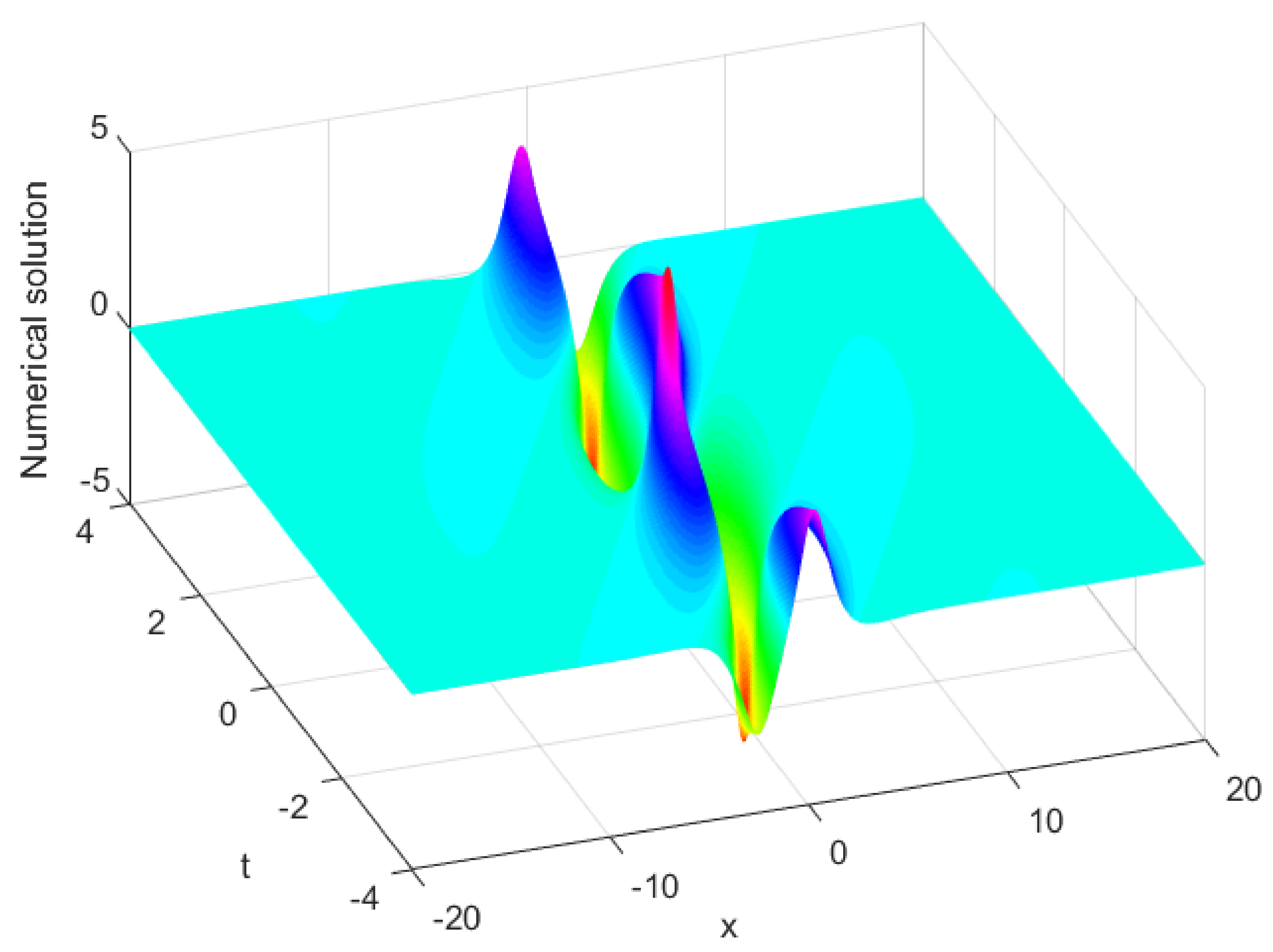
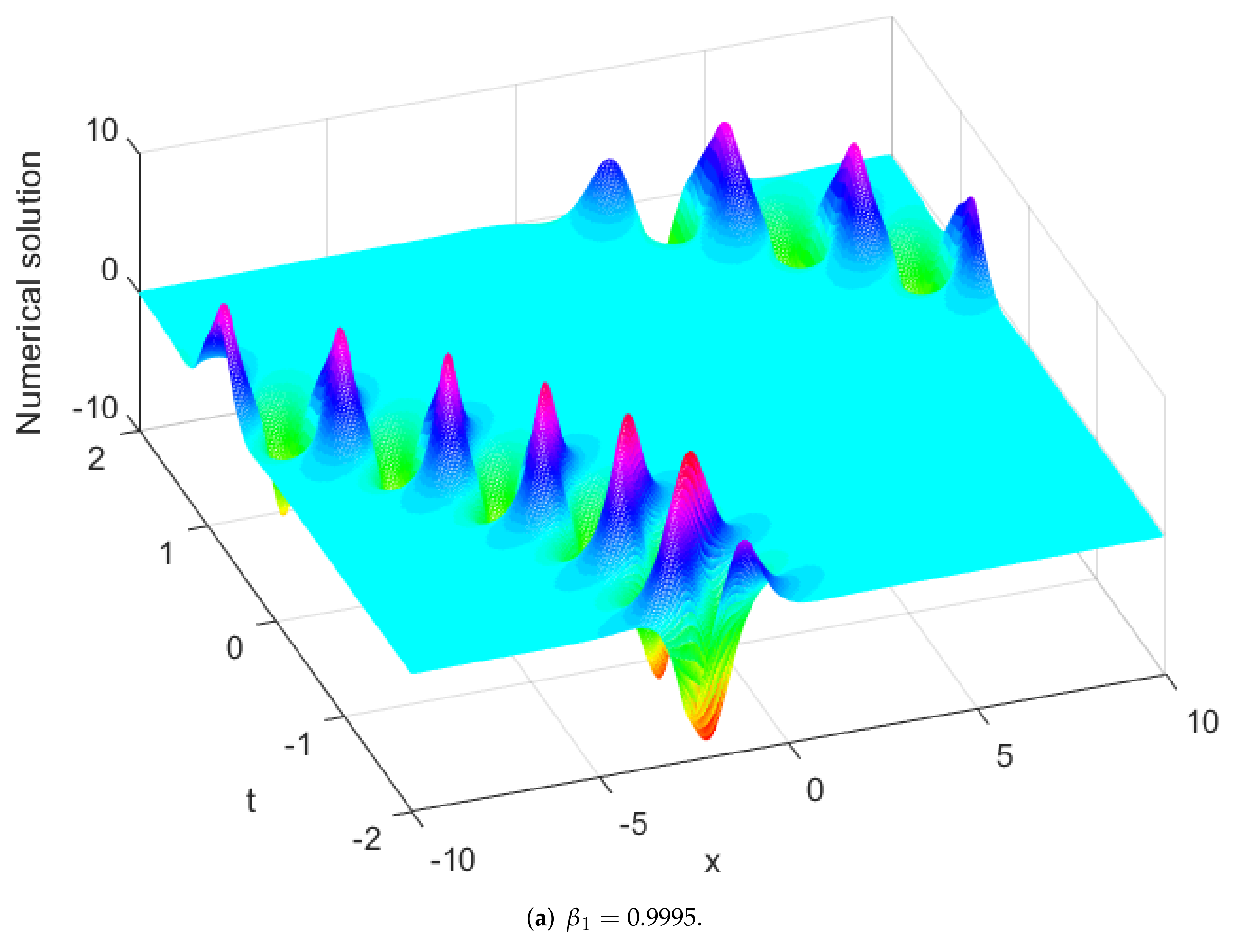
Figure 16.
Numerical solution at , , , for Example 3.
Figure 16.
Numerical solution at , , , for Example 3.
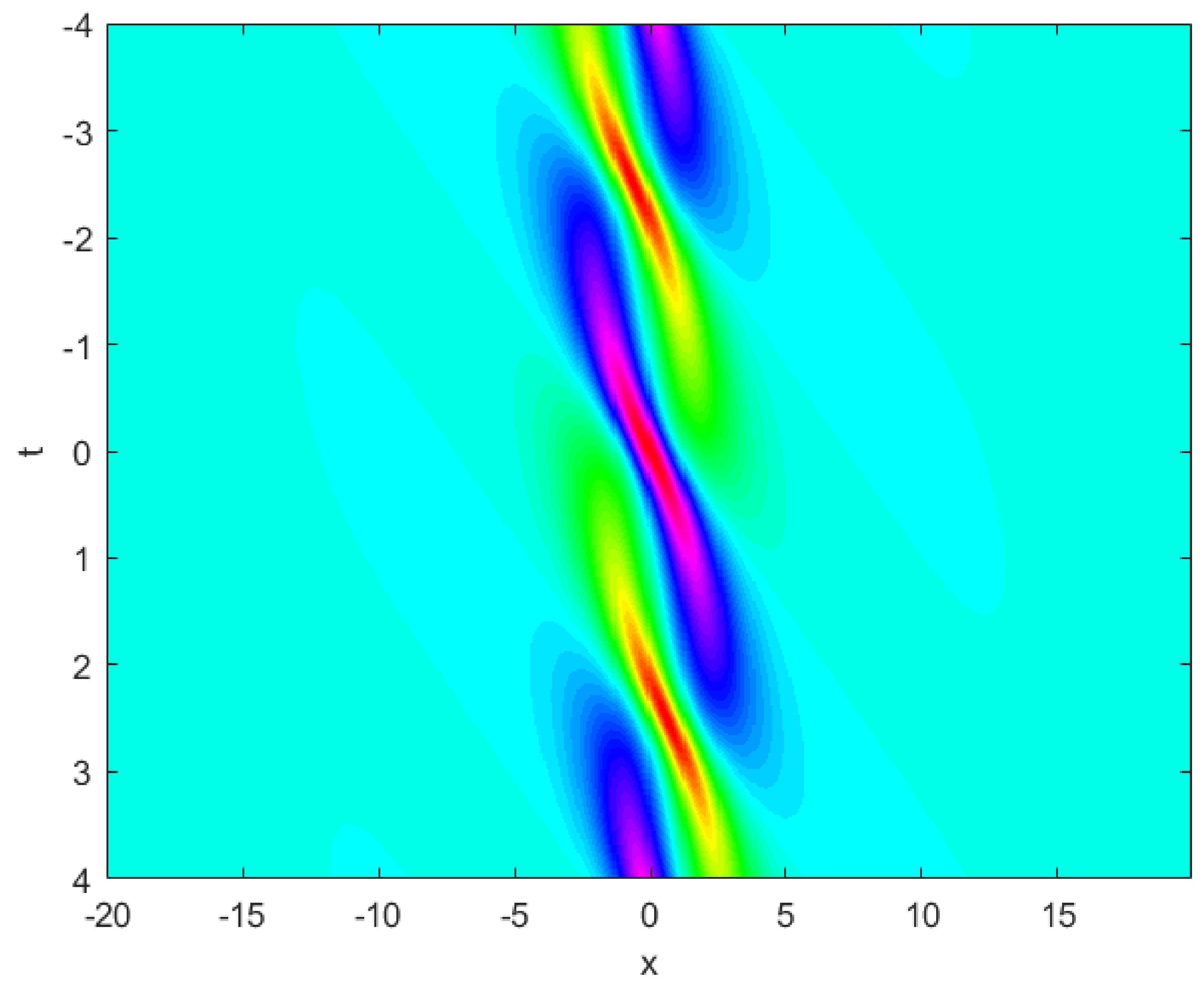
Figure 17.
2D contour plot at , , , for Example 3.
Figure 17.
2D contour plot at , , , for Example 3.
Figure 18.
2D density plot at , , , for Example 3.
Figure 18.
2D density plot at , , , for Example 3.
Figure 19.
Absolute error at , , , , for Example 3.
Figure 19.
Absolute error at , , , , for Example 3.
Figure 20.
Absolute error at , , , , for Example 3.
Figure 20.
Absolute error at , , , , for Example 3.
Figure 21.
Numerical solutions of vs. at , , , , , for Example 3.
Figure 21.
Numerical solutions of vs. at , , , , , for Example 3.
Figure 22.
Numerical solutions of vs. at , , , , , for Example 3.
Figure 22.
Numerical solutions of vs. at , , , , , for Example 3.
Figure 23.
Numerical solutions at , , , and different for Example 3.
Figure 23.
Numerical solutions at , , , and different for Example 3.
Figure 24.
Absolute error at , , , , for Case II.
Figure 24.
Absolute error at , , , , for Case II.
Figure 25.
Absolute error at , , , , for Case II.
Figure 25.
Absolute error at , , , , for Case II.
Figure 26.
Absolute error at , , , , for Case II.
Figure 26.
Absolute error at , , , , for Case II.
Figure 27.
Numerical solutions of vs. at , , , , , for Case II.
Figure 27.
Numerical solutions of vs. at , , , , , for Case II.
Figure 28.
Numerical solutions of vs. at different , , , , for Case II.
Figure 28.
Numerical solutions of vs. at different , , , , for Case II.
Figure 29.
Numerical solution of vs. at , , , for Case II.
Figure 29.
Numerical solution of vs. at , , , for Case II.
Figure 30.
2D contour plot of vs. at , , , for Case II.
Figure 30.
2D contour plot of vs. at , , , for Case II.
Figure 31.
2D density plot of vs. at , , , for Example 3.
Figure 31.
2D density plot of vs. at , , , for Example 3.
Table 1.
Spatial numerical errors , and their corresponding convergence rates at for Example 1.
Table 1.
Spatial numerical errors , and their corresponding convergence rates at for Example 1.
| N | | | | |
|---|
| 32 | | − | | − |
| 64 | | | | |
| 128 | | | | |
| 256 | | | | |
| 512 | | | | |
Table 2.
Comparison of absolute errors at .
Table 2.
Comparison of absolute errors at .
| x | Absolute Error |
|---|
| HBI [30]
| ANS [29]
| Hybrid [26] | B–Spline [27] | Present Method |
|---|
| | | | | |
| | | | | |
| | | | | |
| | | | | |
| | | | | |
| | | | | |
| | | | | |
Table 3.
Comparison of absolute errors at .
Table 3.
Comparison of absolute errors at .
| x | Absolute Error |
|---|
| HBI [30]
| ANS [29]
| Hybrid [26] | B–Spline [27] | Present Method |
|---|
| | | | | |
| | | | | |
| | | | | |
| | | | | |
| | | | | |
| | | | | |
| | | | | |
Table 4.
Comparison of of at , , , for Example 1.
Table 4.
Comparison of of at , , , for Example 1.
| t | | | | | |
|---|
| | | | | |
| | | | | |
| | | | | |
| | | | | |
| | | | | |
Table 5.
Error norms and at different times for Example 2.
Table 5.
Error norms and at different times for Example 2.
| | |
|---|
| Present Method
| Ref. [32]
| Present Method | Ref. [32]
|
|---|
| | | | |
| | | | |
| | | | |
| | | | |
Table 6.
Numerical results of obtained by the present method at for Example 2.
Table 6.
Numerical results of obtained by the present method at for Example 2.
| x | Analytical Solution | Numerical Solution | Absolute Error |
|---|
| | | |
| | | |
| | | |
| | | |
| | | |
| | | |
| | | |
| | | |
Table 7.
Numerical results of at ,, , , for Case I.
Table 7.
Numerical results of at ,, , , for Case I.
| x | Analytical Solution | Numerical Solution | Absolute Error |
|---|
| | | |
| | | |
| | | |
| | | |
| 0 | | | |
| | | |
| | | |
| | | |
Table 8.
Error norms, , and at , , , for Example 3.
Table 8.
Error norms, , and at , , , for Example 3.
| | | | | |
|---|
| | | | | |
| | | | | |
| | | | | |
Table 9.
Comparison of of at , , , for Example 3.
Table 9.
Comparison of of at , , , for Example 3.
| t | | | | | |
|---|
| | | | | |
| | | | | |
| 0 | | | | | |
| 1 | | | | | |
| 2 | | | | | |
Table 10.
Numerical results of at , , , , for Case II.
Table 10.
Numerical results of at , , , , for Case II.
| x | Analytical Solution | Numerical Solution | Absolute Error |
|---|
| | | |
| | | |
| | | |
| | | |
| | | |
| | | |
| | | |
| | | |
| | | |
Table 11.
Error norms, , and at , , , for Example 3.
Table 11.
Error norms, , and at , , , for Example 3.
| | | | | |
|---|
| | | | | |
| | | | | |
| | | | | |
Table 12.
Comparison of of at , , , for Example 3.
Table 12.
Comparison of of at , , , for Example 3.
| t | | | | | |
|---|
| | | | | |
| 0 | | | | | |
| 1 | | | | | |
| 2 | | | | | |


