Article

Fixed-Time Fractional-Order Global Sliding Mode Control for Nonholonomic Mobile Robot Systems under External Disturbances

1
UMR 8201, CNRS, LAMIH, INSA Hauts-de-France, Université Polytechnique Hauts-de-France, F-59313 Valenciennes, France
2
Department of Computer & Networks Engineering, College of Computer Science and Engineering, University of Jeddah, P.O. Box 34, Jeddah 21959, Saudi Arabia
*
Author to whom correspondence should be addressed.
Fractal Fract. 2022, 6(4), 177; https://doi.org/10.3390/fractalfract6040177
Submission received: 14 January 2022 / Revised: 15 March 2022 / Accepted: 18 March 2022 / Published: 22 March 2022

Abstract

:
The present study addresses the problem of fixed-time stabilization (FTS) of mobile robots (MRs). The study’s distinguishing aspects are that the system under examination is subjected to external disturbances, and the system states are pushed to zero in a finite time. This paper suggests new control techniques for chained-form nonholonomic systems (CFNS) subjected to disturbances. First, a switching fractional-order (FO) control approach is proposed for a first-order subsystem (FOS) of an MR under complex disturbances. Secondly, an FO generic global sliding mode control approach is designed for the second-order system (SOS) of the MR in the presence of disturbances. The suggested sliding manifold for the SOS of the MR guarantees global system stability and reduces the chattering problem during control operations. A conventional quadratic Lyapunov function (QLF) is used to converge to the origin in a finite time (FnT). Through this study, a stabilizer for an MR in the presence of disturbances based on an FO switching time-varying controller that can stabilize immeasurable states in a fixed time is proposed. Finally, three case simulations are provided to demonstrate the efficacy of the control strategy proposed in this work against external disturbances.

1. Introduction

In recent years, a growing body of research on robotic building has revealed a number of benefits including increased safety, faster construction, and better quality control [1,2]. Construction robots, however, have had a slow acceptance rate [2]. As a consequence, the anticipated benefits have not been realized, which is problematic in an era when mass-scale building and remodeling with high levels of efficiency and quality is in great demand [2]. The fourth industrial revolution brought a wave of change to logistics. Since the beginning of human society, transportation has been one of the most urgent concerns [2]. There are a variety of applications for diverse tasks that are all targeted at enhancing processes and, as a result, production and volume [3]. Some logistics-related collaborative robots can even be taught to execute tasks. This reduces unused programming time and speeds up the bespoke packaging process. The logistics and transportation industries are being progressively infiltrated by robots [3].
Stabilization of nonholonomic systems (SNS) has attracted a great deal of interest in recent years due to its practical applications in various fields sych as wheeled vehicles and mobile robotics. Controlling MRs, however, is difficult due to the fact that the number of control inputs is smaller than the degrees of freedom [4]. Stationary continuous feedback cannot be stabilized in this type of robot [5,6]. Furthermore, certain complex situations with regard to these MRs in terms of initial conditions make stabilization more complicated [4,7].
The problem of SNS becomes more difficult in the presence of external disturbances [8]. To solve these difficulties, several control techniques have been proposed in the literature, including output feedback control and adaptive state feedback techniques [9,10,11], exponential regulation [12], and global robust stabilization [13,14]. Recently, the concept of finite-time controllers for nonholonomic systems was presented in [7,15,16,17,18]. Finite-time stability (FnTS) is more powerful than traditional asymptotic stability. FnTS usually has higher accuracy, a faster convergence rate, and higher resilience. In [19], the FnT stabilization problem of nonholonomic systems with output constraints was investigated. The authors of [19] proposed output feedback for an MR using an FnT control technique with input saturation. The work developed in [19] addressed the design of the finite-time feedback controller and observer.
Recently, many researchers have addressed the problem of the fixed-time stabilization of these MRs, which are characterized by a fixed-time convergence [20,21]. The authors of [21] proposed output feedback for uncertain NSs using a fixed-time control. The work reported in [20] involved the development of a new switching time-varying observer capable of estimating immeasurable states in a fixed time, allowing us to design an output feedback controller.
The theory of integrals and derivatives of any real or complex order has progressed with the development of fractional calculus. Many studies have been reported in the literature that combine the fractional order with sliding mode control (SMC) to increase the performance stabilization of dynamical systems. The authors in [22,23] proposed an FO-SMC technique for controlling nonlinear dynamical systems by choosing the specific sliding variables that are used to achieve the FnTS. However, stabilization of MR systems in the presence of disturbances is more commonly addressed using FO controllers. In addition, by combining FO fixed-time controllers and SMC, the controller becomes more robust against disturbances and provides more degrees of freedom. To the best of our knowledge, however, there is no literature describing the fractional-order fixed-time control method for mobile robots. This paper addresses the design of fixed-time FO controllers for mobile robots in the presence of disturbances. Fractional calculus, in fact, opens up new possibilities for controller design. Compared to integer-order controllers, fractional-order controllers offer more opportunities to improve control performance and resilience [24]. Furthermore, fractional-order controllers can aid in the stabilization of dynamical systems [25].
In this paper, two new FO first/second-order fixed-time convergent controllers are designed for an MR subjected to external disturbances to its global stabilization convergence time. The considered controllers are based on the FO-SMC [23,26,27,28,29], with fixed-time control techniques [30], which are particularly suitable for this situation as a robust rejection of disturbances is achieved. The robustness is studied for various cases in terms of disturbances and the initial conditions. We are concerned with fixed-time stabilization via state feedback for a type of uncertain chained-form nonholonomic system with FO in this study, as part of our ongoing research. The key contributions of this study are as follows, compared to similar existing results in the literature:
  • The fixed-time convergence is fully addressed in this work, taking into consideration real system needs.
  • In contrast to previous finite-time/fixed-time control methods, the present paper combines fixed-time control and fractional theory.
  • Two FO fixed-time controllers are designed for first/second order systems, and two switching strategies are suggested to ensure the fixed-time stability of uncertain chained-form nonholonomic systems.
  • The second-order controller proposed in this work possesses better performance with regard to reduction of the chattering phenomenon and global stabilization.
  • The theory results are confirmed by numerical results for various cases and are compared with recent fixed-time controls [30].
Some basic properties, definitions, and lemmas on fractional calculus and fixed-time stability are presented in Section 2. Section 3 gives the main results. Numerical simulation results are reported in Section 4. A conclusion is presented in Section 5.
Z + and R + are the sets of integer numbers and positive real numbers, respectively. Throughout the paper, while C and R represent separately the set of complex real numbers, R n denotes the n-dimensional Euclidean space. For a vector ϑ = [ ϑ 1 , ϑ 2 , , ϑ n ] T R n , we use ϑ 2 = i = 1 n | ϑ i | 2 to denote the two-norm of vector ϑ , while || ϑ || represents an arbitrary norm of vector ϑ .

2. Preliminaries and Conceptualization of the Problem

2.1. Preliminary Considerations on Fractional Calculus

The Caputo derivative is the most frequently used fractional-order derivative of Y ( t ) , given as [31,32,33]:
a C D t a Y ( t ) = 1 Γ ( a β ) a t Y ( β ) ( τ ) ( t τ ) a β + 1 d τ
where β N * , a denotes the order of the derivative such that ( β 1 ) < a < β , and Γ ( . ) is the gamma function, which is defined by the following equation:
Γ ( ζ ) = 0 e t t ζ 1 d t ,
The Caputo operators [31,33] are usually the two definitions of the fractional-order derivative used.
Property 1.
Equation (3) applies to the Caputo derivative
t 0 C D t a ( t 0 C D t λ Y ( t ) ) = t 0 C D t a λ Y ( t )
where a λ 0 .
Property 2.
If 0 < a < 1 , we can write (4) the Caputo derivative
t 0 C D t 1 κ ( t 0 C D t a Y ( t ) ) = t 0 C D t a ( t 0 C D t 1 κ Y ( t ) ) = Y ˙ ( t )
Throughout this article, the notation C D a for the Caputo operator will be substituted with D κ .

2.2. Preliminary Considerations for Finite/fixed-Time Stability

We take the system below:
x ˙ = Θ ( x ; Ψ )
where x R n is the state variable of the system in (5). The notation Ψ is a constant parameter of the system in Equation (5).
The function Θ ( x ; Φ ) : R n R n is nonlinear, and the origin is considered to be an equilibrium point in the system in Equation (5). Its initial conditions are x 0 = x ( 0 ) R n .
Definition 1.
[34,35] If there is such a thing as a function Φ T : R n R + , the origin of (5) is globally finite-time stable. Thus, the solution Ψ ( t , x 0 ) of the system in (5) reaches the point of equilibrium in a certain amount of time. Hence, the settling time function can be defined as t [ 0 , Ψ ( x 0 ) ] , for t Φ T ( x 0 ) , Θ ( x 0 , t ) = 0 .
Definition 2.
[34,35] It is a globally fixed-time equilibrium if the system in Equation (5) is globally finite-time stable and the settling-time expression is Φ T ( x 0 ) is limited by a positive value Φ T M a x > 0 .
To explain finite-time stability in the face of rapid temporal convergence, Lemmas 1 and 2 are used.
Lemma 1.
[36] Consider the notation Π ( t ) as the Lyapunov function (LF) given by the following equation:
Π ˙ ( t ) ϖ 1 Π ( t ) ϖ 2 φ ς ( t ) , t 0 , φ ( t 0 ) 0
where, ϖ 1 > 0 , ϖ 2 > 0 , φ 0 is the initial value of Π ( t ) , and 0 < ς < 1 . Let Π ( t ) , t > t 1 , then following a basic calculation, t s is,
t s = t 0 + 1 ϖ 1 ( 1 ς ) l n ϖ 1 φ 1 ς ( t 0 ) + ϖ 2 ϖ 2
Lemma 2.
[37] Consider LF Π ( t ) with initial value φ 0 as
Π ˙ ( t ) ϖ 1 Π ( t ) , t 0 , φ ( t 0 ) 0
where, ϖ 1 > 0 and 0 < ς < 1 . Let Π ( t ) , t > t 1 .
Then, the corresponding settling time t s can be given as
t r t 0 + ϖ 1 φ 1 ς ( t 0 ) ν a ( 1 ς )
Lemma 3.
[34] For the system in Equation (5), if there is a C 1 and φ ( x ) positively defined on a neighborhoodof the origin A ^ , with A ^ A , where Y x , Y y > 0 , 0 < Θ 1 < 1 , and Θ 1 > 0 such that φ ˙ ( x ) Y x φ θ 1 ( x ) Y y φ θ 2 ( x ) , then the origin of the system in (5) is fixed-time stable and the settling time Φ T ( x 0 ) satisfies ϕ T ( x ) Φ T M a x : = 1 Y x ( 1 Θ 1 ) + 1 Y y ( 1 Θ 2 ) , for all x A ^ .

2.3. Problem Formulation

Consider the MR presented in Figure 1, which is riding a unicycle. It has two driving wheels controlled by two actuators each, as well as one passive wheel that keeps the plane from flipping over while in motion. The position of the center of mass ( x , y ) is at the intersection of a straight line passing between the robot’s center and the axes of the two driving wheels. This MR’s configuration is as follows:
Y ( t ) = [ x y θ ] T ,
The heading angle of the MR is denoted by θ . The following equation gives the non-slipping and pure rolling conditions:
sin ( θ ) x ˙ cos ( θ ) y ˙ = 0 .
Under nonholonomic restrictions, the kinematics of the wheeled MR are as follows:
x ˙ = cos ( θ ) ν y ˙ = sin ( θ ) ν θ ˙ = ω
The angular/linear velocities are denoted, respectively, by the notations ω ( t ) / ν ( t ) .
Let us make the following changes.
ε 0 = x ( t ) ε 1 = y ε 2 = tan ( θ ) τ 0 = ν cos ( θ ) τ 1 = ω sec 2 ( θ )
Using the transformation, system (11) can be described as:
ε ˙ 0 = τ 0 + d 0 ε ˙ 1 = τ 0 ε 1 ε ˙ 2 = τ 1 + d 1
where d 0 and d 1 are unknown perturbations.

3. Main Results

This section describes a constructive approach for designing the FxT stabilizer of (13) in the face of perturbations, at any time T > 0 . At τ 0 , we start by choosing an appropriate non-zero constant input ρ . As a result, the ε -subsystem may be thought of as a nonlinear control, for which the fixed-time stabilizing controller was created. We propose a novel FO controller τ to fixed-time stabilize the ε 0 -subsystem after τ 0 reaches zero before a defined time and remains at zero.

3.1. Stabilization of the First-Order System (FOS) of the MR in the Presence of Perturbation

The FxTS of the first-order system of the CFD is presented in this subsection. The switching controller presented in the following proposition ensures the fixed-time stability of the FOS under perturbations.
Proposition 1.
Consider an FOS with the following switching control scheme:
τ 0 = ρ i f t T 1 Ξ 0 | ε 0 | γ 1 s i g n ( ε 0 ) Ξ 1 | ε 0 | γ 2 s i g n ( ε 0 ) Ξ 2 s i g n ( ε 0 )
where Ξ i is a positive constant. Then, the ε 0 -subsystem is fixed-time stable.
Proof. 
The candidate Lyapunov function (CLF) is selected as:
V ε 0 = 1 2 ε 0 2
The time-derivative of V ε 0 is given by:
V ˙ ε 0 = Ξ 0 | ε 0 | γ 1 + 1 Ξ 1 | ε 0 | γ 2 + 2 Ξ 2 | ε 0 |
      Ξ 0 ( 2 V ε 0 ) γ 1 + 1 2 Ξ 1 ( 2 V ε 0 ) γ 2 + 1 2 Ξ 2 ( 2 V ε 0 ) 1 2
Ξ 0 ( 2 V ε 0 ) γ 1 + 1 2 Ξ 1 ( 2 V ε 0 ) γ 2 + 1 2
We define the new variables as Y ϕ 1 = 2 Ξ 0 , Y ϕ 2 = 2 Ξ 1 , Y θ 1 = γ 1 + 1 2 , Y θ 2 = γ 2 + 1 2 .
Then, (18) becomes
V ˙ 0 ( t ) Y ϕ 1 V 0 ( t ) Y θ 1 Y ϕ 2 V 0 ( t ) Y θ 2
The ε 0 -subsystem is fixed-time stable based on Lemma 3. □
The FOS with matching perturbation is stabilized using a simple switching controller in this subsection. Based on this controller and using FO operators, a new control technique is designed in the next subsection.

3.2. Stabilization of the (FOS) of the MR Based on FO Control Method in the Presence of Perturbation

An FO-FxT switching control law (FO-FxT-SCL) is suggested for the optimization of the FOS of the MR under perturbations, based on t 0 D t λ s i g n ( ε ) . The first property of t 0 D t λ s i g n ( ε ) ensures that the output is within an arbitrarily small neighborhood of the optimal operating point and stays close to it thereafter in the FO-FxT-SCL. The second attribute has the potential to increase the control performance (i.e., convergence speed and accuracy). The changes in t 0 D t λ s i g n ( ε ) , 0 λ < 1 with regard to λ and t are depicted to demonstrate how the FO sign function’s characteristics lead to improved tracking behavior.
Lemma 4
([38]). Considering the Caputo fractional derivative t 0 D t λ φ ( t ) = 1 Γ ( 1 λ ) d d t 0 t φ ( τ ) ( t τ ) λ d τ , 0 λ < 1 , and the sign function, we obtain
t 0 D t λ s i g n ( ε ( t ) ) = > 0 , i f ε ( t ) > 0 , t > 0 < 0 , i f ε ( t ) < 0 , t > 0
Remark 1.
Consider the following scenarios: (i) for ε > 0 , we have t 0 D t λ s i g n ( ε ) = t λ Γ ( 1 λ ) ; (ii) for ε < 0 , we also have t 0 D t λ s i g n ( ε ) = t λ Γ ( 1 λ ) . In both situations, D t λ s i g n ( ε ) is bounded. Because the absolute value in the aforementioned situations is higher than that of the other cases, D t λ s i g n ( ε ) , ε is bounded, i.e., there exists an > 0 such that | D t λ s i g n ( ε ) | < .
Theorem 1.
Consider the FOS with the following switching control scheme:
τ 0 = ρ i f t T 1 Ξ 0 D λ 1 { | ε 0 | γ 1 s i g n ( ε 0 ) } Ξ 1 D λ 2 { | ε 0 | γ 2 s i g n ( ε 0 ) } Ξ 2 D λ 3 { s i g n ( ε 0 ) }
with 0 < λ i < 1 and λ i < γ i . Then, the ε 0 -subsystem is fixed-time stable. Then, ε 0 = 0 is Mittag–Leffler stable. If the assumption applies globally to R n , then ε 0 = 0 is globally fixed-time Mittag–Leffler stable.
Proof. 
The candidate Lyapunov function (CLF) is selected as:
V ε 1 = 1 2 ε 0 2
The time-derivative of V ε 1 can be defined as:
V ˙ ε 1 = Ξ 0 γ 1 D λ 1 { | ε | γ 1 + 1 } Ξ 1 D λ 2 { | ε | γ 2 + 2 } Ξ 2 ε D λ 3 ε Ξ 0 D λ 1 { ( 2 V ε 1 ) γ 1 + 1 2 } Ξ 1 D λ 2 { ( 2 V ε 1 ) γ 2 + 1 2 }
Then, (23) becomes
V ˙ ε 1 Y ϕ 1 D λ 1 V ε 1 Y θ 1 Y ϕ 2 D λ 1 V ε 1 Y θ 2
The ε 0 -subsystem is fixed-time stable. □

3.3. Design of FO Global Sliding Mode Controller for SOS

In this subsection, the problem of the stabilization of SOS is addressed. An FxT FO global SMC (FxT-FO-GSMC) is proposed for stabilizing the SOS of the MR in the presence of disturbances.
The method for the stabilization of the SOS based on FxT-FO-GSMC is as follows. The design process for the MR second system’s control input τ 1 will be given in this subsection. Consider the following SOS with uncertainty and disturbances:
ε ˙ 1 = ε 2 ε ˙ 2 = Δ P ( ε ) + d 1 + τ 1
with,
| d 1 | = | ( Δ P ( ε ) + d 1 ) | δ 1
where δ 1 is the upper bound on the uncertainty/disturbance.
The goal is to create sliding manifolds with state variables that stay on them.
Using Caputo fractional operators, the FO sliding manifold σ R 1 SOS can be defined as [23]:
σ = β I κ ε 1 + γ D 1 κ ε 1 + D 1 κ ε 2
where a ( 0 , 1 ) , β , and γ are positive parameters.
For the sliding manifold (27), according to Properties 1 and 2 and attaching a Caputo type of fractional derivative, we have
D κ σ = β ε 1 + γ ε 2 + ε ˙ 2
The equivalent control law may be derived by negating the terms on the right-hand side of (28), and then expressing the equivalent control law as
τ e q 1 = { β ε 1 + γ ε 2 }
To cope with the disturbances, a switching control law is introduced as follows:
τ 1 = τ e q 1 φ 1 I 1 κ s i g q σ + φ 2 I 1 κ σ
where φ 1 , 2 is a positive constant, and
s i g q σ s i g n ( σ ) | σ | q , q ( 0 , 1 ) , with s i g n ( X ) = 1 if X > 0 or s i g n ( X ) = 1 if X < 0 .
Remark 2.
The tangent function was used to replace the discontinuous control components in the control law, as s i g n ( X ) = tanh ( X μ p ) , in order to rule out the chattering effect.
Theorem 2.
The FxT-FO-GSMC (30) for the ε-subsystem can guarantee the system finite-time stability, and its state variables converge to the sliding manifold σ within the finite time T r 1 φ 2 ( 1 q ) l n ( 1 + φ 2 φ 1 || σ ( 0 ) || 2 1 q ) .
Proof. 
Choose the CLF for the SOS as
V ε 12 = 1 2 σ 2
The time-derivative of V ε 12 can be given by
V ˙ ε 12 = σ σ ˙ = σ D 1 κ ( D κ σ )
Substituting (28) and (30) into (32), we obtain
(33) V ˙ ε 12 σ D 1 κ ( φ 1 I 1 κ tanh ( σ μ ) | σ | q φ 2 I 1 κ σ ) (34) = σ ( φ 1 tanh ( σ μ ) | σ | q φ 2 σ ) (35) = s i g n ( σ ) | σ | ( φ 1 tanh ( σ μ ) | σ | q ) φ 2 σ 2 (36) = φ 1 s i g n ( σ ) tanh ( σ μ ) | σ | q + 1 φ 2 σ 2 (37) = φ 1 | tanh ( σ μ ) | . | σ | q + 1 φ 2 σ 2 (38) φ 1 | σ | 1 + q φ 2 σ 2
Then, we obtain
V ˙ ε 12 φ 1 | σ | 1 + q
The ineqaulity (39) can be rewritten as
V ˙ ε 12 φ 2 || σ || 2 1 + q
Thus, from the above analysis, it can be concluded that the state variables will asymptotically converge to σ = 0 . Using Equation (33), we have
V ˙ ε 12 φ 1 | σ | 1 + q φ 2 σ 2 = φ 1 ( 2 V ε 12 ) 1 + q 2 φ 2 ( 2 V ε 12 )
Hence, after simple calculation we can obtain
d t d V ε 12 φ 1 ( 2 V ε 12 ) 1 + q 2 + φ 2 ( 2 V ε 12 ) 1 2 ( 2 V ε 12 ) 1 2 d ( 2 V ε 12 ) φ 1 ( 2 V ε 12 ) q 2 + φ 2 ( 2 V ε 12 ) 1 2 d ( 2 V ε 12 ) 1 2 φ 1 ( 2 V ε 12 ) q 2 + φ 2 ( 2 V ε 12 ) 1 2 d || σ || 2 φ 1 || σ || 2 q + φ 2 || σ || 2 || σ || 2 q d || σ || 2 φ 1 + φ 2 || σ || 2 1 q 1 φ 2 ( 1 q ) d ( φ 2 || σ || 2 1 q ) φ 1 + φ 2 || σ || 2 1 q
By integrating Equation (42) from 0 to t r with s 1 ( t r ) = 0 , we obtain
t r 0 1 φ 2 ( 1 q ) 0 t r d ( φ 2 || σ || 2 1 q ) φ 1 + φ 2 || σ || 2 1 q 1 φ 2 ( 1 q ) l n ( φ 1 + φ 2 || σ || 2 1 q ) | 0 t r 1 φ 2 ( 1 q ) [ l n ( φ 1 ) l n ( φ 1 + φ 2 || σ ( 0 ) || 2 1 q ) ] 1 φ 2 ( 1 q ) l n ( 1 + φ 2 φ 1 || σ ( 0 ) || 2 1 q )
The reaching time to the sliding surface which is also the convergence time of states variables is T r , which satisfies
T r = t r 0 1 φ 2 ( 1 q ) l n ( 1 + φ 2 φ 1 || σ ( 0 ) || 2 1 q )
This completes the proof. □

3.4. Stabilization of Nonholonomic Chained-Form Systems with Unknown Perturbations

The switching technique is utilized in the following theorem to provide fixed-time stability of the closed-loop system for uncertain NS with CFD in the presence of disturbances, based on the previous results for first- and second-order subsystems.
Theorem 3.
For the system in (13), we use the following switching controllers:
τ 0 = ρ i f t T 1 Ξ 0 D λ 1 { | ε 0 | γ 1 s i g n ( ε 0 ) } Ξ 1 D λ 2 { | ε 0 | γ 2 s i g n ( ε 0 ) } Ξ 2 D λ 3 { s i g n ( ε 0 ) }
τ 1 = = β ε 1 γ ε 2 φ 1 I 1 κ s i g q σ + φ 2 I 1 κ σ i f t T 1 = K 2 s i g n ( Z 2 ( t ) ) i f t > T 1
where K 2 is a positive constant.
The closed-loop system in (13) becomes fixed-time stable as a result.
Proof. 
In order to prove the above Theorem 3, two parts will be defined.
(1)
For t T 1 , τ 0 = ρ ( t ) is used as a constant control input. Then, in the presence of a disturbance, one may deduce that ε 1 and ε 1 converge to zero in the fixed finite time T 1 , based on the result of Theorem 2.
(2)
For t T 1 , the control signal τ 1 is developed to drive ε 2 = 0 . Consider the candidate LF V ε 2 = | ε 2 | and its time-derivative V ˙ ε 2 | ε 2 | ( K 2 δ 1 ) . We choose K 2 > δ 1 , then ε = 0 for all t T 1 .
Remark 3.
There are two elements to the FxT-FO-GSMC approach suggested in this paper. The first portion is utilized to build a type reaching rule that leads to quickly stabilizing performance with a high precision of state variables, while ignoring system limits and demands. The second portion, on the other hand, is intended to create resilience against these system limits, while allowing for additional parameter design freedom.

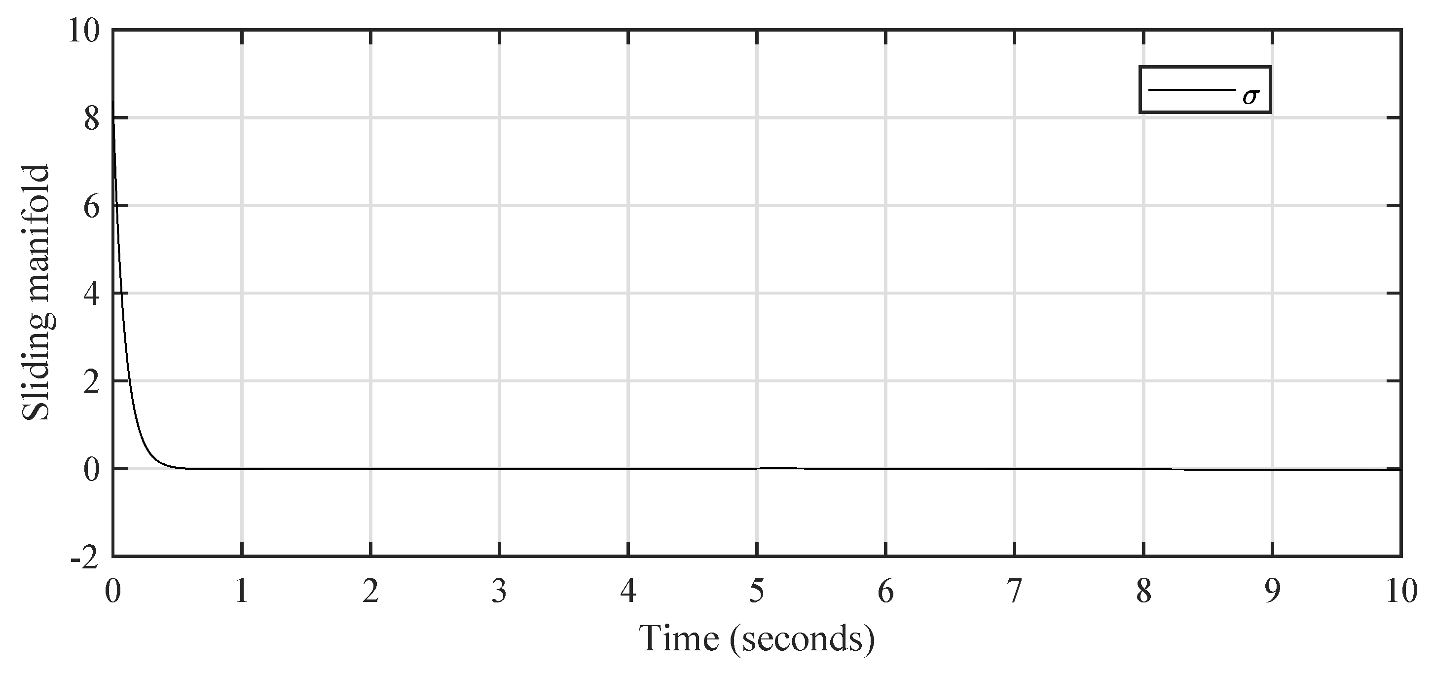
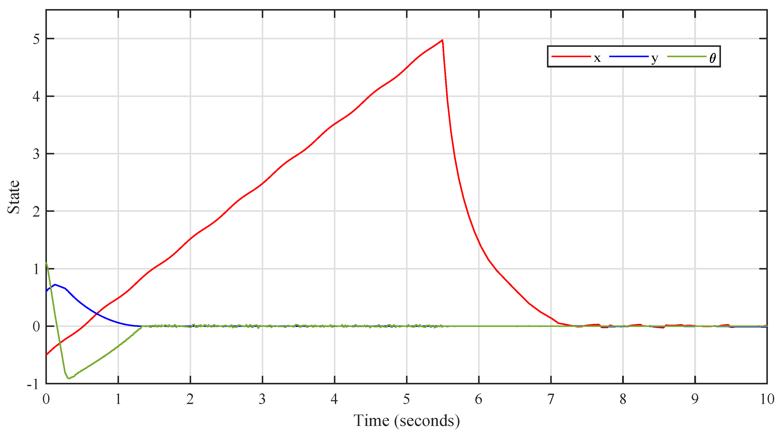
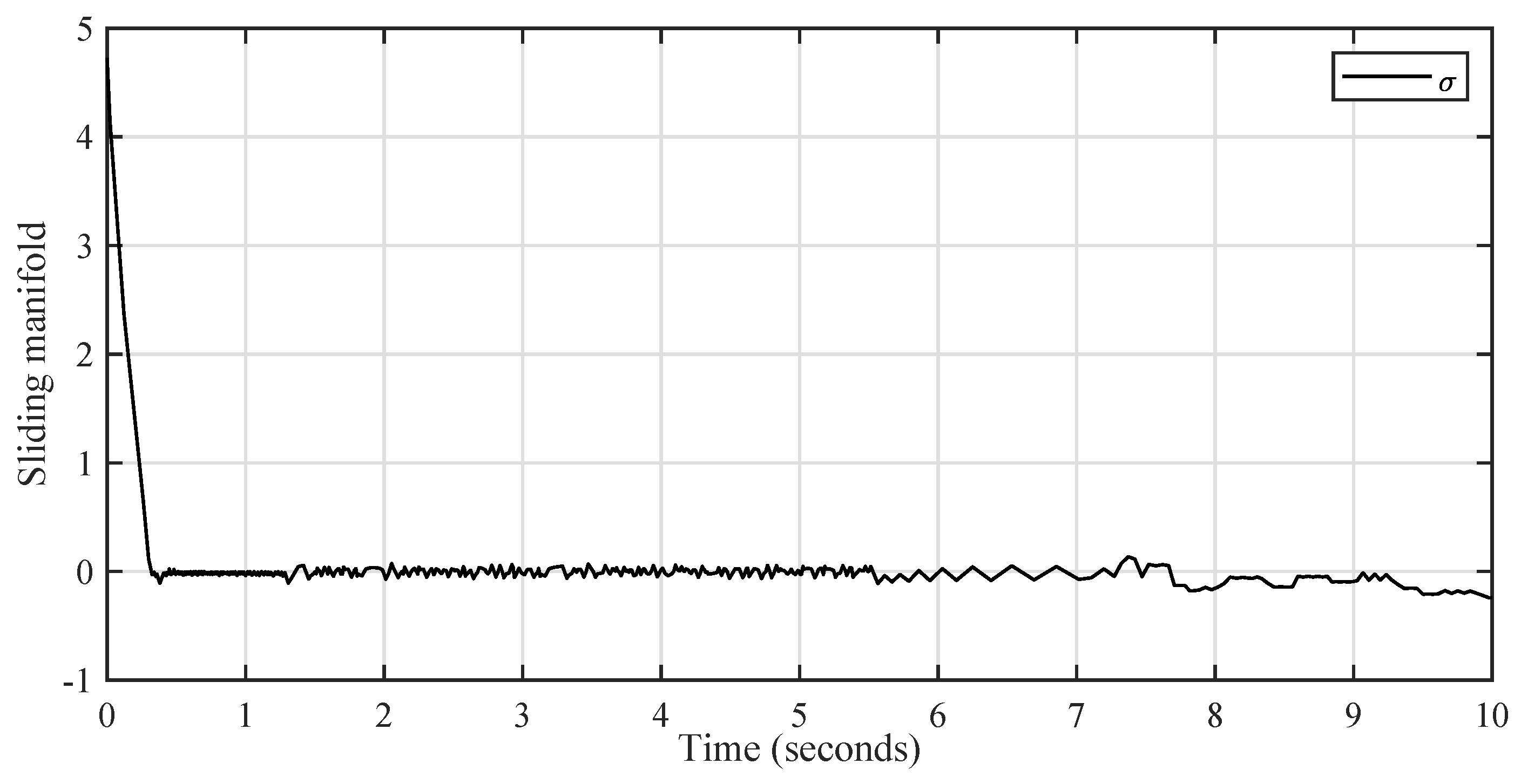
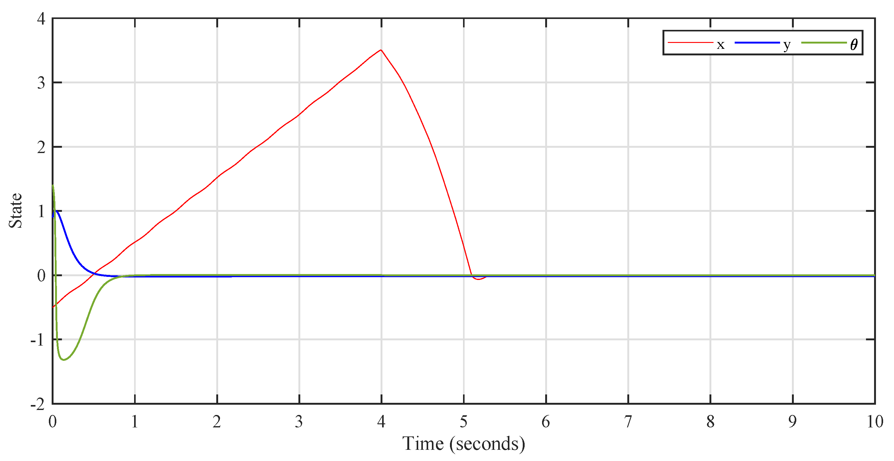
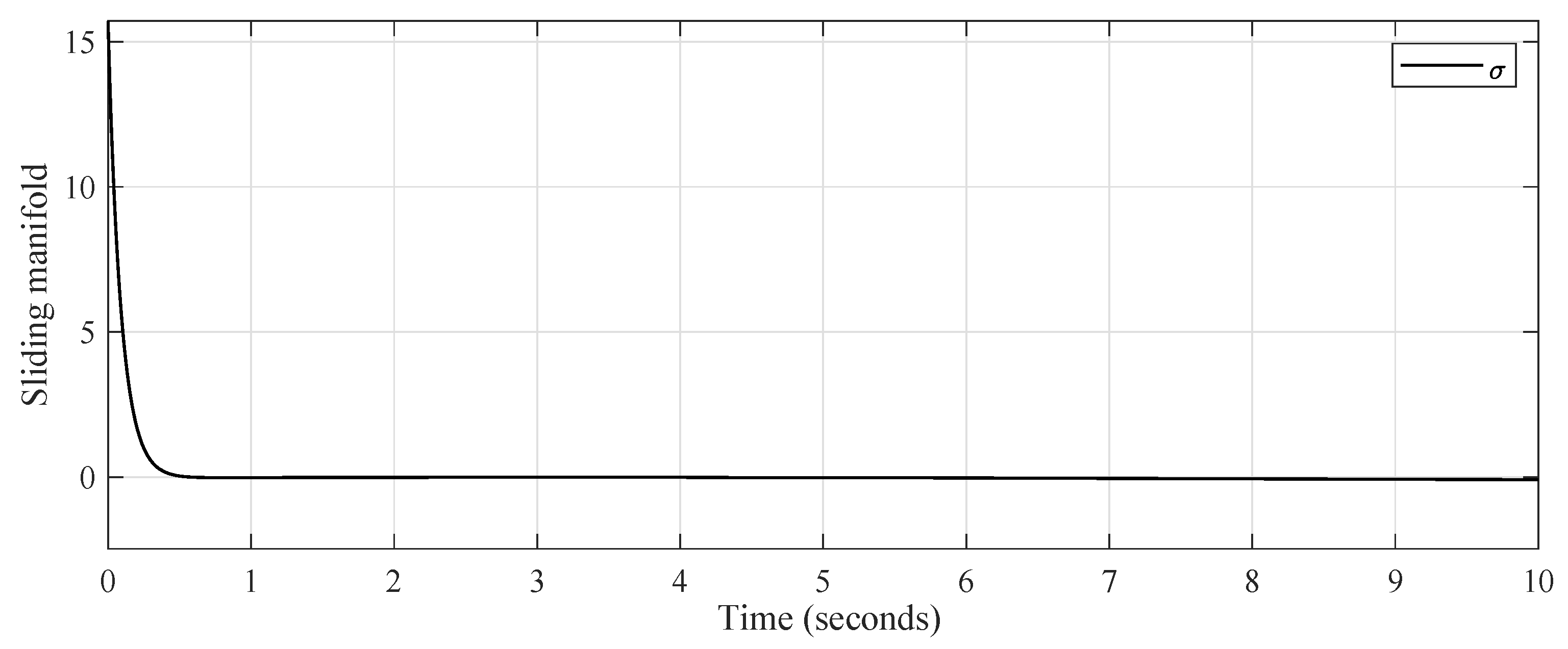
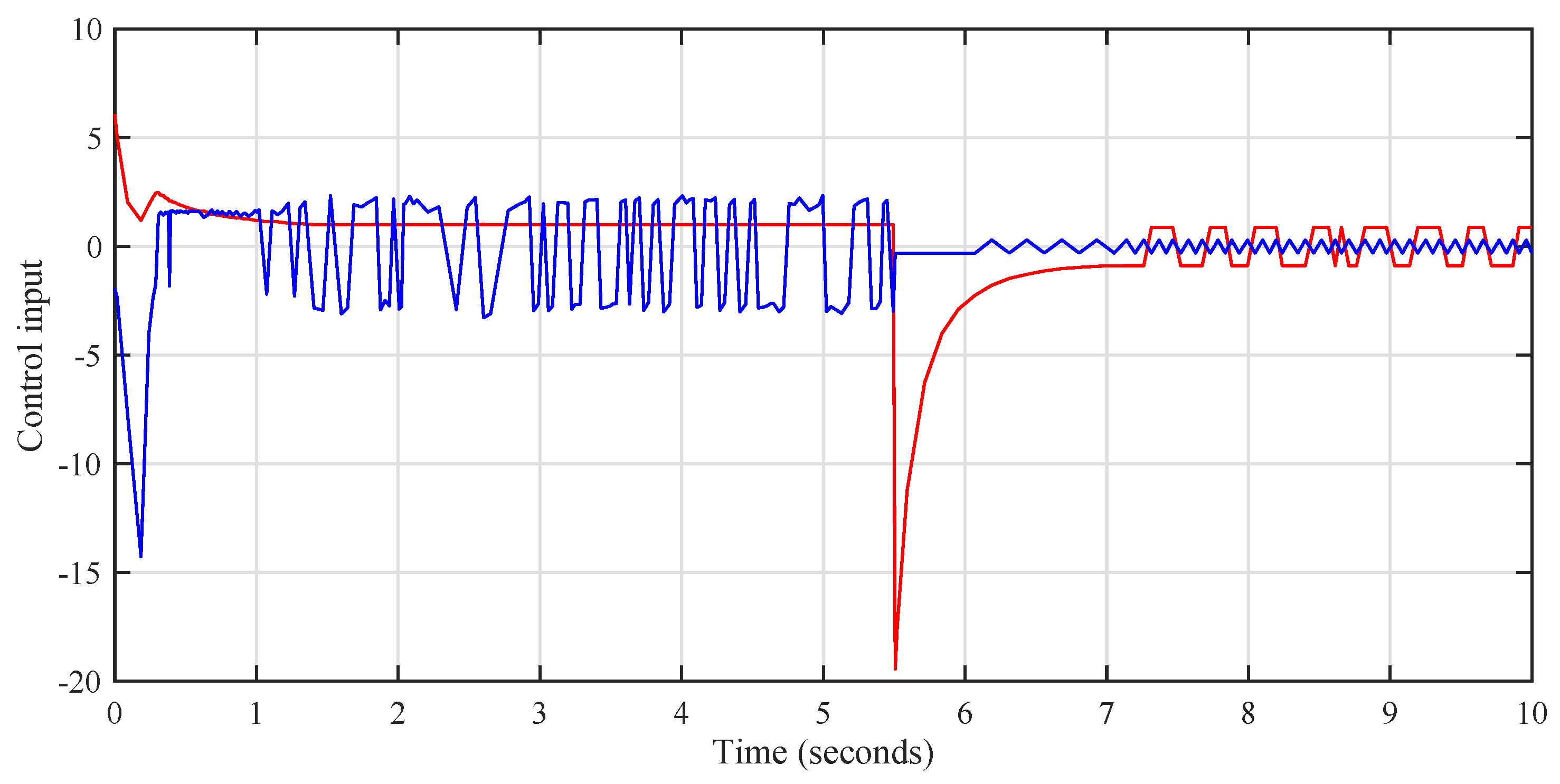
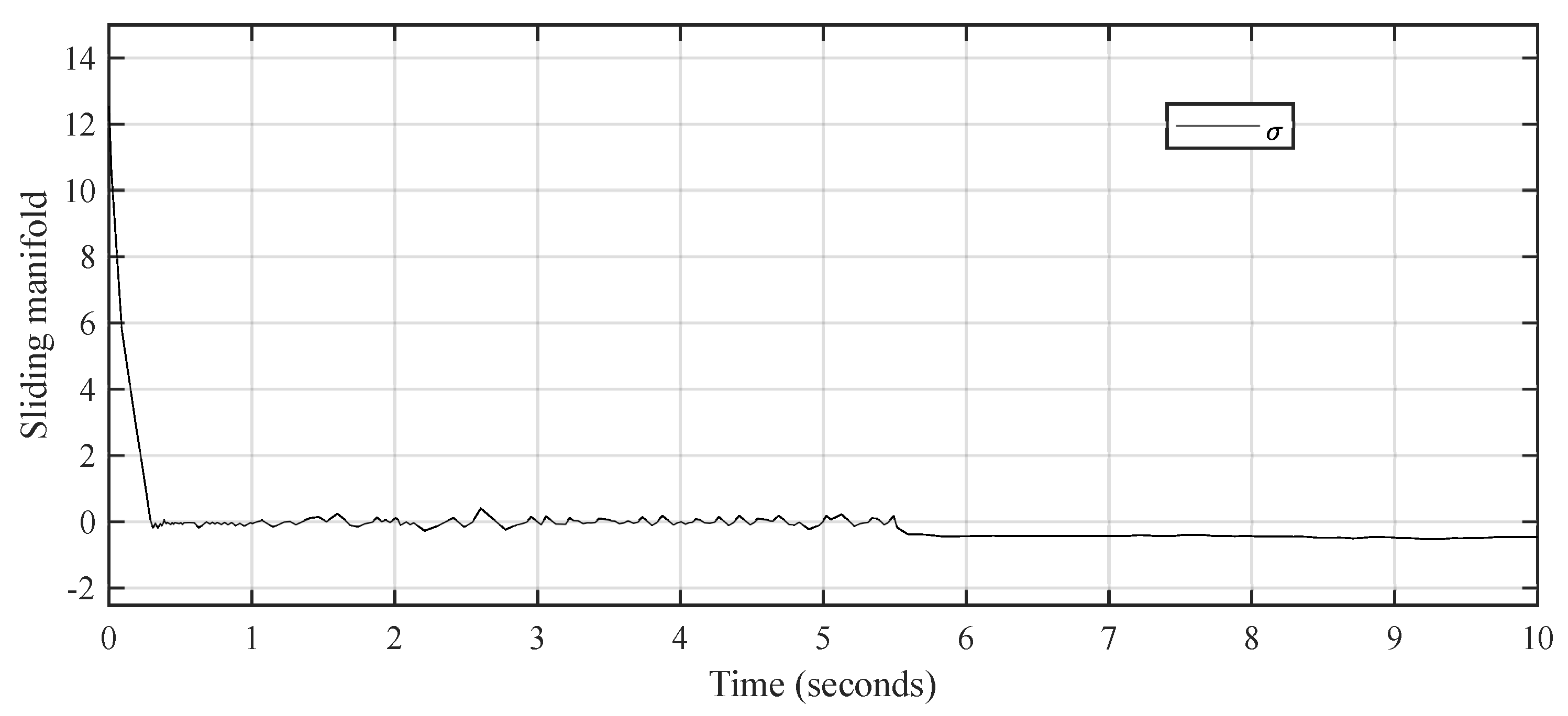
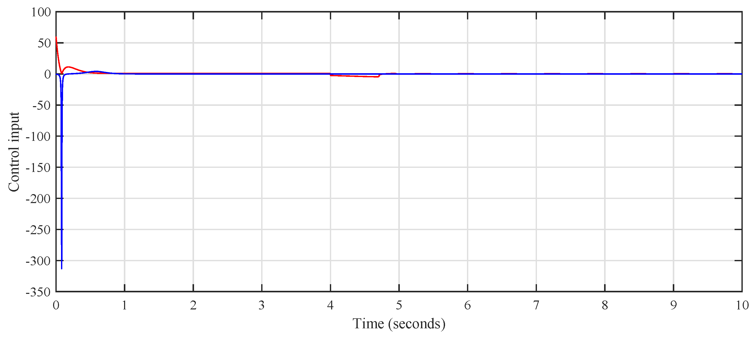
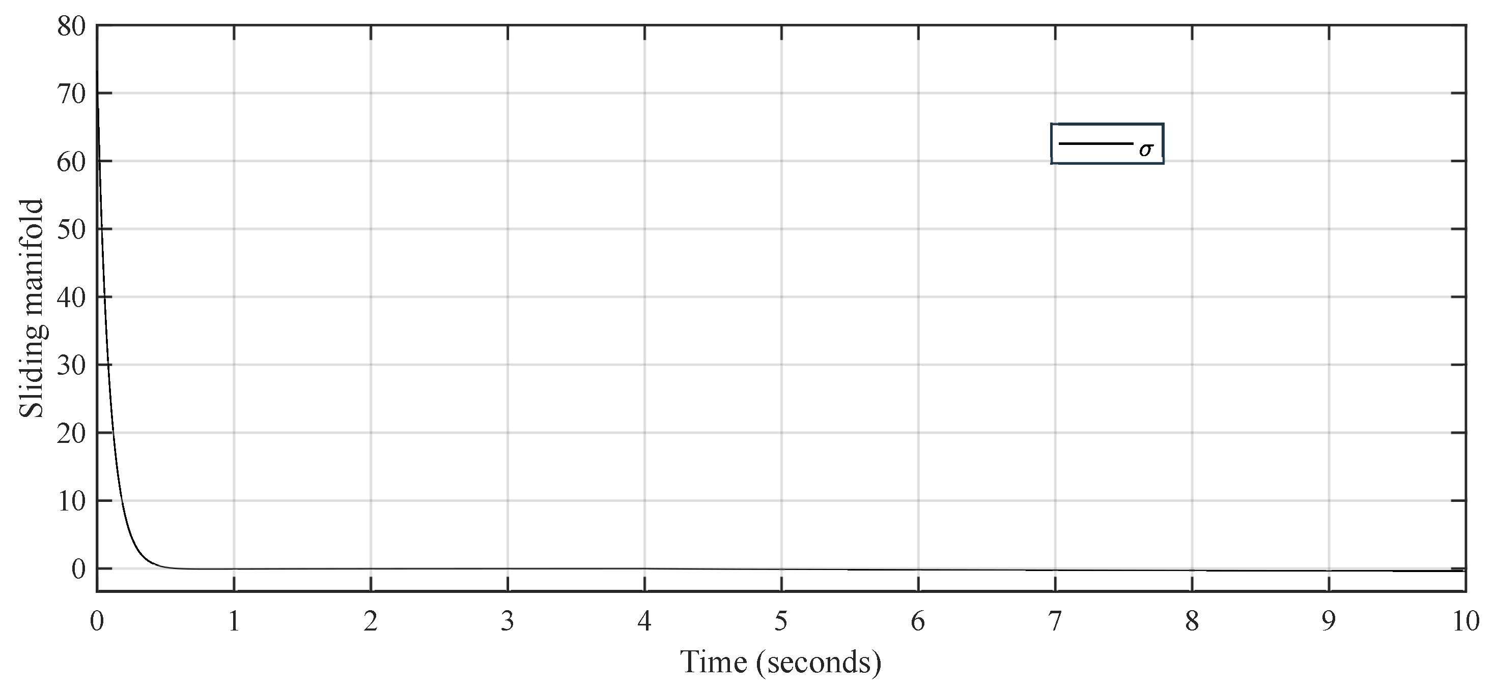
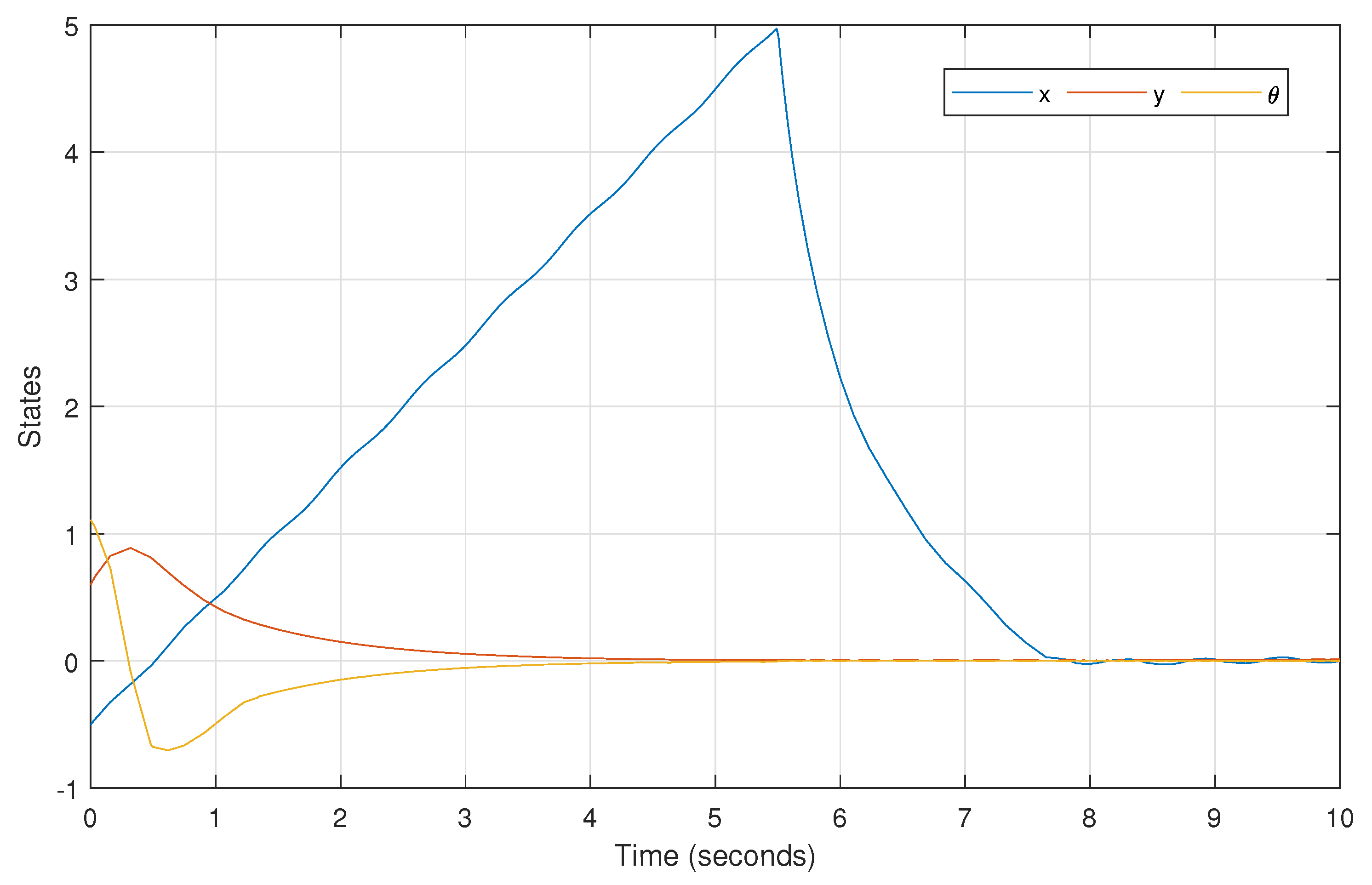
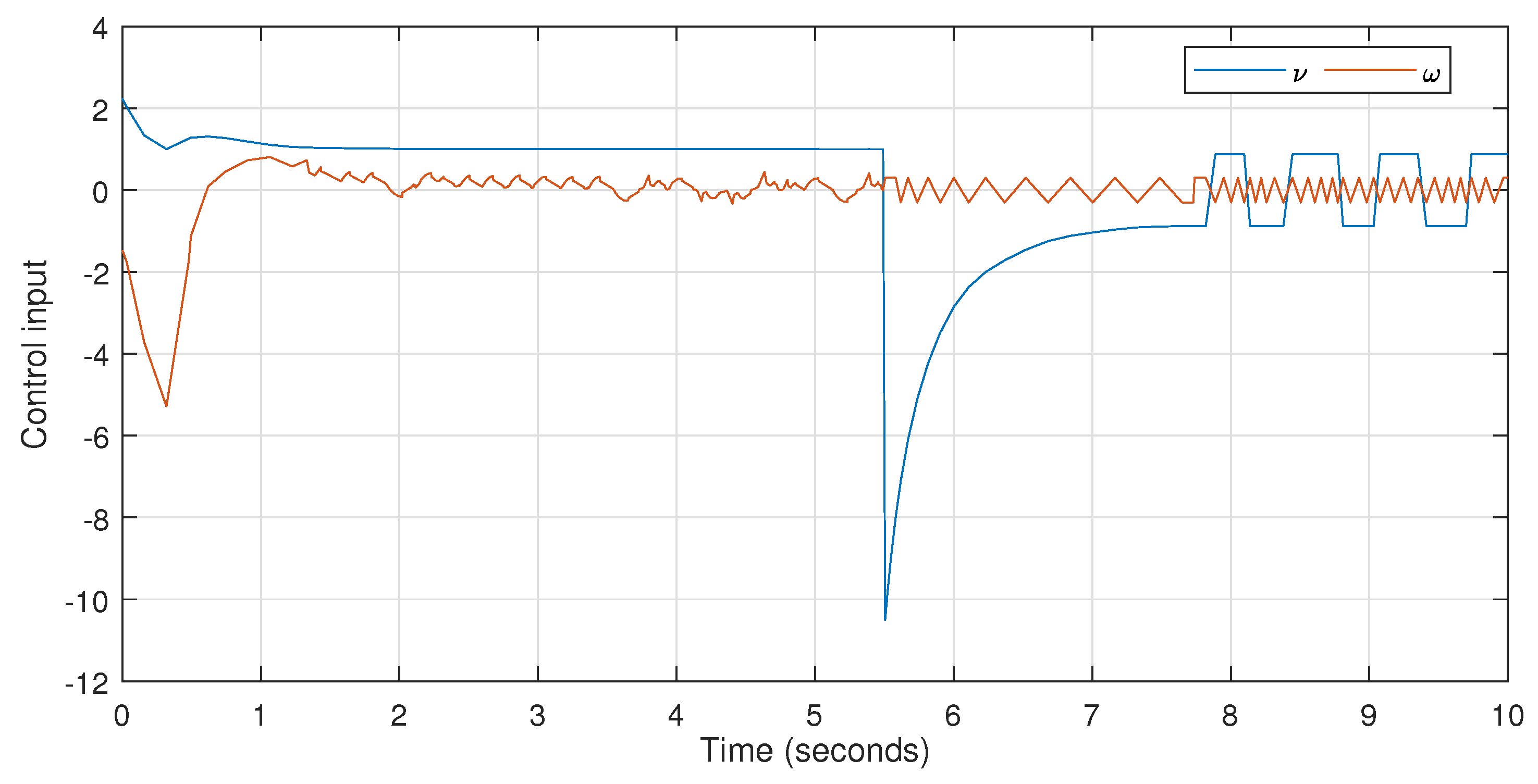
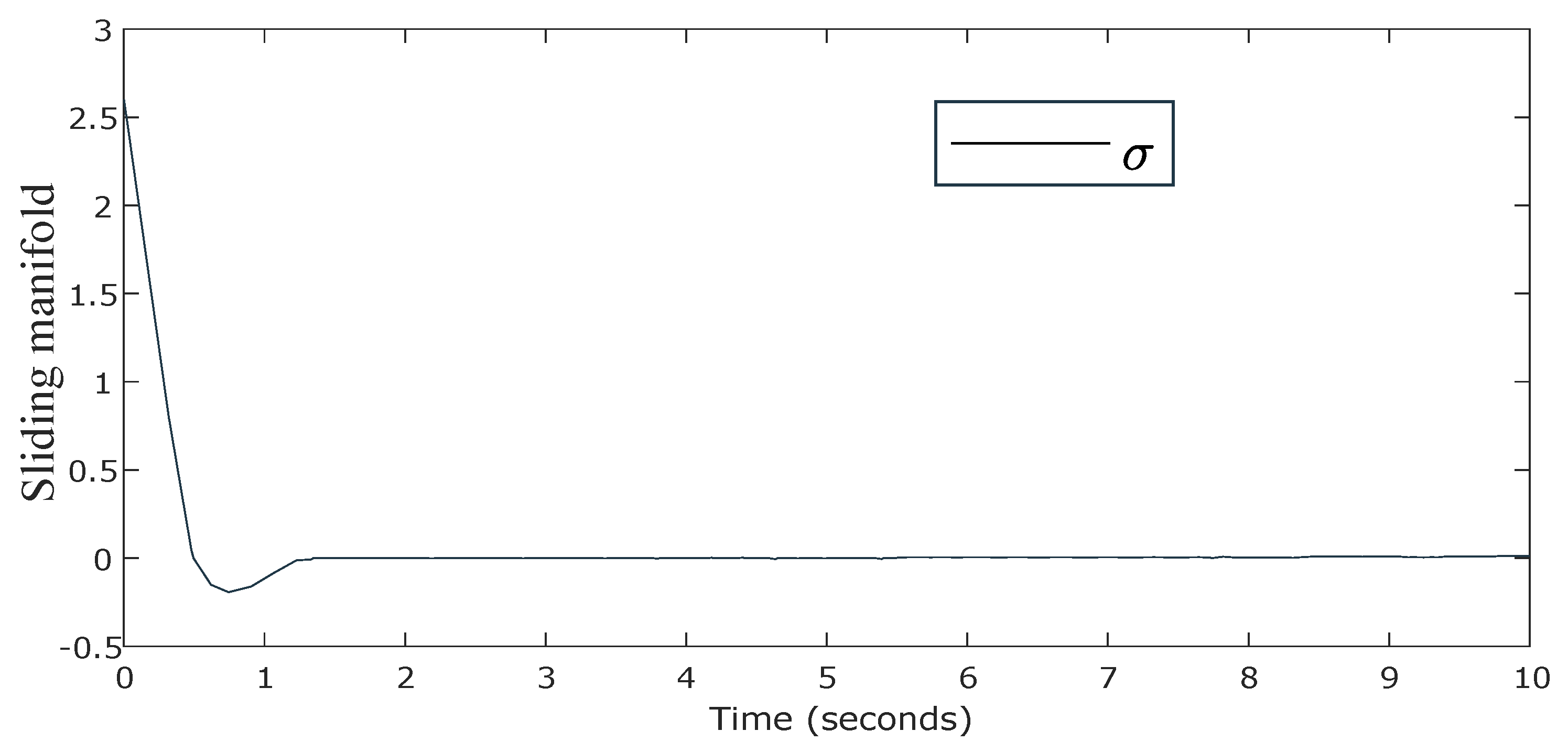
4. Analysis of Simulation Results

Numerical results are provided in this section to demonstrate the efficacy and application of the suggested control method. Consider that a robot with unicycle-like dynamics as given in (11) may be transformed into the system given in (13). A robot works as a system stabilizer (13) when it operates in a restricted context. The MR’s principal control aim is to solve the FnT stabilization problem.
We choose the simulations’ control parameters as ρ = 1 , α 1 = 1.2 , Ξ 0 = 0.3 , Ξ 1 = 0.78 , Ξ 2 = 1.3 , λ i = 0.2 , β = 1 , γ = 10 , κ = 0.99 , q = 0.6 , φ 1 = 10 , and φ 2 = 0.6 .
Equation (13) is a fixed-time stable system with a preset time T 1 = 4 s, notwithstanding the existence of disturbances, as a result of the FO switching control laws in Equations (45) and (46). Three scenarios are presented in the simulations to examine the efficacy of the suggested control method. The initial conditions are proposed as follows: (i) for the first scenario, ( ε 0 ( 0 ) , ε 1 ( 0 ) , ε 2 ( 0 ) ) = ( 0.5 , 0.6 , 2); (ii) for the second scenario, ( 0.5 , 0.9 , 6); and (iii) for the third scenario ( 0.7 , 1, 60).
Three distinct perturbations are chosen to further examine the performance of the fixed-time method utilizing FO-FxT-SCL and FxT-FO-GSMC:
( i ) d 0 = 0.2 cos ( 10 t ) d 1 = 0.4 cos ( 13 t )
( i i ) d 0 = 0.2 sin ( 17 t ) d 1 = 0.4 cos ( 14 t )
and
( i i i ) d 0 = 0.2 tanh ( 20 t 10 ) + 0.2 cos ( 10 t ) d 1 = 0.2 tanh ( 25 t 10 ) + 0.5 cos ( 15 t )
The simulation results using the proposed controller are plotted in in Figure 2, Figure 3 and Figure 4 for the first case. The suggested controller’s convergence time is about 5 s, which is virtually constant and significantly less than the intended length of 10 s as the starting value increases, as shown in Figure 2. In the first case, Figure 2 depicts the appropriate linear and angular velocities, whereas Figure 3 depicts the control inputs. The figures clearly indicate that the suggested control method stabilizes the MR outputs under perturbations in the fixed time T = 4 s, and that the control inputs are smooth and have lower magnitudes during transients. The sliding manifold, which converges to zero, is presented in Figure 4. This demonstrates that in the presence of disruptions, all states remain stable.
In order to show that the proposed control approach is superior, we used the fixed-time approach presented by Defoort et al. in [30] for comparison. The control system suggested in [30] was used as a representative example of existing FxT techniques. The simulated circumstances for the two controllers were set to be the same in order to make a fair comparison.
The controller in this situation is
τ 0 = 1 i f t T 1 c 0 | ε 0 | 2 s i g n ( ε 0 ) ( ζ 0 + c 1 ) s i g n ( ε 0 )
τ 1 = a 1 + 2 ζ 1 + 3 a 2 ε 2 2 s i g n ( σ ) s i g ( a 3 σ + a 4 s i g ( σ ) 3 ) 0.5 i f t T 1 γ i s i g n ( ε 2 ) e l s e
with the sliding variable σ = ε 2 + s i g ( s i g ( ε 2 ) 2 + b 1 ε 1 + b 2 s i g ( ε 1 ) 3 ) 0.5 .
In addition, c 0 = 0.78 , ζ 0 = 0.78 , c 1 = 0.1 , a 1 = 4.2 , a 2 = 4.2 , a 3 = 2.1 , a 4 = 2.1 , ζ 1 = 0.3 , b 1 = 4.2 , b 2 = 4.2 , and γ i = 0.3 .
Figure 5, Figure 6 and Figure 7 depict the appropriate results from [30]. It is apparent that in the study by Defoort et al., the convergence time is considerably overestimated. During transients, this also leads to a greater control magnitude. In addition, the control signals are not smooth. It is clear that the FO controllers proposed in this paper have better performance than the switching control method proposed in [30].
In the second case, the state variables are shown for the proposed controller in Figure 8, Figure 9 and Figure 10 and the controller in [30] in Figure 11, Figure 12 and Figure 13. We can observe from these results that, in the presence of external shocks, the position and rolling angle converge to their starting circumstances. We can observe from the results in Figure 9 that the control inputs are smooth and that the FO controller can reject unknown disturbances. In reality, this scenario is more realistic, and the FO control methods are primarily responsible for the MR’s stability and the sliding manifold converging to zero as shown in Figure 10.
In the last case, the state variables, control inputs, and sliding manifold are represented, respectively, in Figure 14, Figure 15 and Figure 16. Under perturbations, all state outputs converge to their initial conditions in a fixed time. The smooth and realizable amplitudes of the inputs, as shown in Figure 15, indicate that the MR is more stable in these circumstances.
To demonstrate that the suggested control strategy is preferable, we compared it to the high-order sliding mode control approach, as an example of an existing super-twisting approach used in the simulation in case 1. To establish a fair comparison, the simulated circumstances for the two controllers were configured to be the same. The controller in this situation is
τ 0 = 1 i f t T 1 c 0 | ε 0 | 2 s i g n ( ε 0 ) ( ζ 0 + c 1 ) s i g n ( ε 0 )
τ 1 = ϵ 2 4 | σ | 0.5 s i g n ( σ ) 2 s i g n ( σ ) d τ i f t T 1 γ i s i g n ( ε 2 ) e l s e
with the sliding variable σ = ε 1 + ε 2 . The results of this simulation are presented in Figure 17, Figure 18 and Figure 19.
The state variables are plotted in Figure 17. The difference between the proposed control and the super-twisting control is that the convergence time of the ST control algorithm increases slowly and is maintained below the prescribed time of 10 s as the initial values increase. In other words, regardless of the starting conditions, the proposed control algorithm ensures that the robot may be parked within the given time without violating the limitations. The ST method, on the other hand, has an excessively long convergence time. Furthermore, the advantages of the fixed-time FO control proposed in this paper over existing controls such as the super-twisting algorithm and the fixed-time control proposed by Defoort et al. [30] are that the proposed control provides higher accuracy and faster convergence due to the use of fractional operators in the concepts of sliding manifolds and control inputs.
Remark 4.
The suggested control method was compared to the fixed-time strategy mentioned in [30]. In addition, unlike in [27], where the state variables can only converge to zero asymptotically due to the use of sliding variables, the proposed control scheme, which uses fractional-order global sliding surface manifolds, can guarantee finite-time zero stability in the second system and fixed-time stability in the first system.

5. Conclusions

In this paper, two switching control approaches were designed for the first- and second-order systems of an MR under external disturbances. An original FO switching control law with D γ ( ε ) , 0 ε < 1 was suggested for the stabilization of the first-order systems of the MR. This controller was designed based on the FO sign function. Compared to an integer-order (IO) sign function, the proposed controller with an FO sign function can achieve faster convergence. To obtain FxT stability, the FO controller was combined with constant gain. In addition, an original FO global SMC was developed for the global stabilization the second-order system of the MR. This method used a specific sliding manifold to achieve a finite-time convergence of the state variables. It was demonstrated that the proposed controllers coped with external disturbances and provided FxT stability. Finally, the simulation results supported the anticipated convergence time constraint and showed that the proposed control strategy can accomplish stabilization of the MR and suppress the negative effect of disturbances.

Author Contributions

Conceptualization, M.L. and M.D.; methodology, M.L.; software, M.L.; validation, M.D., S.B., S.K.M. and A.B.; formal analysis, M.L.; investigation, S.B.; resources, S.B.; data curation, M.L.; writing—original draft preparation, M.L.; writing—review and editing, M.L. and M.D.; visualization, S.B. and A.B.; supervision, M.D.; project administration, S.B. and S.K.M.; funding acquisition, S.B. All authors have read and agreed to the published version of the manuscript.

Funding

This research was funded by Ministry of Education, Saudi Arabia for funding this research work through project number MoE-IF-G-20-09.

Institutional Review Board Statement

The study was conducted according to the guidelines of the Declaration of Helsinki and approved by the Institutional Review Board.

Data Availability Statement

No data were used to support this study.

Acknowledgments

The authors extend their appreciation to the Deputyship for Research and Innovation, Ministry of Education, Saudi Arabia for funding this research work through project number MoE-IF-G-20-09.

Conflicts of Interest

All authors declare no conflict of interest.

References

  1. Fragapane, G.; de Koster, R.; Sgarbossa, F.; Strandhagen, J.O. Planning and control of autonomous mobile robots for intralogistics: Literature review and research agenda. Eur. J. Oper. Res. 2021, 294, 405–426. [Google Scholar] [CrossRef]
  2. Zhu, A.; Pauwels, P.; De Vries, B. Smart component-oriented method of construction robot coordination for prefabricated housing. Autom. Constr. 2021, 129, 103778. [Google Scholar] [CrossRef]
  3. Lee, W.J.; Ill Kwag, S.; Ko, Y.D. Optimal capacity and operation design of a robot logistics system for the hotel industry. Tour. Manag. 2020, 76, 103971. [Google Scholar] [CrossRef]
  4. Gao, F.; Wu, Y.; Huang, J.; Liu, Y. Output feedback stabilization within prescribed finite time of asymmetric time-varying constrained nonholonomic systems. Int. J. Robust Nonlinear Control 2021, 31, 427–446. [Google Scholar] [CrossRef]
  5. Stolfi, A. Discontinuous control of nonholonomic systems. Syst. Control Lett. 1996, 27, 37–45. [Google Scholar] [CrossRef]
  6. Brockett, R.W. Asymptotic stability and feedback stabilization. Differ. Geom. Control. Theory 1983, 27, 181–191. [Google Scholar]
  7. Sánchez-Torres, J.D.; Defoort, M.; Muñoz-Vázquez, A.J. Predefined-time stabilisation of a class of nonholonomic systems. Int. J. Control 2020, 93, 2941–2948. [Google Scholar] [CrossRef]
  8. Huang, Y.; Su, J. Output feedback stabilization of uncertain nonholonomic systems with external disturbances via active disturbance rejection control. ISA Trans. 2020, 104, 245–254. [Google Scholar] [CrossRef]
  9. Ge, S.S.; Wang, Z.; Lee, T.H. Adaptive stabilization of uncertain nonholonomic systems by state and output feedback. Automatica 2003, 39, 1451–1460. [Google Scholar] [CrossRef]
  10. Wang, H.; Zhu, Q. Adaptive output feedback control of stochastic nonholonomic systems with nonlinear parameterization. Automatica 2018, 98, 247–255. [Google Scholar] [CrossRef]
  11. Liu, Z.G.; Wu, Y.Q.; Sun, Z.Y. Output feedback control for a class of high-order nonholonomic systems with complicated nonlinearity and time-varying delay. J. Frankl. Inst. 2017, 354, 4289–4310. [Google Scholar] [CrossRef]
  12. Jiang, Z.P. Robust exponential regulation of nonholonomic systems with uncertainties. Automatica 2000, 36, 189–209. [Google Scholar] [CrossRef]
  13. Tian, Y.P.; Li, S. Exponential stabilization of nonholonomic dynamic systems by smooth time-varying control. Automatica 2002, 38, 1139–1146. [Google Scholar] [CrossRef]
  14. Yu, J.; Zhao, Y. Global robust stabilization for nonholonomic systems with dynamic uncertainties. J. Frankl. Inst. 2020, 357, 1357–1377. [Google Scholar] [CrossRef]
  15. Gao, F.; Yuan, F. Adaptive finite-time stabilization for a class of uncertain high order nonholonomic systems. ISA Trans. 2015, 54, 75–82. [Google Scholar] [CrossRef]
  16. Gao, F.; Wu, Y.; Zhang, Z. Finite-time stabilization of uncertain nonholonomic systems in feedforward-like form by output feedback. ISA Trans. 2015, 59, 125–132. [Google Scholar] [CrossRef]
  17. Gao, F.; Yuan, Y.; Wu, Y. Finite-time stabilization for a class of nonholonomic feedforward systems subject to inputs saturation. ISA Trans. 2016, 64, 193–201. [Google Scholar] [CrossRef]
  18. Chen, X.; Zhang, X.; Zhang, C.; Chang, L. A time-varying high-gain approach to feedback regulation of uncertain time-varying nonholonomic systems. ISA Trans. 2020, 98, 110–122. [Google Scholar] [CrossRef]
  19. Wu, D.; Cheng, Y.; Du, H.; Zhu, W.; Zhu, M. Finite-time output feedback tracking control for a nonholonomic wheeled mobile robot. Aerosp. Sci. Technol. 2018, 78, 574–579. [Google Scholar] [CrossRef]
  20. Gao, F.; Huang, J.; Zhu, X.; Wu, Y. Output feedback stabilization via nonlinear mapping for time-varying constrained nonholonomic systems in prescribed finite time. Inf. Sci. (NY) 2021, 550, 297–312. [Google Scholar] [CrossRef]
  21. Gao, F.; Huang, J.; Shi, X.; Zhu, X. Nonlinear mapping-based fixed-time stabilization of uncertain nonholonomic systems with time-varying state constraints. J. Frankl. Inst. 2020, 357, 6653–6670. [Google Scholar] [CrossRef]
  22. Guo, Y.; Ma, B.L. Global sliding mode with fractional operators and application to control robot manipulators. Int. J. Control 2019, 92, 1497–1510. [Google Scholar] [CrossRef]
  23. Labbadi, M.; Boukal, Y.; Cherkaoui, M.; Djemai, M. Fractional-order global sliding mode controller for an uncertain quadrotor UAVs subjected to external disturbances. J. Frankl. Inst. 2021, 358, 4822–4847. [Google Scholar] [CrossRef]
  24. Nojavanzadeh, D.; Badamchizadeh, M. Adaptive fractional-order non-singular fast terminal sliding mode control for robot manipulators. IET Control Theory Appl. 2016, 10, 1565–1572. [Google Scholar] [CrossRef]
  25. Aghababa, M.P. A fractional sliding mode for finite-time control scheme with application to stabilization of electrostatic and electromechanical transducers. Appl. Math. Model. 2015, 39, 6103–6113. [Google Scholar] [CrossRef]
  26. Labbadi, M.; Boukal, Y.; Taleb, M.; Cherkaoui, M. Fractional order sliding mode control for the tracking problem of Quadrotor UAV under external disturbances. In Proceedings of the 2020 European Control Conference (ECC), St. Petersburg, Russia, 12–15 May 2020; pp. 1595–1600. [Google Scholar]
  27. Labbadi, M.; Boukal, Y.; Cherkaoui, M. Path Following Control of Quadrotor UAV With Continuous Fractional-Order Super Twisting Sliding Mode. J. Intell. Robot. Syst. Theory Appl. 2020, 100, 1429–1451. [Google Scholar] [CrossRef]
  28. Labbadi, M.; Nassiri, S.; Bousselamti, L.; Bahij, M.; Cherkaoui, M. Fractional-order fast terminal sliding mode control of uncertain quadrotor UAV with time-varying disturbances. In Proceedings of the 2019 8th International Conference on Systems and Control (ICSC 2019), Marrakesh, Morocco, 23–25 October 2019. [Google Scholar]
  29. Labbadi, M.; El Moussaoui, H. An improved adaptive fractional-order fast integral terminal sliding mode control for distributed quadrotor. Math. Comput. Simul. 2021, 188, 120–134. [Google Scholar] [CrossRef]
  30. Defoort, M.; Demesure, G.; Uo, Z.; Zuo, Z.; Polyakov, A.; Djemai, M. Fixed-time stabilisation and consensus of non-holonomic systems. IET Control Theory Appl. 2016, 10, 2497–2505. [Google Scholar] [CrossRef]
  31. Podlubny, I. Fractional Differential Equations; Academic: New York, NY, USA, 1999. [Google Scholar]
  32. Das, S. Functional Fractional Calculus for System Identification and Controls; Springer: Berlin/Heidelberg, Germany, 2008. [Google Scholar]
  33. Podlubny, I. Geometric and physical interpretation of fractional integration and fractional differentiation. Fract. Calc. Appl. Anal. 2002, 5, 367–386. [Google Scholar]
  34. Polyakov, A. Nonlinear feedback design for fixed-time stabilization of linear control systems. IEEE Trans. Autom. Control 2012, 57, 2106–2110. [Google Scholar] [CrossRef] [Green Version]
  35. Bhat, S.; Bernstein, D. Geometric homogeneity with applications to finite time stability. Math. Control Signals Syst. 2005, 17, 101–127. [Google Scholar] [CrossRef] [Green Version]
  36. Yu, S.; Yu, X.; Stonier, R. Continuous finite-time control for robotic manipulators with terminal sliding modes. In Proceedings of the Sixth International Conference of Information Fusion, Cairns, QLD, Australia, 8–11 July 2003; pp. 1433–1440. [Google Scholar]
  37. Moulay, E.; Perruquetti, W. Finite time stability and stabilization of a class of continuous systems. J. Math. Anal. Appl. 2006, 323, 1430–1443. [Google Scholar] [CrossRef] [Green Version]
  38. Yin, C.; Chen, Y.; Zhong, S.M. Fractional-order sliding mode based extremum seeking control of a class of nonlinear systems. Automatica 2014, 50, 3173–3181. [Google Scholar] [CrossRef]
Figure 1. The planar graph of a mobile robot.
Fractalfract 06 00177 g001
Figure 2. State trajectory graphs corresponding to the proposed FO-FxT-SCL and FxT-FO-GSMC in case 1.
Fractalfract 06 00177 g002
Figure 3. Control inputs obtained by the proposed FO-FxT-SCL and FxT-FO-GSMC in case 1.
Fractalfract 06 00177 g003
Figure 4. Evolution of the sliding manifold using the proposed FO-FxT-SCL and FxT-FO-GSMC in case 1.
Fractalfract 06 00177 g004
Figure 5. State trajectory graphs corresponding to the controller from [30] in case 1.
Fractalfract 06 00177 g005
Figure 6. Control inputs obtained by the controller from [30] in case 1.
Fractalfract 06 00177 g006
Figure 7. Evolution of the sliding manifold using the controller from [30] in case 1.
Fractalfract 06 00177 g007
Figure 8. State trajectory graphs corresponding to the proposed FO-FxT-SCL and FxT-FO-GSMC in case 2.
Fractalfract 06 00177 g008
Figure 9. Control inputs obtained by the proposed FO-FxT-SCL and FxT-FO-GSMC in case 2.
Fractalfract 06 00177 g009
Figure 10. Evolution of the sliding manifold using the proposed FO-FxT-SCL and FxT-FO-GSMC in case 2.
Fractalfract 06 00177 g010
Figure 11. State trajectory graphs corresponding to the controller from [30] in case 2.
Fractalfract 06 00177 g011
Figure 12. Control inputs obtained by the controller from [30] in case 2.
Fractalfract 06 00177 g012
Figure 13. Evolution of the sliding manifold using the controller from [30] in case 2.
Fractalfract 06 00177 g013
Figure 14. State trajectory graphs corresponding to the proposed FO-FxT-SCL and FxT-FO-GSMC in case 3.
Fractalfract 06 00177 g014
Figure 15. Control inputs obtained by the proposed FO-FxT-SCL and FxT-FO-GSMC in case 3.
Fractalfract 06 00177 g015
Figure 16. Evolution of the sliding manifold using the proposed FO-FxT-SCL and FxT-FO-GSMC in case 3.
Fractalfract 06 00177 g016
Figure 17. State trajectory graphs corresponding to the super-twisting control in case 1.
Fractalfract 06 00177 g017
Figure 18. Control inputs obtained by the super-twisting control in case 1.
Fractalfract 06 00177 g018
Figure 19. Evolution of the sliding manifold using the super-twisting control in case 1.
Fractalfract 06 00177 g019
Publisher’s Note: MDPI stays neutral with regard to jurisdictional claims in published maps and institutional affiliations.

