Article

Electronically Controlled Power-Law Filters Realizations

by
Errikos Tsouvalas
1,
Stavroula Kapoulea
1,
Costas Psychalinos
1,*,
Ahmed S. Elwakil
2,3,4 and
Dražen Jurišić
5
1
Department of Physics, Electronics Laboratory, University of Patras, GR-26504 Rio Patras, Greece
2
Department of Electrical and Computer Engineering, University of Sharjah, Sharjah P.O. Box 27272, United Arab Emirates
3
Nanoelectronics Integrated Systems Center (NISC), Nile University, Giza 12677, Egypt
4
Department of Electrical and Software Engineering, University of Calgary, Calgary, AB T2N 1N4, Canada
5
Faculty of Electrical Engineering and Computing, University of Zagreb, HR-10000 Zagreb, Croatia
*
Author to whom correspondence should be addressed.
Fractal Fract. 2022, 6(2), 111; https://doi.org/10.3390/fractalfract6020111
Submission received: 12 January 2022 / Revised: 31 January 2022 / Accepted: 11 February 2022 / Published: 14 February 2022
(This article belongs to the Special Issue 2021 Feature Papers by Fractal Fract's Editorial Board Members)

Abstract

:
A generalized structure that is capable of implementing power-law filters derived from 1st and 2nd-order mother filter functions is presented in this work. This is achieved thanks to the employment of Operational Transconductance Amplifiers (OTAs) as active elements, because of the electronic tuning capability of their transconductance parameter. Appropriate design examples are provided and the performance of the introduced structure is evaluated through simulation results using the Cadence Integrated Circuits (IC) design suite and Metal Oxide Semiconductor (MOS) transistors models available from the Austria Mikro Systeme (AMS) 0.35 μ m Complementary Metal Oxide Semiconductor (CMOS) process.

1. Introduction

The replacement of the Laplacian operator by its fractional-order counterpart (i.e., s s α , where 0 < α < 1 ) has been broadly utilized for transposing integer-order transfer functions into the fractional-order domain [1]. Therefore, the rational approximation of the resulted fractional-order filter functions has gained a significant research interest [2,3,4,5,6].
The power-law filters constitute an alternative way for deriving fractional-order transfer functions, without employing the approximation of the fractional-order Laplacian operator. In particular, power-law filters are based on the employment of transfer functions, which are derived from their integer-order counterparts, raised to a non-integer exponent [7]. Accordingly, starting from an integer-order transfer function H m ( s ) , which will be denoted as the mother function hereinafter, the resulting power-law transfer function can be expressed by (1):
H ( s ) = H m ( s ) α ,
where the magnitude and phase responses are related to those of the mother function as:
| H ( ω ) | = H m ( ω ) α ,
H ( ω ) = α · H m ( ω ) ,
The insertion of the non-integer exponent α offers an additional degree of freedom, that allows precise adjustment of the filter’s characteristics, including the cutoff frequency and the slope of the transition from the passband to stopband. In particular, the derived frequency responses exhibit an attenuation gradient scaled by a factor equal to the order of the filter, compared to the corresponding response of the mother filter function [8,9,10].
The approximation of the power-law filter function H ( s ) can be conducted in the following way: the frequency responses of (2a) and (2b) are initially obtained, and, afterward, they are approximated through appropriate magnitude and phase curve-fitting-based techniques [11,12]. The obtained functions have the form of rational integer-order transfer functions, which can be realized using multi-feedback structures, cascade connection, or sum of the intermediate filter functions. This has been followed in [7], where the Sanathanan–Koerner (SK) least-square iterative method has been employed for performing the curve-fitting approximation of both magnitude and phase frequency responses and the derived integer-order rational transfer functions have been realized by an operational amplifier (op-amp)-based Follow-the-Leader Feedback (FLF) structure. In [13], an optimization of power-law filter functions is performed for three different objective functions and 2nd-order mother filter functions. The presented implementation is based on the employment of Current-Feedback Operational Amplifiers (CFOAs) as active elements accompanied by resistors and capacitors.
The above implementations suffer from the absence of the adjustability of the filter characteristics, in the sense that the resistors and capacitors must be substituted by other ones with different values for each type and order of the desirable transfer function.
To overcome this obstacle, a novel configuration is presented in this work, where OTAs have been employed as active elements for implementing the required integration stages in the Inverse Follow-the-Leader Feedback (IFLF) structure, which implements the integer-order rational transfer functions derived through the utilization of the SK curve-fitting-based method. Owing to the small-signal nature of the transconductance parameter of the OTAs, the time constants of the integration stages, as well as the scaling factors of the summation stages, become electronically adjustable, making the structure versatile with regards to the implementation of power-law filters. The idea of electronic tuning using OTA-C structures with IFLF configuration is not new, it has been successfully applied in fractional-order filter design [14].
The paper is organized as follows: a brief description of the behavior of power-law filters is given in Section 2, while their approximation is discussed in Section 3. The proposed implementation is presented in Section 4, while the derived post-layout simulation results are presented in Section 5.

2. Power-Law Filters

2.1. Power-Law Filters Derived from 1st-Order Mother Functions

The transfer function of a power-law Low-Pass (LP) filter, derived from a 1st-order mother function with pole ω 0 , is given by:
H L P ( s ) = ω 0 s + ω 0 α ,
with 0 < α < 1 being the order of the filter. Substituting variable s with j ω , the derived expressions of the magnitude and phase frequency responses are given by the following expressions:
H L P ( ω ) = 1 1 + ω ω 0 2 α / 2 ,
H L P ( ω ) = α · tan 1 ω ω 0 .
Using (4a) and (4b), the half-power frequency and the phase at this frequency are calculated by the formulas in (5a) and (5b), respectively.
ω h , L P = ω 0 · 2 1 / α 1 ,
H L P ( ω h , L P ) = α · tan 1 2 1 / α 1 .
The corresponding expressions of a high-pass (HP) filter are given by (6)–(8b).
H H P ( s ) = s s + ω 0 α
H H P ( ω ) = ω ω 0 α ω ω 0 2 + 1 α / 2
H H P ( ω ) = α · π 2 tan 1 ω ω 0 .
ω h , H P = ω 0 2 1 / α 1
H H P ( ω h , H P ) = α · π 2 tan 1 1 2 1 / α 1 .
The slope of the stopband attenuation for these types of power-law filters is 20 · α dB/dec; they also have the same pole frequency ω 0 . Considering (5a) and (8a), it is derived that the half-power frequencies of the low-pass and high-pass filters are located in equal logarithmic distance around the pole frequency, i.e., ω h , L P · ω h , H P = ω 0 [7].
From the expressions in (9) and (8a), it is obvious that the half-power frequency is not equal to the pole frequency. More specifically, ω h , L P > ω 0 and ω h , H P < ω 0 and exact location depends on the order of the filter. This situation is similar to that observed in the case of fractional-order filters, where the corresponding expressions are the following:
ω h , F O , L P / H P = ω 0 · 1 + cos 2 α π 2 cos α π 2 1 / α ,
The main difference is that in fractional-order filters the opposite conditions are valid: ω h , F O , L P < ω 0 and ω h , F O , H P > ω 0 , making power-law filters more preferable in the case that the cutoff frequency of the low-pass filter must be greater than the pole frequency or the cutoff frequency of the high-pass filter must be smaller than the pole frequency.
It must be mentioned at this point that for 1 < α < 2 the locations of the half-power frequencies with regards to the pole frequency are interchanged for the low and high-pass filters and this is easily derived by analyzing the transfer functions in (3) or (6) as products of a power-law term of order ( 1 α ) and an integer-order term.

2.2. Power-Law Filters Derived from 2nd-Order Mother Functions

Let us consider as mother function a 2nd-order LP filter function, then its power-law filter counterpart will be described by:
H L P ( s ) = ω 0 2 s 2 + ω 0 Q · s + ω 0 2 α ,
with ω 0 and Q being the pole frequency and the quality factor, respectively.
The magnitude and phase responses are given by:
H L P ( ω ) = 1 1 + ω ω 0 4 + ω ω 0 2 · 1 Q 2 2 α / 2 ,
H L P ( ω ) = α · tan 1 ω ω 0 · 1 Q 1 ω ω 0 2 .
The corresponding expressions in the case of an HP filter derived from a 2nd-order mother function are given by:
H H P ( s ) = s 2 s 2 + ω 0 Q · s + ω 0 2 α ,
H H P ( ω ) = ω ω 0 2 α 1 + ω ω 0 4 + ω ω 0 2 · 1 Q 2 2 α / 2 ,
H H P ( ω ) = α · π tan 1 ω ω 0 · 1 Q 1 ω ω 0 2 .
The slope of the stopband attenuation for these types of power-law filters is 40 · α dB / dec , while their cutoff frequencies, calculated considering a 3 dB drop from the maximum value of the gain in (11a) and (13a), respectively, are also located at symmetrical positions around the pole frequency.
In the case of a 2nd-order band-pass (BP) mother filter function, the derived expressions of the transfer function, as well as of frequency responses, are described by:
H B P ( s ) = ω 0 Q · s s 2 + ω 0 Q · s + ω 0 2 α ,
H B P ( ω ) = 1 Q α · ω ω 0 α 1 + ω ω 0 4 + ω ω 0 2 · 1 Q 2 2 α / 2 ,
H B P ( ω ) = α · π 2 tan 1 ω ω 0 · 1 Q 1 ω ω 0 2 .
For a band-stop (BS) mother filter, the corresponding expressions are provided by:
H B S ( s ) = s 2 + ω 0 2 s 2 + ω 0 Q · s + ω 0 2 α ,
H B S ( ω ) = 1 ω ω 0 2 α 1 + ω ω 0 4 + ω ω 0 2 · 1 Q 2 2 α / 2 ,
H B S ( ω ) = α · tan 1 ω ω 0 · 1 Q 1 ω ω 0 2 .
In both BP and BS power-law filters, the peak frequency is equal to the pole frequency, i.e., ω p e a k = ω 0 , independent from the order of the filter. The last one controls only the slopes of the transition bands, as they are given by the formula 40 · α dB / dec . This affects the lower ( ω h , l ) and upper ( ω h , u ) half-power frequencies, which are still located in symmetrical locations around the peak frequency. From all the above, it is obvious that the bandwidth of the filter can be adjusted through the order without disturbing the peak frequency and the maximum gain of the filter. In the case of the fractional-order filters, changes of the order affect both peak frequency and the maximum gain of the filter. Consequently, only power-law filters offer orthogonal dependence between the quality factor and the other filter characteristics (i.e., peak frequency and maximum gain) [7,15].

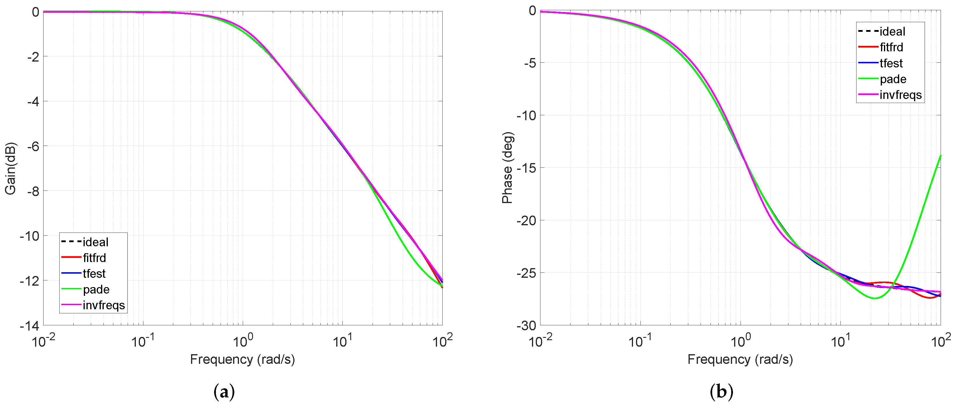
3. Approximation of Power-Law Filters’ Functions

The transfer functions of the previous section cannot be directly implemented, due to the non-integer power ( α ) that appears in both numerator and denominator. Conventional approximation methods, such as Oustaloup, Matsuda, or Continued Fraction Expansion are not suitable in the current problem, since these tools are able to approach the fractional-order Laplace operator s α [16,17,18,19,20]. Therefore, the following general methods will be considered: (a) curve fitting of the power-law function frequency response data, and (b) asymptotic of the power-law function using the Padé approximation tool.
The curve-fitting-based methods perform transfer-function estimation and are based on the following steps [7,11,12]:
(a)
Obtain the frequency-response data of the mother function within the desired frequency range using MATLAB freqresp function, then raise the obtained response to the power α for deriving the final response,
(b)
Obtain the data of the final response using the MATLAB function frd,
(c)
Choose the desired value of the approximation order (which will be the order of the derived approximate integer-order transfer function).
At this point, three options are available:
(a)
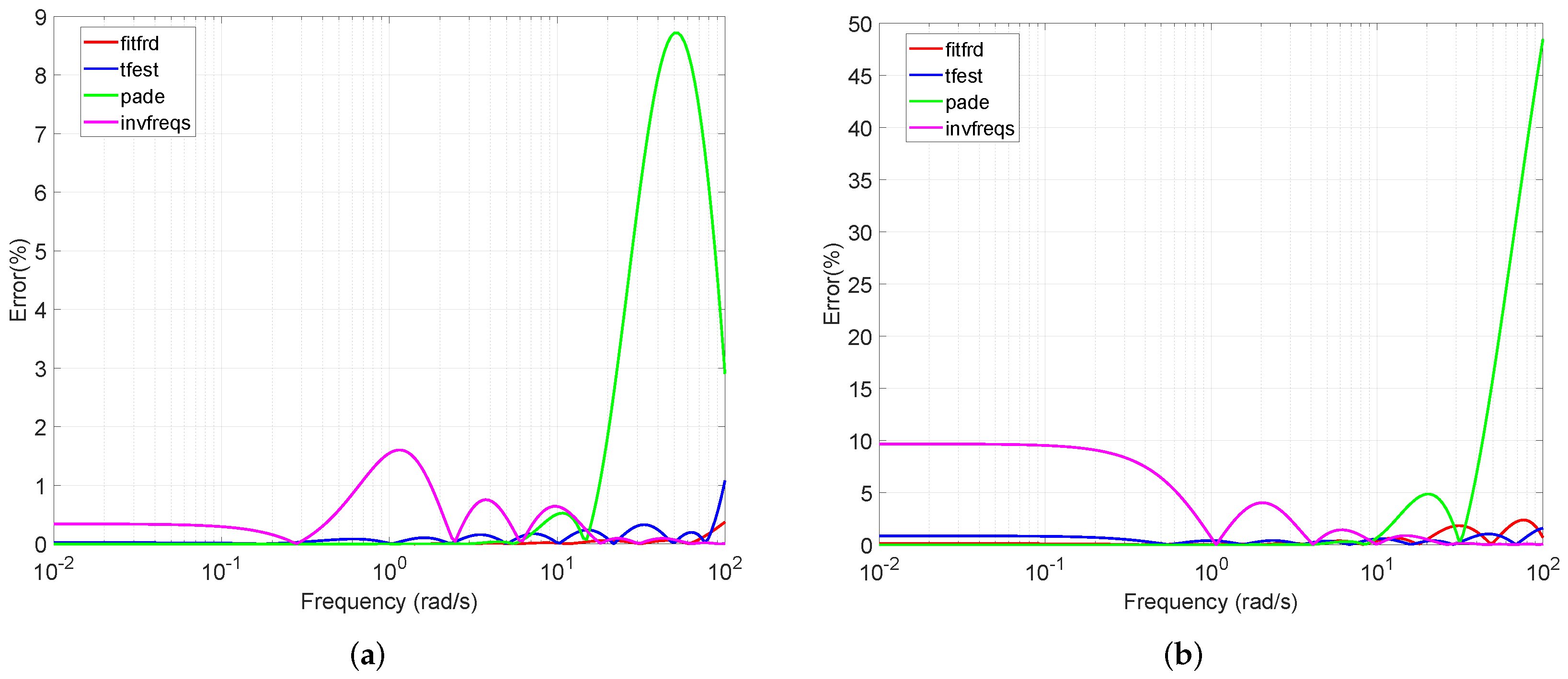
to obtain the state-space model of the data using the command fitfrd, which is based on the Sanathanan–Koerner (SK) least square iterative method, and then to convert this model to a transfer function using the command ss2tf,
(b)
to directly obtain the transfer-function model of the data, using the tfest function,
(c)
to directly obtain the transfer-function model of the data, using the invfreqs function.
Meanwhile, the Padé approximation method is actually a generalization of the asymptotic Taylor expansion, and is able to extract the information from power series expansions with only a few known terms [21,22,23]. The main advantage of the Padé form is the convergence acceleration, which leads to an efficient approximation even outside a power series expansion’s radius of convergence. The MATLAB software and specialized Symbolic Math Toolbox™ function pade can be used to obtain this approximation. The input data include the expansion point (which is the specific frequency value ω p a d e around which the approximation is performed), and the order of approximation m / n (where m is the number of zeros and n the number of poles).
All the above methods lead to a common expression of the derived integer-order rational approximate function, which is described by:
H a p p r o x ( s ) = B m s m + B m 1 s m 1 + + B 1 s + B 0 s n + A n 1 s n 1 + + A 1 s + A 0 ,
where A i , ( i = 0 , 1 , , n 1 ) and B j , ( j = 0 , 1 , , m ) are real coefficients.
Therefore, in order to demonstrate which of the above approximation methods is the most appropriate one, let us consider, for instance, the case of a power-law LP filter with α = 0.3 , derived from a 1st-order mother function. A 4th-order approximation is considered in the range 10 2 , 10 + 2 rad / s . The derived approximate transfer functions are given by the following expressions:
H f i t f r d ( s ) = 0.1568 s 4 + 28.89 s 3 + 638.2 s 2 + 2945 s + 3066 s 4 + 88.25 s 3 + 1202 s 2 + 3864 s + 3066 ,
H t f e s t ( s ) = 0.1417 s 4 + 37.76 s 3 + 1279 s 2 + 8589 s + 1.147 · 10 4 s 4 + 130.7 s 3 + 2705 s 2 + 1.2 · 10 4 s + 1.147 · 10 4 ,
H i n v f r e q s ( s ) = 0.1168 s 4 + 61.27 s 3 + 4630 s 2 + 7.106 · 10 4 s + 1.749 · 10 5 s 4 + 266.2 s 3 + 1.251 · 10 4 s 2 + 1.189 · 10 5 s + 1.755 · 10 5 ,
H p a d e ( s ) = 0.2276 s 4 + 12.09 s 3 + 100.1 s 2 + 238.7 s + 163.5 s 4 + 26.77 s 3 + 154.5 s 2 + 287.8 s + 163.5 .
The magnitude and phase responses of (19a)–(19d) are shown in Figure 1, respectively, along with the corresponding ideal ones. The corresponding error plots are depicted in Figure 2, where it is obtained that the Padé approximation and invfreqs function approximation present significant errors. Additionally, the tfest function approximation provides larger error than that of the fitfrd function approximation. More specifically, the tfest function approximation has a constant low error percentage, while the fitfrd function approximation has a slightly larger error only in high frequencies, but it also provides an almost perfect response at the low and mid frequencies. Thus, the fitfrd function approximation provides the smallest deviation from the ideal responses and, therefore, it will be applied in the next section for the implementation of the power-law filters. It must be mentioned at this point that optimization techniques [13] can distinctly outperform the Sanathanan–Koerner (SK) method based solution based on the magnitude and phase error metrics.

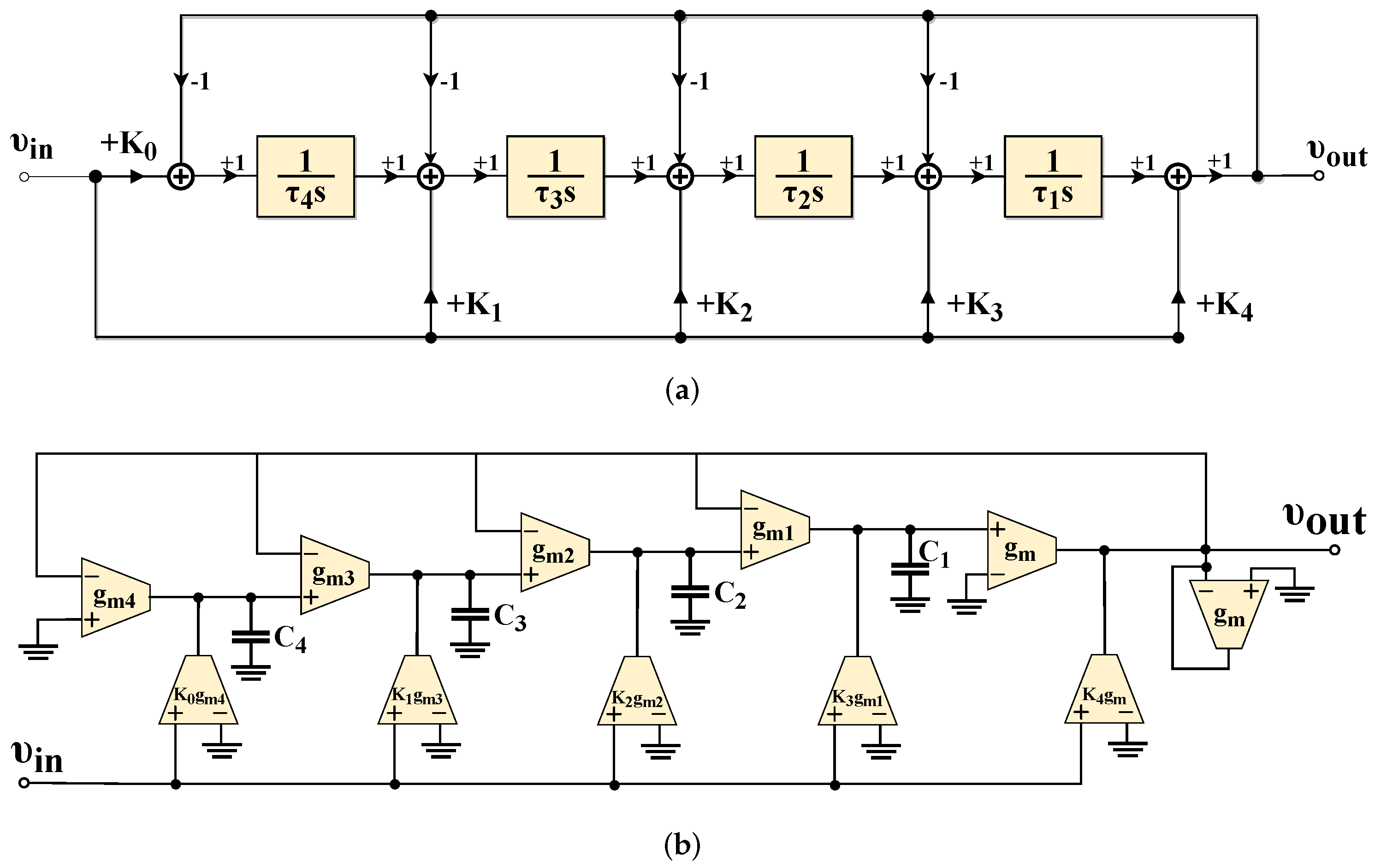
4. Proposed Electronically Tunable Scheme for Realizing all Possible Filter Functions

4.1. Transfer Functions of Filters Derived from 1st-Order Mother Functions

Following the main derivation of the previous section about the employed approximation tool, the transfer functions which approximate the low-pass filters, described by (3) for ω 0 = 1 rad / s , in the range 10 2 , 10 + 2 rad / s for orders {0.3, 0.5, 0.7}, are given by:
H L P , 03 ( s ) = 0.1568 s 4 + 28.89 s 3 + 638.2 s 2 + 2945 s + 3066 s 4 + 88.25 s 3 + 1202 s 2 + 3864 s + 3066 ,
H L P , 05 ( s ) = 0.0438 s 4 + 10.72 s 3 + 262.3 s 2 + 1298 s + 1435 s 4 + 66.8 s 3 + 733.4 s 2 + 2016 s + 1435 ,
H L P , 07 ( s ) = 0.0106 s 4 + 4.098 s 3 + 112.8 s 2 + 600.4 s + 704.2 s 4 + 51.23 s 3 + 459.5 s 2 + 1093 s + 704.2 .
In the case of the 1st-order high-pass mother function, described by (6), the corresponding approximate transfer functions are provided in:
H H P , 03 ( s ) = s 4 + 0.9605 s 3 + 0.2082 s 2 + 0.009421 s + 5.144 · 10 5 s 4 + 1.26 s 3 + 0.3922 s 2 + 0.02878 s + 0.0003261 ,
H H P , 05 ( s ) = s 4 + 0.9049 s 3 + 0.1828 s 2 + 0.00747 s + 3.053 · 10 5 s 4 + 1.405 s 3 + 0.5111 s 2 + 0.04655 s + 0.0006969 ,
H H P , 07 ( s ) = s 4 + 0.8526 s 3 + 0.1601 s 2 + 0.00582 s + 1.505 · 10 5 s 4 + 1.552 s 3 + 0.6525 s 2 + 0.07276 s + 0.00142 .

4.2. Transfer Functions of Filters Derived from 2nd-Order Mother Functions

Considering 2nd-order mother functions with ω 0 = 1 rad / s and Q = 1 , the approximate transfer functions, for orders {0.3,0.5,0.7} are given by (22a)–(22c) in the case of LP filter, by (23a)–(23c) for HP filters, by (24a)–(24c) for BP filters, and by (25a)–(25c) for BS filters, as:
H L P , 03 ( s ) = 0.03255 s 4 + 4.863 s 3 + 48.35 s 2 + 81.03 s + 65.05 s 4 + 25 s 3 + 85.6 s 2 + 100.4 s + 65.06 ,
H L P , 05 ( s ) = 1.59 · 10 5 s 4 + s 3 + 2.528 s 2 + 2.619 s + 1.136 s 4 + 3.026 s 3 + 4.266 s 2 + 3.187 s + 1.136 ,
H L P , 07 ( s ) = 0.002071 s 4 + 0.2282 s 3 + 3.868 s 2 + 7.942 s + 4.775 s 4 + 6.974 s 3 + 12.23 s 2 + 11.29 s + 4.775 .
H H P , 03 ( s ) = s 4 + 1.246 s 3 + 0.7432 s 2 + 0.07475 s + 0.0005004 s 4 + 1.544 s 3 + 1.316 s 2 + 0.3842 s + 0.01537 ,
H H P , 05 ( s ) = s 4 + 2.306 s 3 + 2.226 s 2 + 0.88 s + 1.399 · 10 5 s 4 + 2.806 s 3 + 3.756 s 2 + 2.664 s + 0.8804 ,
H H P , 07 ( s ) = s 4 + 1.663 s 3 + 0.8101 s 2 + 0.04779 s 0.0004336 s 4 + 2.365 s 3 + 2.562 s 2 + 1.461 s + 0.2094 .
H B P , 03 ( s ) = 0.2162 s 4 + 11.61 s 3 + 39.28 s 2 + 11.61 s + 0.2162 s 4 + 22 s 3 + 41.35 s 2 + 22 s + 1 ,
H B P , 05 ( s ) = 0.07688 s 4 + 5.357 s 3 + 20.23 s 2 + 5.357 s + 0.07688 s 4 + 14.73 s 3 + 22.32 s 2 + 14.73 s + 1 ,
H B P , 07 ( s ) = 0.02413 s 4 + 2.638 s 3 + 11.22 s 2 + 2.638 s + 0.02413 s 4 + 10.21 s 3 + 13.26 s 2 + 10.21 s + 1 .
H B S , 03 ( s ) = s 4 + 0.5203 s 3 + 2.023 s 2 + 0.5203 s + 0.9998 s 4 + 0.8173 s 3 + 2.082 s 2 + 0.8173 s + 1 ,
H B S , 05 ( s ) = s 4 + 0.4608 s 3 + 2.015 s 2 + 0.4608 s + 0.9998 s 4 + 0.9578 s 3 + 2.129 s 2 + 0.9578 s + 1 ,
H B S , 07 ( s ) = s 4 + 0.4025 s 3 + 2.008 s 2 + 0.4025 s + 0.9999 s 4 + 1.1 s 3 + 2.191 s 2 + 1.1 s + 1 .

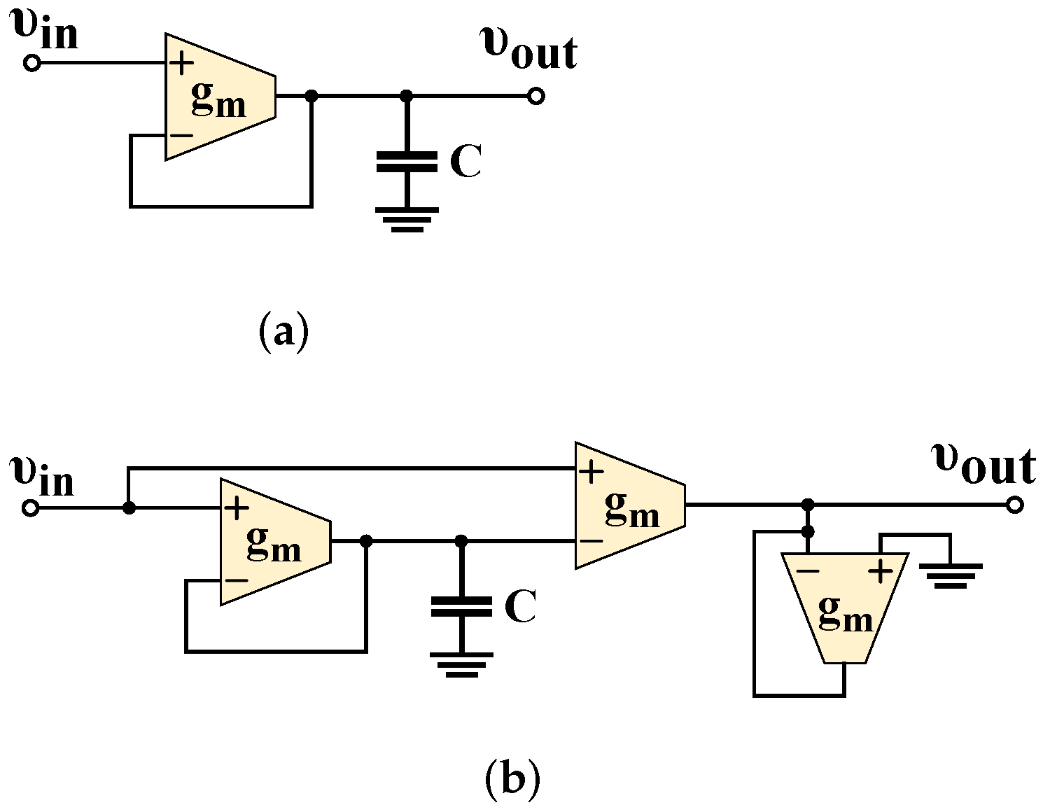
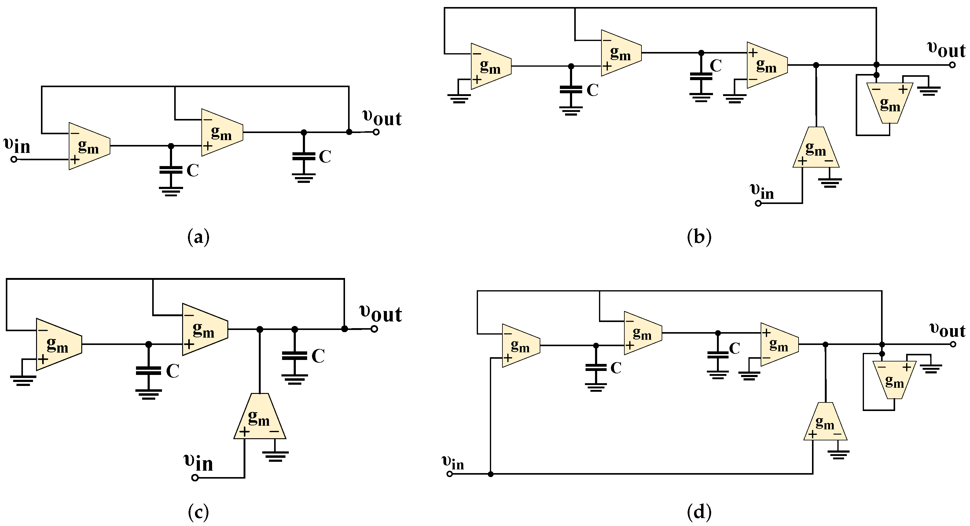
4.3. OTA-C Controllable Structure for Approximating the Behavior of Power-Law Filters

As the transfer functions in Section 4.1 and Section 4.2 have the same form, their implementation can be performed through the employment of conventional integer-order techniques. An efficient realization option is described by the Functional Block Diagram (FBD) in Figure 3a, which represents an IFLF structure. The associated transfer function is given by:
H I F L F ( s ) = K 4 · s 4 + K 3 τ 1 · s 3 + K 2 τ 1 τ 2 · s 2 + K 1 τ 1 τ 2 τ 3 · s + K 0 τ 1 τ 2 τ 3 τ 4 s 4 + 1 τ 1 · s 3 + 1 τ 1 τ 2 · s 2 + 1 τ 1 τ 2 τ 3 · s + 1 τ 1 τ 2 τ 3 τ 4 .
The employment of OTAs as active elements for realizing (26) offers the advantages of higher frequency ranges and simpler tuning than those offered by the corresponding RC implementations where active elements such as op-amps, CFOAs, etc., are utilized. These are originated from the fact that OTAs do not require frequency compensation due to their simple structures and from the employment of the electronically controlled transconductance parameter, respectively. In addition, the OTA-C filter structures have capability of monolithic implementation, reducing the cost of mixed-signal systems. On the other hand, the effect of parasitics, the changes of transconductance with frequency variations, and the reduction of linearity which originated from the small-signal nature of the transconductance are the drawbacks of the employment of these active elements [24]. The OTA-C implementation of (26) is depicted in Figure 3b, where the realized time constants are given by:
τ j = C j g m j j = 1 , , 4 .
The calculation of the values of coefficients K i , ( i = 0 , 1 , , 4 ), and τ j , ( j = 1 , 2 , , 4 ), are calculated equating the coefficients of both numerator and denominator in (20a)–(25c) with those of (26).
In cases where orders 1 < α < 2 are required, this can be implemented by cascading the structure in Figure 3b and one of of stages that implement the corresponding mother filter function. In order to facilitate the reader, the 1st-order OTA-C LP and HP mother filter structures are depicted in Figure 4, while the corresponding 2nd-order OTA-C LP, HP, BP, and BS mother filter implementations are provided in Figure 5 [25].
This can be further generalized, in the sense that an n + α -order power-law filter, where n is an integer and 0 < α < 1 , can be implemented through the cascade connection of n mother filter stages with the filter in Figure 3b, which implements the decimal part of the order.

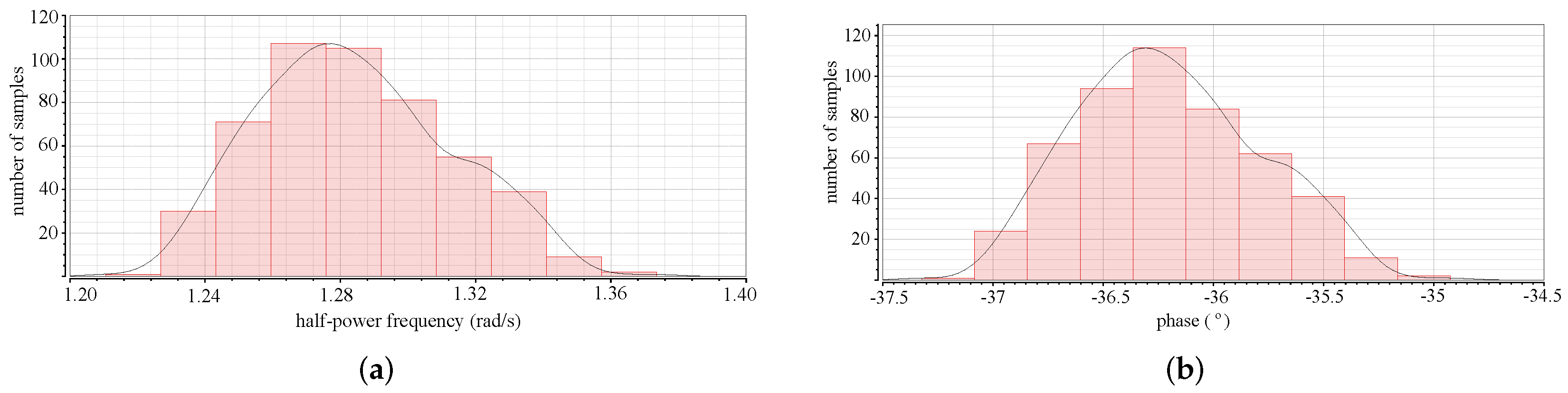
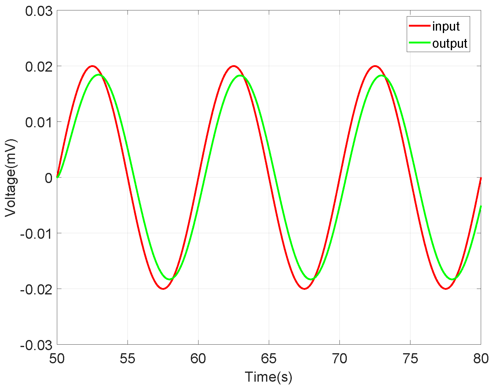
5. Simulation Results

The performance of the proposed implementation of a generalized power-law filter will be evaluated in Cadence IC design suite, using the design kit provided by the Austria Mikro Systeme (AMS) CMOS 0.35 μ m process. The OTA-based structure, employed in simulations, is depicted in Figure 6 [26], while the MOS transistors aspect ratios for V D D = V S S = 0.75 V are summarized in Table 1. The provided electronic tunability is originated from the transconductance of the OTA which is given by the following expression:
g m = 5 I B 9 n V T ,
with n being the slope factor of a MOS transistor in sub-threshold region (1 < n < 2), V T being the thermal voltage (26 mV at 27 C), and I B being the DC bias current, making the time constants in (27), as well as the required scaling factors, electronically adjustable. The layout design of the active core is provided in Figure 7.

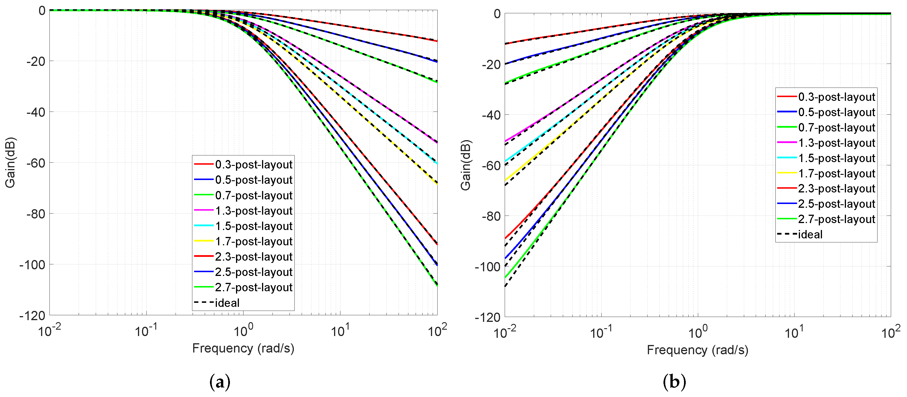
5.1. Results of Filters Derived from 1st-Order Mother Functions

Equating the coefficients of (20a)–(21c) with the ones of (26), the calculated values of the scaling factors K i ( i = 0 , 1 , , 5 ) are summarized in Table 2. Assuming a minimum bias current equal to I B = 50 pA , for avoiding problems related to leakage currents, then using (28) the resulting values of transconductances associated with the integration and summation stages are also given in the same Table. The values of capacitances can be easily calculated using (27), with the values of time constants being available through the expressions of the coefficients in (20a)–(21c).
The obtained post-layout frequency responses of orders {0.3, 0.5, 0.7, 1.3, 1.5, 1.7, 2.3, 2.5, 2.7} are provided in the plots of Figure 8. It must be mentioned at this point that the orders greater than one have been implemented using the building blocks of Figure 4 with ω 0 = 1 rad / s . The critical performance factors, summarized in Table 3, confirm the accurate operation of the proposed scheme. With regards to the time-domain behavior of the presented filters, the output voltage waveform along with the associated input waveform of an LP filter of order equal to 0.5, stimulated by a 20 mV, 0.1 Hz sinusoidal input, are depicted in Figure 9. The measured values of gain and phase difference were 0.923, −15.54°, close to the theoretically predicted values 0.92 and −15.6°.
Considering LP filters of order {0.5, 1.5, 2.5}, the corresponding values of power dissipation were 14.077 nW, 14.308 nW, and 14.541 nW. With regards to the linear performance of these filters, a 1% Total Harmonic Distortion (THD) has been observed at levels 26.28 mV, 27.5 mV, and 29.3 mV, respectively. The Root Mean Square (RMS) values of the input refereed noise, integrated within the pass band, have been measured as 0.326 nV, 0.349 nV, and 0.421 nV for the considered orders. Consequently, the predicted values of the dynamic range (DR) will be 155.1 dB, 154.9 dB, and 153.8 dB, respectively.
The sensitivity performance of the filters has been evaluated using the Monte-Carlo analysis tool, for N = 500 runs. Indicatively, the results for the characteristic half-power frequency and the phase at this frequency, in the case of the low-pass filter of order α = 0.7 , are depicted in Figure 10. In particular, for the half-power frequency the standard deviation is equal to 0.028 rad/s with a mean value equal to 1.284 rad/s, while for the phase at the half-power frequency the standard deviation is equal to 0.41 with a mean value equal to −36.2 .

5.2. Results of Filters Derived from 2nd-Order Mother Functions

Following a similar procedure as in the previous sub-section and considering 2nd-order mother functions with ω 0 = 1 rad / s and Q = 1 , the design parameters of LP, HP, BP, and BS filters are summarized in Table 4 and Table 5. The corresponding post-layout frequency responses alongside the most important performance factors are provided in Figure 11 and Figure 12 and Table 6 and Table 7, respectively. The LP and HP filter responses have been shifted to ω 0 = 100 rad / s , and from the provided plots it is evident the deviation form the ideal responses in the relatively high frequencies, caused by the MOS transistor performance degradation as they are biased in the sub-threshold region. The bandwidth of the BP and BS filters is defined as B W ω h , u ω h , l , with ω h , l and ω h , u being the low and high half-power frequencies, respectively, while the quality (Q) factor is given by the expression: Q = ω p e a k / B W . The input and output voltage waveforms of a LP filter ( α = 0.5) stimulated by a 20 mV, 10 Hz sinusoidal input are provided in Figure 13. According to these plots, the gain is equal to 1.06, while the phase difference is −23.81°. As the corresponding theoretically predicted values are 1.07 and −23.99°, the accurate operation of the filters from the time-domain point of view is also verified.
The values of the power dissipation, in the case of LP filters of order {0.5, 1.5, 2.5}, were 2.985 nW, 3.45 nW, and 3.913 nW, respectively. The levels of the input signal, where 1% THD has been measured were 27.6 mV, 22.6 mV, and 21.2 mV, respectively. The integrated noise RMS values were 12.95 nV, 10.58 nV, and 10.60 nV and, therefore, the predicted values of the DR will be 123.6 dB for orders {0.5, 1.5}, and 123 dB for order 2.5.
The statistical plots in the case of a BP filter of order α = 0.7 are shown in Figure 14, and the derived values of the standard deviation of the bandwidth of the filters are equal to 0.028 rad/s with a mean value being 1.37 rad/s, while for the Q factor the standard deviation is equal to 0.015 with a mean value equal to 0.73.

6. Conclusions

Different approximation tools have been evaluated in this work, for choosing the most efficient for approximating the behavior of power-law filters. It was found that the curve-fitting-based technique based on the fitfrd command of MATLAB is the best option and the derived integer-order rational transfer functions can be implemented using conventional filter design techniques.
In order to achieve electronic adjustability of the realized filter functions, the small-signal transconductance parameter is a suitable choice towards this goal. In this work, OTAs have been selected as active elements, where their transconductance is controlled by a bias current.
The derived OTA-C structure is versatile, in the sense that the standard filter functions can be implemented by the same active core, after changing the values of the bias currents. This is independent of the order, as well as of the type of the mother filter function. The provided post-layout simulation results confirm that the presented structure is both accurate and robust.
Future research steps include the exploitation of alternative electronically controlled active elements, as well as of other design techniques, in order to reduce the complexity of the overall structure, which is the price paid for the offered design flexibility and versatility.

Author Contributions

Conceptualization, C.P., S.K. and A.S.E.; methodology, E.T., S.K. and D.J.; software, E.T.; validation, E.T.; formal analysis, E.T.; investigation, E.T.; writing—original draft preparation, E.T., S.K. and C.P; writing—review and editing, S.K., A.S.E. and D.J.; project administration, C.P. and S.K. All authors have read and agreed to the published version of the manuscript.

Funding

This research received no external funding.

Institutional Review Board Statement

Not applicable.

Informed Consent Statement

Not applicable.

Data Availability Statement

No new data were created or analyzed in this study. Data sharing is not applicable to this article.

Conflicts of Interest

The authors declare no conflict of interest.

Abbreviations

The following abbreviations are used in this manuscript:
AMS  Austria Mikro Systeme
BP  Band-Pass
BS  Band-Stop
BW  Bandwidth
CFOA  Current Feedback Operational Amplifier
CMOS  Complementary Metal Oxide Semiconductor
DR  Dynamic Range
FO  Fractional-Order
FBD  Functional Block Diagram
FLF  Follow the Leader Feedback
HP  High-Pass
IC  Integrated Circuits
IFLF  Inverse Follow the Leader Feedback
LP  Low-Pass
MOS  Metal Oxide Semiconductor
OP-AMP  Operational Amplifier
OΤA  Operational Transconductance Amplifier
OTA-C  Operational Transconductance Amplifier-Capacitor
PL  Power-Law
Q factor  Quality factor
RMS  Root Mean Square
THD  Total Harmonic Distortion

References

  1. Radwan, A.G.; Khanday, F.A.; Said, L.A. Fractional-Order Design: Devices, Circuits, and Systems; Elsevier: Amsterdam, The Netherlands, 2021. [Google Scholar]
  2. Mahata, S.; Saha, S.; Kar, R.; Mandal, D. Optimal integer-order rational approximation of α and α+ β fractional-order generalised analogue filters. IET Signal Process. 2019, 13, 516–527. [Google Scholar] [CrossRef]
  3. Mahata, S.; Kar, R.; Mandal, D. Optimal approximation of fractional-order systems with model validation using CFOA. IET Signal Process. 2019, 13, 787–797. [Google Scholar] [CrossRef]
  4. Mahata, S.; Kar, R.; Mandal, D. Optimal approximation of asymmetric type fractional-order bandpass Butterworth filter using decomposition technique. Int. J. Circuit Theory Appl. 2020, 48, 1554–1560. [Google Scholar] [CrossRef]
  5. Mahata, S.; Herencsar, N.; Kubanek, D. Optimal Approximation of Fractional-Order Butterworth Filter based on Weighted Sum of Classical Butterworth Filters. IEEE Access 2021, 9, 81097–81114. [Google Scholar] [CrossRef]
  6. Colín-Cervantes, J.D.; Sánchez-López, C.; Ochoa-Montiel, R.; Torres-Muñoz, D.; Hernández-Mejía, C.M.; Sánchez-Gaspariano, L.A.; González-Hernández, H.G. Rational Approximations of Arbitrary Order: A Survey. Fractal Fract. 2021, 5, 267. [Google Scholar] [CrossRef]
  7. Kapoulea, S.; Psychalinos, C.; Elwakil, A.S. Power law filters: A new class of fractional-order filters without a fractional-order Laplacian operator. AEU-Int. J. Electron. Commun. 2021, 129, 153537. [Google Scholar] [CrossRef]
  8. Agarwal, P.; Baleanu, D.; Chen, Y.; Momani, S.; Machado, J.A.T. Fractional Calculus. In Proceedings of the Conference ICFDA 2018, Amman, Jordan, 16–18 July 2018; Springer Nature Singapore Pte Ltd.: Singapore, 2018; p. 5. [Google Scholar]
  9. Kapoulea, S.; Yesil, A.; Psychalinos, C.; Minaei, S.; Elwakil, A.S.; Bertsias, P. Fractional-Order and Power-Law Shelving Filters: Analysis and Design Examples. IEEE Access 2021, 9, 145977–145987. [Google Scholar] [CrossRef]
  10. Kapoulea, S.; Psychalinos, C.; Elwakil, A.S.; Tavazoei, M.S. Power-Law Compensator Design for Plants with Uncertainties: Experimental Verification. Electronics 2021, 10, 1305. [Google Scholar] [CrossRef]
  11. Ozdemir, A.A.; Gumussoy, S. Transfer function estimation in system identification toolbox via vector fitting. IFAC-PapersOnLine 2017, 50, 6232–6237. [Google Scholar] [CrossRef]
  12. Bingi, K.; Ibrahim, R.; Karsiti, M.N.; Hassan, S.M.; Harindran, V.R. Fractional-Order Systems and PID Controllers; Springer Nature Switzerland AG: Cham, Switzerland, 2020. [Google Scholar]
  13. Mahata, S.; Herencsar, N.; Kubanek, D. On the Design of Power Law Filters and Their Inverse Counterparts. Fractal Fract. 2021, 5, 197. [Google Scholar] [CrossRef]
  14. Baxevanaki, K.; Kapoulea, S.; Psychalinos, C.; Elwakil, A.S. Electronically tunable fractional-order highpass filter for phantom electroencephalographic system model implementation. AEU-Int. J. Electron. Commun. 2019, 110, 152850. [Google Scholar] [CrossRef]
  15. Said, L.A.; Ismail, S.M.; Radwan, A.G.; Madian, A.H.; El-Yazeed, M.F.A.; Soliman, A.M. On the optimization of fractional order low-pass filters. Circuits, Syst. Signal Process. 2016, 35, 2017–2039. [Google Scholar] [CrossRef]
  16. Matsuda, K.; Fujii, H. H optimized wave-absorbing control—Analytical and experimental results. J. Guid. Control. Dyn. 1993, 16, 1146–1153. [Google Scholar] [CrossRef]
  17. Oustaloup, A.; Levron, F.; Mathieu, B.; Nanot, F.M. Frequency-band complex noninteger differentiator: Characterization and synthesis. IEEE Trans. Circuits Syst. I Fundam. Theory Appl. 2000, 47, 25–39. [Google Scholar] [CrossRef]
  18. Krishna, B.T. Studies on fractional order differentiators and integrators: A survey. Signal Process. 2011, 91, 386–426. [Google Scholar] [CrossRef]
  19. El-Khazali, R. On the biquadratic approximation of fractional-order Laplacian operators. Analog Integr. Circuits Signal Process. 2015, 82, 503–517. [Google Scholar] [CrossRef]
  20. Koseoglu, M.; Deniz, F.N.; Alagoz, B.B.; Alisoy, H. An effective analog circuit design of approximate fractional-order derivative models of M-SBL fitting method. Eng. Sci. Technol. Int. J. 2021, 33, 101069. [Google Scholar] [CrossRef]
  21. Lorentzen, L. Padé approximation and continued fractions. Appl. Numer. Math. 2010, 60, 1364–1370. [Google Scholar] [CrossRef]
  22. Barbé, K. Measurement of Cole–Davidson diffusion through Padé approximations for (bio) impedance spectroscopy. IEEE Trans. Instrum. Meas. 2019, 69, 301–310. [Google Scholar] [CrossRef]
  23. Brezinski, C. History of Continued Fractions and Padé Approximants; Springer: Berlin/Heidelberg, Germany, 2012; Volume 12. [Google Scholar]
  24. Sánchez-Gaspariano, L.A.; Muñiz-Montero, C.; Muñoz-Pacheco, J.M.; Sánchez-López, C.; Gómez-Pavón, L.d.C.; Luis-Ramos, A.; Bautista-Castillo, A.I. CMOS analog filter design for very high frequency applications. Electronics 2020, 9, 362. [Google Scholar] [CrossRef] [Green Version]
  25. Mohan, P.A. VLSI Analog Filters: Active RC, OTA-C, and SC; Springer Science & Business Media: New York, NY, USA, 2012. [Google Scholar]
  26. Corbishley, P.; Rodriguez-Villegas, E. A nanopower bandpass filter for detection of an acoustic signal in a wearable breathing detector. IEEE Trans. Biomed. Circuits Syst. 2007, 1, 163–171. [Google Scholar] [CrossRef] [PubMed]
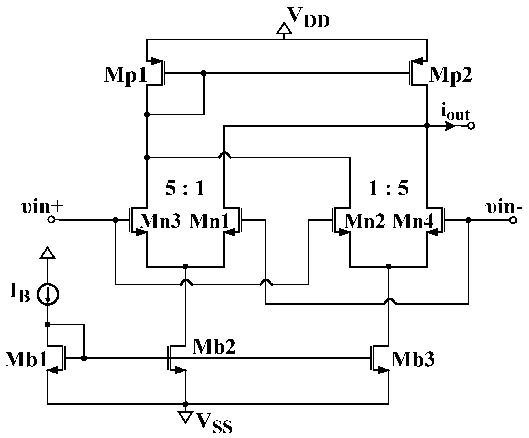
Figure 1. Frequency responses of the (a) gain and (b) phase of an approximate LP filter with α = 0.3 , using a 4th-order approximation.
Fractalfract 06 00111 g001
Figure 2. Error plots of the (a) gain and (b) phase of an approximate LP filter with α = 0.3 , using a 4th-order approximation.
Fractalfract 06 00111 g002
Figure 3. (a) Functional block diagram of an IFLF structure and (b) OTA-C structure for implementing the transfer functions in (20a)–(25c).
Fractalfract 06 00111 g003
Figure 4. OTA-C realization of a 1st-order (a) LP, and (b) HP filter.
Fractalfract 06 00111 g004
Figure 5. OTA-C realization of a 2nd-order (a) LP, (b) HP, (c) BP and (d) BS filter.
Fractalfract 06 00111 g005
Figure 6. Operational transconductance amplifier structure used in simulations.
Fractalfract 06 00111 g006
Figure 7. Layout design of the active core in Figure 3b.
Fractalfract 06 00111 g007
Figure 8. Post-layout simulation responses of (a) LP and (b) HP power-law filters, derived from 1st-order mother functions (the ideal ones are provided by dashed lines).
Fractalfract 06 00111 g008
Figure 9. Input and output waveforms of a LP filter ( α = 0.5), derived from a 1st-order mother function, stimulated by a 0.1 Hz, 20 mV signal.
Fractalfract 06 00111 g009
Figure 10. Monte-Carlo analysis results of the (a) half-power frequency and (b) phase at half-power frequency in the case of a LP filter of order α = 0.7 , derived from 1st-order mother function.
Fractalfract 06 00111 g010
Figure 11. Post-layout simulation responses of (a) LP and (b) HP power-law filters derived from 2nd-order mother functions. (with the ideal ones are provided by dashed lines).
Fractalfract 06 00111 g011
Figure 12. Post-layout simulation responses of (a) BP and (b) BS power-law filters derived from 2nd-order mother functions (the ideal ones are provided by dashed lines).
Fractalfract 06 00111 g012
Figure 13. Input and output waveforms of a LP filter ( α = 0.5), derived from a 2nd-order mother function, stimulated by a 10 Hz, 20 mV signal.
Fractalfract 06 00111 g013
Figure 14. Monte-Carlo analysis results of the (a) bandwidth, and (b) Q factor in the case of a BP filter of order α = 0.7, derived from 2nd-order mother function.
Fractalfract 06 00111 g014
Table 1. MOS transistors aspect ratios of the OTA structure in Figure 6.
TransistorsAspect Ratio
Mb1–Mb34.4 μ m/5 μ m
Mp1–Mp20.5 μ m/1.5 μ m
Mn1–Mn21.1 μ m/1.5 μ m
Mn3–Mn45.5 μ m/1.5 μ m
Table 2. Parameters of the filter structure in Figure 3, for implementing various orders derived from 1st-order mother functions.
ParameterLP FilterHP Filter
0.30.50.70.30.50.7
K 0 1110.15680.04380.0106
K 1 0.76210.64420.54920.32730.16050.08
K 2 0.53080.35770.24540.53080.35770.2454
K 3 0.32730.16050.080.76210.64420.5492
K 4 0.15680.04380.0106111
g m 0 (nS)6.6523.8298.461.041.041.04
g m 1 (nS)3.196.513.041.371.621.9
g m 2 (nS)1.972.924.251.972.924.25
g m 3 (nS)1.371.621.93.196.513.04
g m 4 (nS)1.041.041.046.6523.8298.46
Table 3. Frequency characteristics of the filters responses in Figure 8, along with the theoretical values given between parentheses.
OrderLP FilterHP FilterLP FilterHP Filter
ω h (rad/s)phase@ ω h (°)
0.32.99 (3.01)0.30 (0.33)−21.41 (−21.49)21.46 (21.49)
0.51.73 (1.73)0.54 (0.58)−29.84 (−30)29.66 (30)
0.71.3 (1.3)0.73 (0.77)−36.2 (−36.71)36.1 (36.71)
1.30.84 (0.84)1.18 (1.19)−51.88 (−52.01)51.36 (52.01)
1.50.77 (0.77)1.29 (1.3)−56.06 (−56.2)55.5 (56.2)
1.70.71 (0.71)1.4 (1.41)−59.96 (−60.11)59.32 (60.11)
2.30.59 (0.59)1.68 (1.69)−70.42 (−70.5)69.78 (70.5)
2.50.57 (0.57)1.76 (1.77)−73.6 (−73.7)72.87 (73.7)
2.70.54 (0.54)1.84 (1.85)−76.6 (−76.7)75.82 (76.7)
Table 4. Values of scaling factors and transconductances for realizing LP and HP power-law filters derived from 2nd-order mother functions.
ParameterLP FilterHP Filter
0.30.50.70.30.50.7
K 0 1110.03261.59 × 10—5−0.0021
K 1 0.80670.82190.70330.19450.33030.0327
K 2 0.56480.59270.31620.56480.59270.3162
K 3 0.19450.33030.03270.80670.82190.7033
K 4 0.03261.59 × 10—5−0.0021111
g m 0 (nS)32.0565638503.881.041.041.04
g m 1 (nS)5.363.1631.881.291.271.48
g m 2 (nS)1.851.763.31.851.763.3
g m 3 (nS)1.291.271.485.363.1631.88
g m 4 (nS)1.041.041.0432.0565638503.88
Table 5. Values of scaling factors and transconductances for realizing BP and BS power-law filters derived from 2nd-order mother functions.
ParameterBP FilterBS Filter
0.30.50.70.30.50.7
K 0 0.21620.07690.02410.99980.99980.9999
K 1 0.52750.36360.25840.63660.48110.3658
K 2 0.950.90630.84620.97160.94660.9166
K 3 0.52750.36360.25840.63660.48110.3658
K 4 0.21620.07690.02410.99980.99980.9999
g m 0 (nS)4.8313.5743.241.041.041.04
g m 1 (nS)1.982.874.041.642.172.85
g m 2 (nS)1.11.151.231.851.11.14
g m 3 (nS)1.982.874.041.642.172.85
g m 4 (nS)4.8313.5743.241.041.041.04
Table 6. Frequency characteristics of the LP and HP filters responses in Figure 11, along with the theoretical values given between parentheses.
OrderLP FilterHP FilterLP FilterHP Filter
ω h (rad/s)phase@ ω h ( )
0.3185 (189)52 (53)−42.86 (−43.07)42.12 (43.07)
0.5153 (152)65 (66)−65.9 (−65.32)65.39 (65.32)
0.7137 (138)73 (74)−86.39 (−86.11)81.1 (86.11)
1.3121 (121)82 (82)−144.5 (−144.4)142.3 (144.4)
1.5119 (118)83 (83)−163.5 (−163)162.3 (163)
1.7116 (118)86 (85)−182.3 (−183.5)175.8 (183.5)
2.3112 (115)88 (88)−237.3 (−241.7)233.9 (241.7)
2.5111 (111)89 (89)−255.7 (−255.5)253.4 (255.5)
2.7110 (107)90 (90)−272.8 (−267.6)266.22 (267.6)
Table 7. Frequency characteristics of the BP and BS filters responses in Figure 12, along with the theoretical values given between parentheses.
OrderBP FilterBS FilterBP FilterBS FilterBP FilterBS Filter
ω peak (rad/s)Bandwidth (rad/s)Q Factor (rad/s)
0.30.99 (1)0.97 (1)3.03 (3.03)0.34 (0.33)0.33 (0.33)2.94 (3.01)
0.50.99 (1)0.97 (1)1.82 (1.74)0.63 (0.58)0.55 (0.57)1.59 (1.73)
0.70.99 (1)0.97 (1)1.37 (1.31)0.81 (0.77)0.73 (0.76)1.23 (1.3)
1.31 (1)1 (1)0.89 (0.84)1.3 (1.19)1.12 (1.19)0.77 (0.84)
1.51 (1)0.99 (1)0.81 (0.77)1.42 (1.31)1.23 (1.3)0.7 (0.76)
1.71 (1)0.99 (1)0.74 (0.71)1.52 (1.41)1.35 (1.41)0.66 (0.71)
2.31 (1)1 (1)0.62 (0.59)1.88 (1.69)1.61 (1.69)0.53 (0.59)
2.51 (1)1 (1)0.59 (0.56)1.98 (1.77)1.69 (1.78)0.51 (0.56)
2.71 (1)1 (1)0.56 (0.54)2.06 (1.85)1.79 (1.85)0.49 (0.54)
Publisher’s Note: MDPI stays neutral with regard to jurisdictional claims in published maps and institutional affiliations.

