Article

Choosing the Best Members of the Optimal Eighth-Order Petković’s Family by Its Fractal Behavior

School of Mathematical Sciences, Bohai University, Jinzhou 121000, China
*
Author to whom correspondence should be addressed.
Fractal Fract. 2022, 6(12), 749; https://doi.org/10.3390/fractalfract6120749
Submission received: 8 November 2022 / Revised: 9 December 2022 / Accepted: 15 December 2022 / Published: 19 December 2022

Abstract

:
In this paper, by applying Petković’s iterative method to the Möbius conjugate mapping of a quadratic polynomial function, we attain an optimal eighth-order rational operator with a single parameter r and research the stability of this method by using complex dynamics tools on the basis of fractal theory. Through analyzing the stability of the fixed point and drawing the parameter space related to the critical point, the parameter family which can make the behavior of the corresponding iterative method stable or unstable is obtained. Lastly, the consequence is verified by showing their corresponding dynamical planes.

1. Introduction

In 1975, the celebrated scientist Mandelbrot published his monograph Fractals: Form, Chance and Dimension, which marked the birth of fractal geometry [1]. Mandelbrot called the shape of a part similar to the whole in some way fractal. Fractal theory is an extraordinarily popular and active new theory, as well as a new discipline. Its mathematical basis is fractal geometry, which derives fractal information [2,3], fractal design [4,5], fractal art [6] and other applications [7,8] from fractal geometry. The most fundamental characteristic of fractal theory is to describe and study objective things with the perspective of fractional dimension and mathematical methods, that is, to describe and study objective things with the mathematical tools of fractal dimension, which is closer to the description of the real attributes and states of complex systems, as well as more in line with the diversity and complexity of objective things.
Fractal theory is not only the frontier and essential branch of nonlinear science but also a new cross-sectional discipline. It is a fresh mathematical discipline that studies the characteristics of a class of phenomena. Compared with its geometric form, it is more significantly related to differential equations and dynamic system theory [9,10].
Linear fractal is also called self-similar fractal [11]. The self-similarity principle and iterative generation principle are crucial principles of fractal theory. They characterize that a fractal has invariance under the usual geometric transformation, that is, metric independence. Self-similarity starts from the symmetry of different scales, which means recursion.
According to the degree of self-similarity, a fractal can be divided into regular fractal and irregular fractal. Regular fractal refers to the fractal with strict self-similarity, that is, it can be described by a simple mathematical model, such as Cantor set [12], Koch curve [13], Julia set [14], etc. Anomalous fractals are statistically self-similar fractals, such as meandering coastlines, floating clouds, etc. The Julia set was obtained by French mathematicians Gaston Julia and Pierre Fatou after developing the basic theory of complex function iteration.
In fractal theory, the most basic is the Mandelbrot set [15], and it indicates the set of points which are on the complex plane. It is determined by a quadratic multiform f c ( z ) = z 2 + c in the complex, where c C . For every c, f c ( z ) is iterated from z = 0 to generate the following sequence:
{ 0 , f c ( 0 ) , f c ( f c ( 0 ) ) , f c ( f c ( f c ( 0 ) ) ) , } .
The Mandelbrot set is a set that does not extend the above sequence to all c points of infinity. The Julia set [16] is also generated by the iteration of a complex function. Different from the Mandelbrot set, c is a fixed and constant and can be taken arbitrarily. The sequence generated at this time is:
{ z , z 2 + c , ( z 2 + c ) 2 + c , } .
If this sequence diverges, the corresponding z set belongs to the Julia set. Next, we review the basic theory of the Julia set.
Suppose f : C C is a polynomial f ( z ) = a 0 + a 1 z + + a n z n of order n 2 in the complex field. Let
f 0 ( z ) = z , f 1 ( z ) = f ( z ) , f 2 ( z ) = f ( f ( z ) ) , , f n + 1 ( z ) = f ( f n ( z ) ) , .
(1)
If there exists w C such that f ( w ) = w , then w is called a fixed point of f;
(2)
If there are integers p greater than 1 and w C such that f p ( w ) = w , then w is called the periodic point of f. The smallest p such that f p ( w ) = w is called the period of w, and w , f ( w ) , , f p ( w ) is the period p orbit;
(3)
Let w be a periodic point with period p, and ( f p ) ( w ) = λ ;
  • If λ = 0 , then w is a superattracting point;
  • If 0 | λ | < 1 , then w is an attractive point;
  • If | λ | = 1 , then w is a neutral point;
  • If | λ | > 1 , then w is a repulsive point.
The closure of a repulsive periodic point of f is called a Julia set of f. The remainder of the Julia set is called the Fatou set [17].
Based on the above theoretical support, in recent years, a variety of researchers have been committed to using fractals to research the stability of iterative methods [18,19,20]. In this paper, we analyze the dynamic behavior of the optimal eighth-order iterative method proposed by Petković in reference [21]. Its error equation is e k + 1 = c 2 2 ( c 3 + c 2 2 ( 1 + 2 r ) ) ( c 2 c 3 + c 4 + c 2 3 ( 1 + 2 r ) ) e k 8 + O ( e k 9 ) , and its specific iterative scheme is as follows:
y k = x k f ( x k ) f ( x k ) , z k = y k f ( y k ) f ( x k ) f ( x k ) + r f ( y k ) f ( x k ) + ( r 2 ) f ( y k ) , x k + 1 = z k f ( z k ) H ( z k ) ,
where H ( z k ) = 2 ( f [ x k , z k ] f [ x k , y k ] ) + f [ y k , z k ] + y k z k y k x k ( f [ x k , y k ] f ( x k ) ) , r C and f [ · , · ] is a forward divided difference of order one.
The remainder of the paper is arranged as follows. In Section 2, several fundamental conclusions on Riemann sphere C ˜ are introduced, which are the basis of the subsequent dynamic analysis. The details of the complex dynamic analysis of (1) are described in Section 3. Based on Möbius conjugate theory, we firstly obtain the rational operator related to (1). After that, we utilize the principle that the fixed point and the critical point appear in pairs on the Riemann sphere C ˜ to analyze their stability and draw the fixed point stability surface and the parameter space related to the critical point, so as to attain stable parameters and unstable parameter ranges. In addition, the dynamic behavior of the corresponding iterative method (1) is analyzed by the dynamical planes of the given parameters, and the stable parameter family is finally determined. At last, we summarize the work we conducted.

2. Some Concepts and Properties Related to Riemann Sphere C ˜

In this section, we consider expressing (1) as a nonlinear recurrence form
x k + 1 = R f ( x k ) , k = 0 , 1 , 2 , ,
where R f is an iteration function, as well as a fixed point operator [22]. If the iteration exponent n is used to represent the time index, then the nonlinear recurrence relation (2) will represent the relevant discrete dynamical system. Therefore, the process of solving the solution of the nonlinear equation f ( x ) = 0 can be expressed as an image sequence of the initial guess x 0 under the action of R f :
{ x 0 , R f ( x 0 ) , R f 2 ( x 0 ) , , R f n ( x 0 ) , } .
It can be viewed as a discrete dynamical system. Generally, the iteration function R f is a meromorphic function. According to the Lemma 2.1 of reference [23], the meromorphic functions on Riemann sphere C ˜ can be expressed as rational functions. This solves the difficult problem of directly studying the dynamics of meromorphic functions. Here, the related properties of the topological conjugate are also necessary to be mentioned.
Definition 1. 
Let F be a function of the set X and G be a function defined on the set Y. If there exists an isomorphism h satisfying F h = h G , then F is conjugate to G through h.
Theorem 1. 
Let F , G C 1 and there exist conjugate h such that F h = h G . Consider α to be a fixed point of G , then the following results hold:
( a ) Under topological conjugate h, the fixed point property remains unchanged, namely,
α = G ( α ) h ( α ) = F ( h ( α ) ) .
( b ) Let m ( G , α ) denote the Poincaré characteristic multiplier [24] of α by G . It remains unchanged under the diffeomorphic conjugate h, that is,
m ( h G h 1 , h ( α ) ) = F ( h ( α ) ) = G ( α ) = m ( G , α ) .
Proof. 
( a ) Derives from α = G ( α ) ,
h G ( α ) = h ( α ) = F ( h ( α ) ) = F ( h ( α ) ) ,
and vice versa.
( b ) For z Y , there is
h G ( z ) = F h ( z ) ,
namely,
h ( G ( z ) ) = F ( h ( z ) ) .
Find the first derivative of z and obtain
[ h ( G ( z ) ) ] = h ( G ( z ) ) · G ( z ) .
Let z = α ,
[ h ( G ( α ) ) ] = h ( G ( α ) ) · G ( α ) = h ( α ) G ( α ) = F ( h ( α ) ) · h ( α )
holds. Since h ( α ) 0 , F ( h ( α ) ) = G ( α ) . □
Lemma 1. 
Let ω : U C ¯ U be meromorphic and η U be a fixed point with | ω ( η ) | < 1 . Then ω has a unique fixed point η such that the sequence { z n + 1 = ω ( z n ) } 0 converges to η for any given z 0 U .
Proof. 
( i ) For η U C , from the analyticity at η ,
z n + 1 η = ω ( z n ) ω ( η ) = ( z n η ) ( ω ( η ) + τ ) ,
when z n η , τ 0 .
N > 0 , ∃ constant β satisfying 0 < β = | ω ( η ) | + | τ | < 1 , s . t . n N , k N { 0 } , we have: | z N + k + 1 η | = | ω ( z N + k ) ω ( η ) | = | z N + k η | | ω ( η ) + τ | | z N + k η | ( | ω ( η ) | + | τ | ) = β | z N + k η | β 2 | z N + k 1 η | β N + k + 1 | z 0 η | .
So, lim k | z N + k + 1 η | = 0 . That is, lim n z n = η .
Suppose ζ η is also a fixed point satisfying lim n z n = ζ . Since the convergent sequence only has a unique limit, ζ = η , contradicting the hypothesis, uniqueness is proven.
( i i ) For ω ( ) = , by definition from Section 3.1 of reference [25], ω is said to be analytic at when H ω H 1 is analytic at 0 with H ( z ) = 1 z . Express ω ( z ) = a 0 + a 1 z + + a n z n b 0 + b 1 z + + b m z m as a rational function with a n b m 0 , n > m for n , m N { 0 } . If we define a function
K ( z ) = H ω H 1 ( z ) = 1 ω ( 1 z )
and find
ω ( ) = K ( 0 ) = b m / a n , if n = m + 1 0 , if n > m + 1
by computation directly. Therefore, if restriction | ω ( ) | = | b m a n | < 1 is made, then becomes an attractive fixed point of ω . □

3. Complex Dynamics Analysis

Based on the conclusion of Section 2, we discuss the dynamic analysis of (1), analyze the stability of this iterative method and find the stable parameter family.

3.1. Fixed Points and Their Stability

By applying any quadratic polynomial f ( z ) = ( z a ) ( z b ) , a b to (1), it can be obtained that
S ( z ; r , a , b ) = C ( z ; r , a , b ) D ( z ; r , a , b ) ,
where C and D are related to a , b , r , z , and then through the Möbius transformation t ( z ) = z a z b and its inverse map t 1 ( z ) = z b a z 1 , it can be obtained that the fixed point operator
M ( z ; r ) = ( t S t 1 ) ( z ) = z 8 ( ( 1 + z ) 2 + r ( 2 + z ) ) 2 ( 1 + ( 2 + r ) z + ( 1 + 2 r ) z 2 ) 2
where M ( z ; r ) is only related to r and z.
Lemma 2. 
Relation M ( z ; r ) · M ( 1 z ; r ) = 1 holds, r C , z C ˜ .
Proof. 
This Lemma is proved by Theorem 1 ( a ) . Under the conjugate mapping h ( z ) = 1 z , M ( z ; r ) is isomorphic to itself, that is to say, z C ˜ , r C ,
M ( z ; r ) h ( z ) = M ( 1 z ; r ) = h ( z ) M ( z ; r ) = 1 M ( z ; r )
holds. Therefore, M ( 1 z ; r ) = 1 M ( z ; r ) , namely, M ( 1 z ; r ) · M ( z ; r ) = 1 . □
Lemma 2 plays an important role in discussing fixed points and critical points. Next, we analyze the fixed points of M ( z ; r ) . Firstly, according to the definition of fixed point and (5), we have
M ( z ; r ) z = z ( z 1 ) · N ( z ; r ) Q ( z ; r ) 2 ,
where N ( z ; r ) = 1 + ( 5 + 2 r ) z + ( 11 + 10 r + r 2 ) z 2 + 5 ( 3 + 4 r + r 2 ) z 3 + ( 4 + 3 r ) 2 z 4 + ( 4 + 3 r ) 2 z 5 + ( 4 + 3 r ) 2 z 6 + 5 ( 3 + 4 r + r 2 ) z 7 +   ( 11 + 10 r + r 2 ) z 8 + ( 5 + 2 r ) z 9 + z 10 and Q ( z ; r ) = 1 + ( 2 + r ) z + ( 1 + 2 r ) z 2 .
Obviously, no matter what value the parameter r takes, z = 0 , z = are fixed points of M ( z ; r ) . z = 0 , z = correspond to the two roots a , b of f ( z ) = ( z a ) ( z b ) , respectively. In fact, the orbits of such fixed points are close to themselves, and it is of little significance to study such fixed points. We are always interested in fixed points other than z = 0 and z = , that is, strange fixed points. By analyzing the strange fixed point and its stability, we can find in the approximate region of the parameters that the sequence generated by the initial point does not converge to the strange fixed point during the iteration process.
Lemma 3. 
Relation N ( 1 z ; r ) = N ( z ; r ) z 10 holds, r C , and z C ˜ .
Corollary 1. 
If z is a fixed point of M ( z ; r ) , then so is 1 z .
Proof. 
Let X = Y = C ˜ , F = G = M and conjugate mapping h ( z ) = 1 z in Theorem 1 ( a ) , the conclusion obviously holds. □
It can be seen from (6) that the strange fixed points of M ( z ; r ) are ten roots of polynomial N ( z ; r ) = 0 and z = 1 , and there are at most eleven strange fixed points. These strange fixed points are denoted by E x i ( i = 1 , 2 , , 11 ) , where E x 1 = 1 denotes z = 1 and E x i ( i = 2 , 3 , , 11 ) denote the ten roots of N ( z ; r ) = 0 in turn. By Corollary 1, our study of the ten roots of the polynomial N ( z ; r ) = 0 can be reduced to half for stability studies. Then, we analyze the existence of common factors in N ( z ; r ) and Q ( z ; r ) in (6). The following theorem describes this conclusion well.
Theorem 2. 
For N ( z ; r ) and Q ( z ; r ) , we can obtain the following conclusions:
( a ) When r = 4 3 , N ( z ; r ) and Q ( z ; r ) have a common factor ( z 1 ) ;
( b ) When r = 0 , N ( z ; r ) and Q ( z ; r ) have a common factor ( 1 + z ) 2 ;
( c ) When r = 28 13 , N ( z ; r ) has a factor ( z 1 ) ;
( d ) When r ( 4 + 3 r ) ( 28 + 13 r ) 0 , the strange fixed points are z = 1 and the roots of N ( z ; r ) = 0 , r C .
Proof. 
By supposing that N ( z ; r ) = 0 and Q ( z ; r ) = 0 for some values of z and eliminating r in N ( z ; r ) = 0 and Q ( z ; r ) = 0 , we obtain ( z 1 ) ( 1 + z ) 6 = 0 . Therefore, ( z 1 ) , ( 1 + z ) and ( 1 + z ) 2 may be common factors.
Considering N ( 1 ; r ) = 39 r 2 + 136 r + 112 = ( 4 + 3 r ) ( 28 + 13 r ) = 0 and Q ( 1 ; r ) = 4 + 3 r = 0 , then when r = 4 3 , ( z 1 ) is a common factor of N ( z ; 4 3 ) and Q ( z ; 4 3 ) . And if r = 28 13 , N ( z ; 28 13 ) has a factor ( z 1 ) , while Q ( z ; 28 13 ) = 1 13 ( 13 2 z 43 z 2 ) . When r = 0 , Q ( z ; 0 ) = ( 1 + z ) 2 , N ( z ; 0 ) = ( 1 + z ) 4 ( 1 + z + z 2 + z 3 + z 4 + z 5 + z 6 ) . That is, when r = 0 , ( 1 + z ) 2 is a common factor of N ( z ; 0 ) and Q ( z ; 0 ) .
( a ) If r = 4 3 , M ( z ; 4 3 ) z = z ( z 1 ) ( 9 + 39 z + 64 z 2 + 64 z 3 + 64 z 4 + 64 z 5 + 64 z 6 + 39 z 7 + 9 z 8 ) ( 3 + 5 z ) 2 . Additionally, the strange fixed points are ( b ) If r = 0 , M ( z ; 0 ) z = z ( z 7 1 ) . At the same time, the strange fixed points are z = 1 , 900969 ± 0.433884 i , 0.62349 ± 0.781831 i , 0.222521 ± 0.974928 i .
( c ) If r = 28 13 , M ( z ; 28 13 ) z =
z ( z 1 ) 3 ( 169 + 455 z 256 z 2 1792 z 3 2304 z 4 1792 z 5 256 z 6 + 455 z 7 + 169 z 8 ) ( 13 + 2 z + 43 z 2 ) 2 . Then, the strange fixed points are z = 1 ( t r i p l e ) , 0.464249 , 2.15402 , 1.83183 ± 0.299321 i , 0.531707 ± 0.0868811 i , 0.291754 ± 0.956493 i .
( d ) The result is obvious. □
Before analyzing the stability of fixed points, it is tremendously necessary to solve the first derivative of M ( z ; r ) , that is,
M ( z ; r ) = 4 z 7 ( 1 + z ) 2 · P ( z ; r ) Q ( z ; r ) 3 ,
where P ( z ; r ) = 2 ( 1 + z ) 4 + 3 r 3 z ( 2 + z ) + 4 r ( 1 + z ) 2 ( 2 + z + z 2 ) + r 2 ( 8 + 11 z + 16 z 2 + 7 z 3 ) . Like the above analysis of fixed points, we are only interested in the behavior of the strange fixed points. The following lemma can be obtained directly by calculation:
Lemma 4. 
Relation P ( 1 z ; r ) = P ( z ; r ) z 4 holds, r C and z C ˜ .
Checking whether P ( z ; r ) and Q ( z ; r ) have common factors, the following theorem describes this property well.
Theorem 3. 
For P ( z ; r ) and Q ( z ; r ) , we can obtain the following conclusions:
( a ) If r = 4 3 , P ( z ; r ) and Q ( z ; r ) have a common factor ( z 1 ) ;
( b ) If r = 0 , ( 1 + z ) 2 is a common factor of P ( z ; r ) and Q ( z ; r ) ;
( c ) If r = 4 , P ( z ; r ) and Q ( z ; r ) all have a factor ( z 1 ) ;
( d ) If r = 2 , P ( z ; r ) has a factor ( z 1 ) 2 ;
( e ) If r = 2 , P ( z ; r ) has a factor ( 1 + z ) 2 ;
( f ) If r = 2 9 or r = 4 15 , P ( z ; r ) has a factor ( 1 + 3 z ) ;
( g ) If r ( 4 + 3 r ) ( r 4 ) ( r + 2 ) ( r 2 ) ( 2 + 9 r ) ( 4 + 15 r ) 0 , according to Theorem 5, the stability of z can be shown graphically by changing the parameter r.
Proof. 
For some value of z, suppose that P ( z ; r ) = 0 and Q ( z ; r ) = 0 . Then, we obtain ( z 1 ) 2 ( 1 + z ) 5 ( 1 + 3 z ) = 0 by eliminating r from P ( z ; r ) = 0 and Q ( z ; r ) = 0 . Additionally, ( z 1 ) , ( z 1 ) 2 , ( 1 + z ) , ( 1 + z ) 2 , ( 1 + 3 z ) are options for common factors. Checking P ( 1 ; r ) = ( 2 + r ) ( 4 + 3 r ) 2 = 0 and Q ( 1 ; r ) = 4 + 3 r = 0 , we obtain r = 4 3 ; ( z 1 ) is a common factor of P ( z ; 4 3 ) and Q ( z ; 4 3 ) . Additionally, if r = 2 , P ( z ; 2 ) has a factor ( z 1 ) while Q ( z ; 2 ) = 1 3 z 2 . By the same treatment, ( b ) ( f ) can be obtained. ( g ) Using Theorem 5, it is easy to express the stability of z by images. □
Corollary 2. 
Relation M ( z ; r ) = M ( 1 z ; r ) holds, r C and z C ˜ is any fixed point of M ( z ; r ) .
Proof. 
Let X = Y = C ˜ , F = G = M , and conjugate mapping h ( z ) = 1 z in Theorem 1 ( b ) , the conclusion obviously holds. □
We now begin to discuss the stability of strange fixed points in two parts. One part is about the stability of E x 1 = 1 , and the other part is about the stability of E x i , i = 2 , 3 , , 11 .
Theorem 4. 
Let r 4 3 , the following results hold:
( a ) | 2 + r 4 + 3 r | > 1 , E x 1 = 1 is a repulsive point;
( b ) | 2 + r 4 + 3 r | = 1 , E x 1 = 1 is a neutral point;
( c ) | 2 + r 4 + 3 r | < 1 , E x 1 = 1 is an attractive point;
( d ) r = 2 , E x 1 = 1 is a superattacting point.
Proof. 
By taking z = 1 into (7), the above conclusion can be obtained by simple calculation. □
Theorem 5. 
Relation M ( z ; r ) = M ( 1 z ; r ) holds, r C and z C ˜ is a strange fixed point.
Figure 1 and Figure 2 give the stability surfaces of the strange fixed points and local diagrams. In the six local graphs, we note that the gray region represents the range of parameter values that can make the sequence generated by the initial point not converge to the corresponding strange fixed point during the iteration process. Selecting the parameter values in this region, the corresponding iterative method is more stable.
What follows is the process of finding the superattracting points. By simultaneously solving N ( z ; r ) = 0 and P ( z ; r ) = 0 , and then eliminating the parameter r in the two polynomials, the following relation exists:
( z 1 ) 3 ( z + 1 ) 8 · T ( z ) = 0 .
We notice that z = 1 is a superrattracting point when r = 2 and z = 1 is a superrattracting point when r = 2 . Considering T ( z ) = 0 , according to the content of Theorem 5, we can divide fourteen roots into seven pairs of roots to solve. Then, the following Lemma holds.
Lemma 5. 
Let z 1 = 0.734097 , z 2 = 3.29007 0.912873 i , z 3 = 0.960116 0.279602 i ,   z 4 = 0.72815 0.685417 i , z 5 = 0.282218 0.0783053 i , z 6 = 0.0426856 0.499703 i , z 7 = 0.169707 1.98669 i , Then, seven pairs of superattracting points of conjugated map M ( z ; r ) are given by ( z j , 1 z j ) , ( j = 1 , 2 , , 7 ) , respectively, for seven values of r { 2.24571 , 0.25661 0.0587542 i , 0.028512 1.27233 × 10 9 i , 0.118851 + 0.357058 i , 0.298721 + 0.0518231 i ,   0.504595 + 0.386706 i , 0.491563 0.502788 i } or { 1.21604 , 3.80659 + 0.547376 i , 0.0633056   + 0.0384693 i , 0.427812 + 2.2512 × 10 6 i , 0.25661 + 0.0587543 i , 0.491563 + 0.502788 i ,   0.458294 + 2.48544 i } or { 1.09985 , 4.35299 + 1.17151 i , 1.86513 + 5.69377 × 10 9 i , 0.847256   3.26892 × 10 6 i , 4.35299 1.17151 i , 0.458294 2.48544 i , 0.420408 + 1.75714 i } .

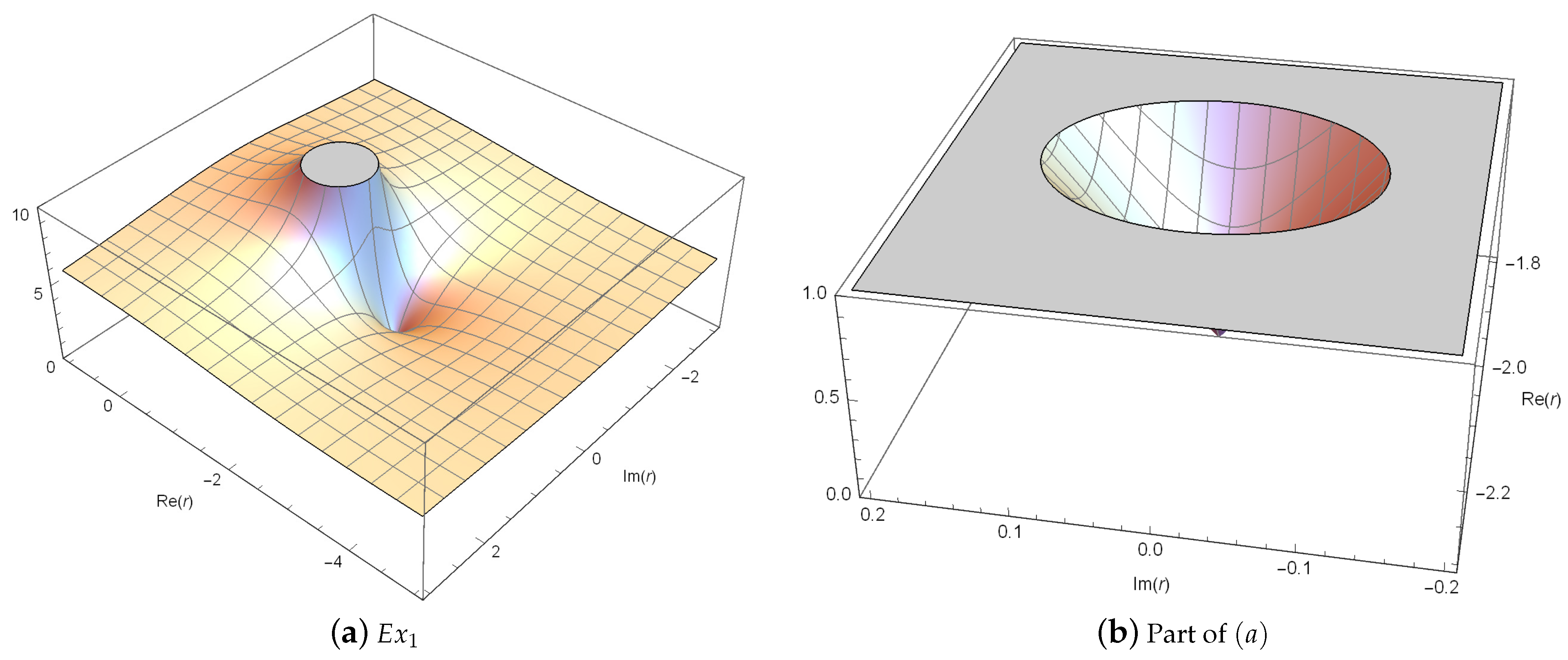
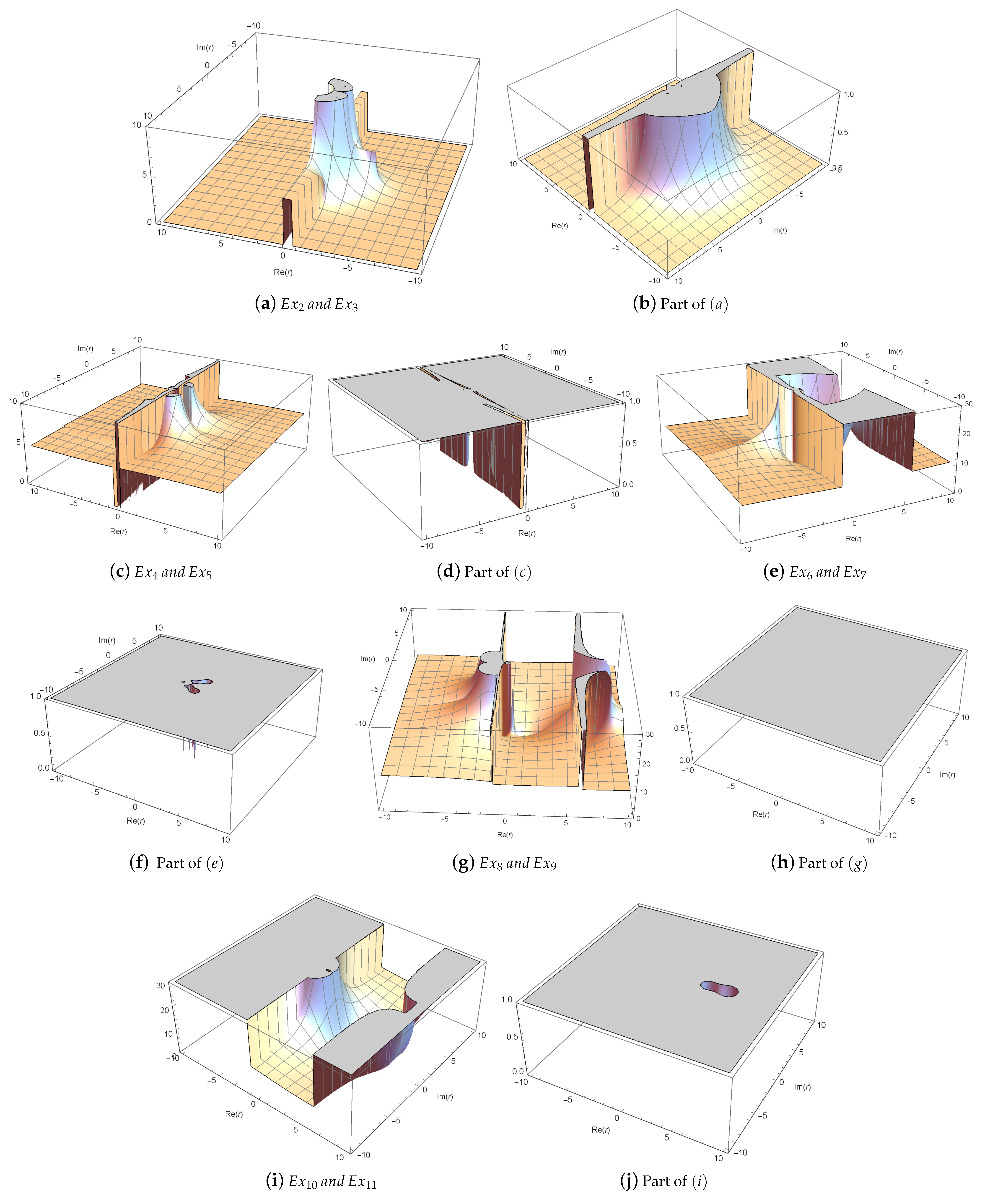
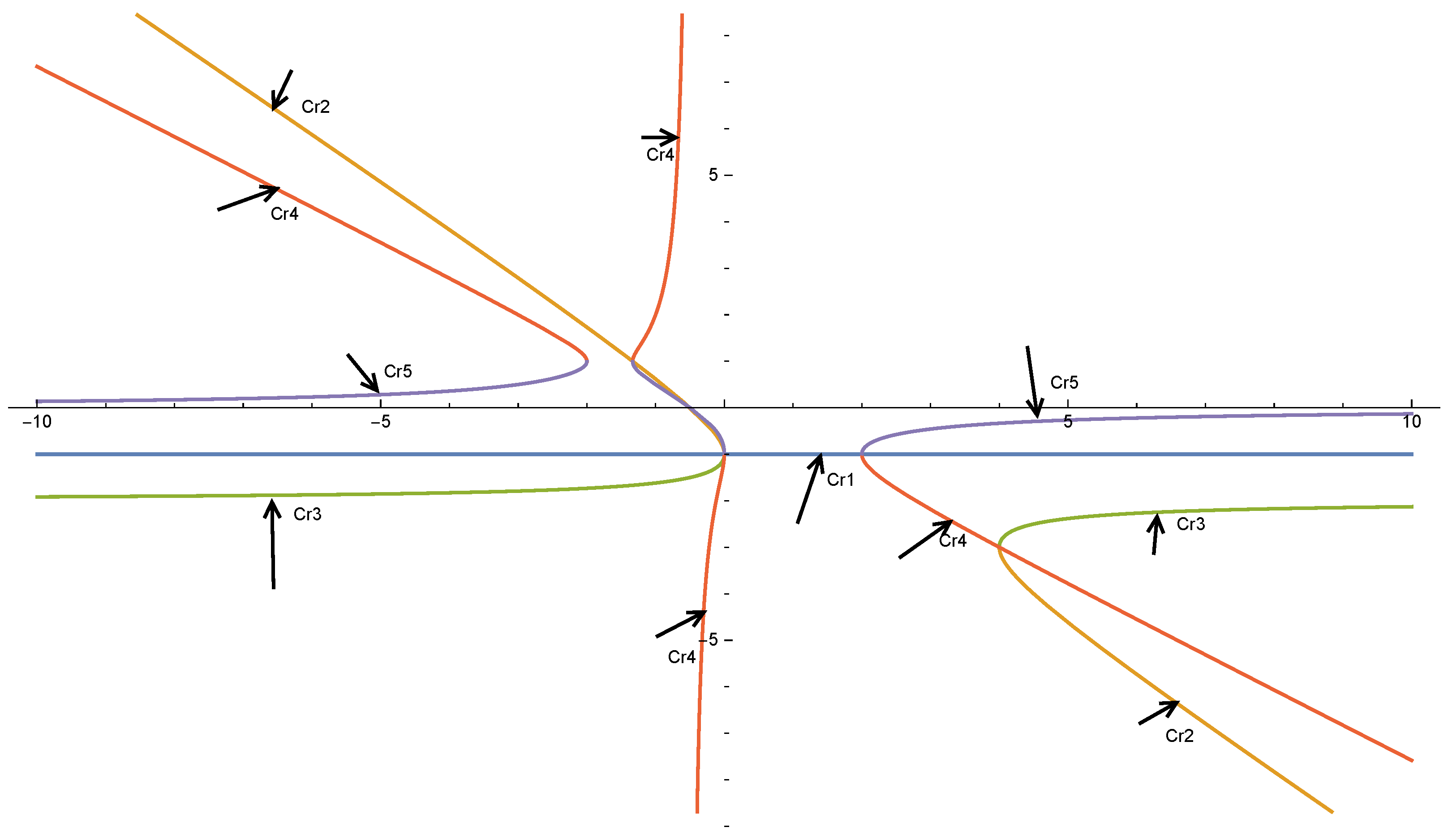
3.2. Analysis of Critical Points

The critical points of M ( z ; r ) can be obtained according to M ( z ; r ) = 0 in (7). z = 0 and z = are obviously the critical points related to the roots of f ( z ) = ( z a ) ( z b ) . The critical point unrelated to roots a , b is called the free critical point, and the free critical points are represented by C r i , respectively.
Corollary 3. 
If z is a critical point of M ( z ; r ) , then so is 1 z .
Proof. 
By Lemma 2, for a given r C and z C ˜ , we obtain
M ( z ; r ) · M ( 1 z ; r ) 1 z 2 M ( z ; r ) · M ( 1 z ; r ) = 0 .
Hence, if M ( z ; r ) = 0 , then M ( 1 z ; r ) = 0 . □
Theorem 6. 
The free critical points of M ( z ; r ) are:
  • C r 1 = 1 ;
  • C r 2 = 1 2 ( 2 4 + r r r ) ;
  • C r 3 = 1 2 ( 2 + 4 + r r r ) = 1 C r 2 ;
  • C r 4 = 4 2 r 3 r 2 3 16 r 12 r 2 + 4 r 3 + 3 r 4 4 ( 1 + 2 r ) ;
  • C r 5 = 4 2 r 3 r 2 + 3 16 r 12 r 2 + 4 r 3 + 3 r 4 4 ( 1 + 2 r ) = 1 C r 4 .
Figure 3 shows the bifurcation diagram of the critical point when r is real. From the image, the following conclusions are directly established:
Remark 1. 
For the critical point C r i , 1 i 5 , the following relationships hold:
  • Relation C r 2 = C r 3 holds when r = 0 or r = 4 ;
  • Relation C r 4 = C r 5 holds when r = 2 , r = 4 3 , r = 0 or r = 2 ;
  • Relation C r 2 = C r 4 holds when r = 4 3 , r = 0 or r = 4 ;
  • Relation C r 3 = C r 5 holds when r = 0 ;
  • Relation C r 1 = C r 2 = C r 3 = 1 holds when r = 0 ;
  • Relation C r 1 = C r 4 = C r 5 = 1 holds when r = 0 or r = 2 ;
  • Relation C r 2 = C r 3 = C r 4 = C r 5 holds when r = 0 .

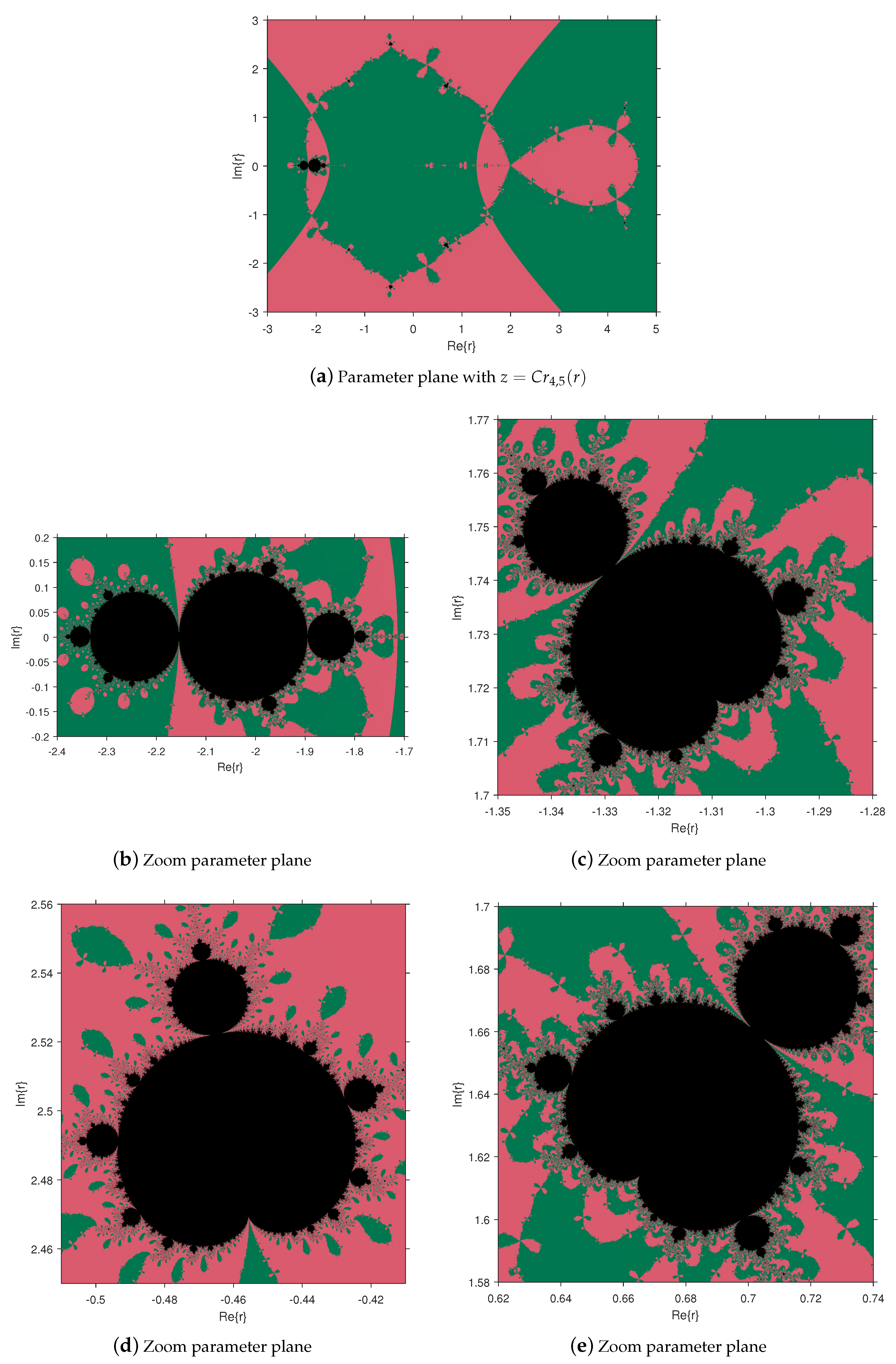
3.3. Parameter Spaces and Dynamical Planes

In this part, in order to describe the iterative mapping M ( z ; r ) , we use the parameter space P and the dynamical plane D . We draw the parameter space generated by the critical point as the initial point. By observing the parameter space, we can choose a stable parameter set; thus, we can avoid the selection of these unstable parameters. In addition, according to the determined parameters, the dynamical plane is drawn to observe the convergence of the iterative method (1). Finally, we determine the most stable parameters for an efficient solution to practical problems.
P = { r C : a n o r b i t o f a f r e e c r i t i c a l p o i n t z ( r ) t e n d s t o a n u m b e r ε p C ˜ u n d e r t h e a c t i o n o f M ( z ; r ) } ,
D = { z C : a n o r b i t o f z ( r ) f o r a g i v e n r P t e n d s t o a n u m b e r ε d C ˜ u n d e r t h e a c t i o n o f M ( z ; r ) } .

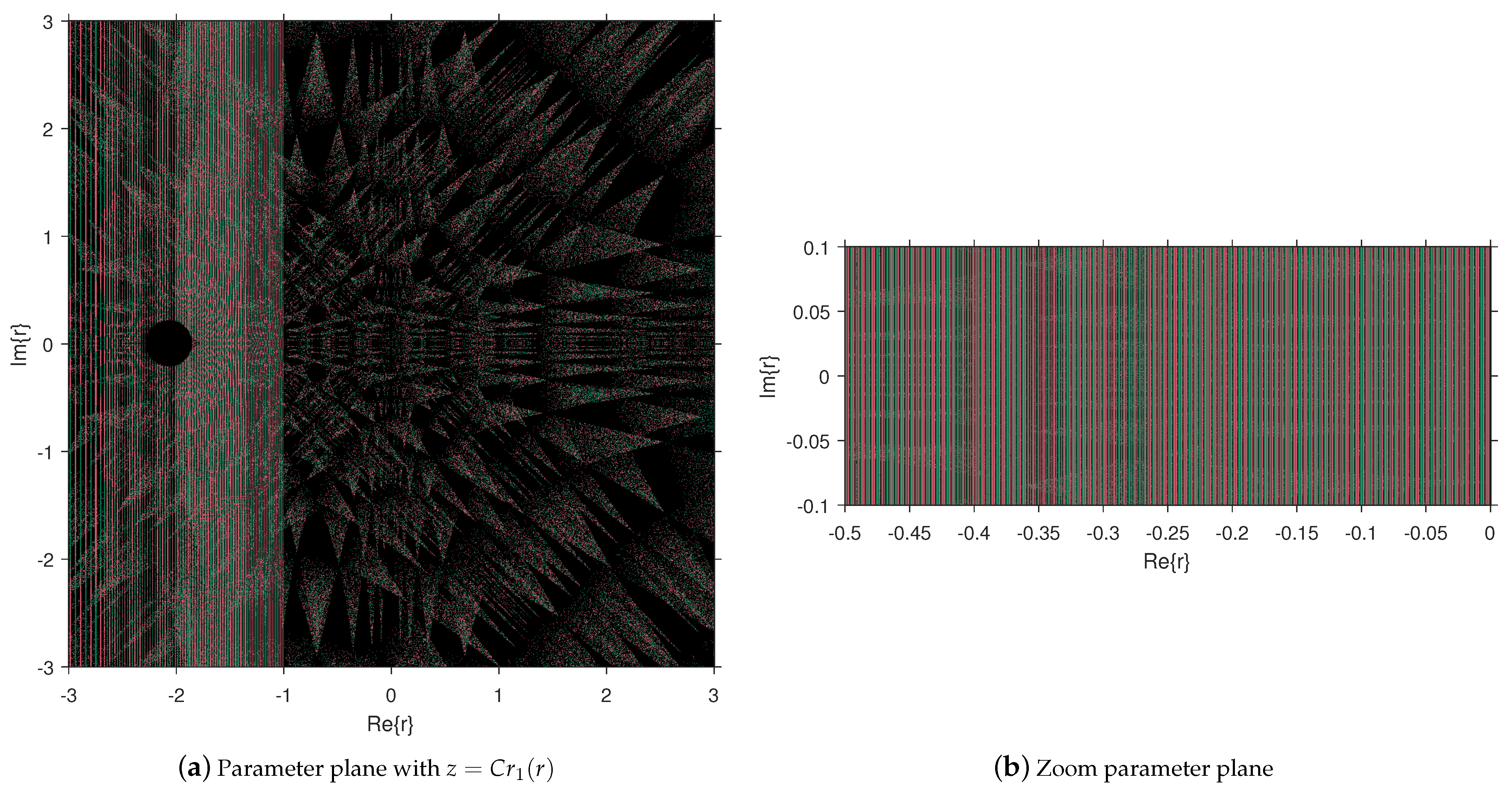
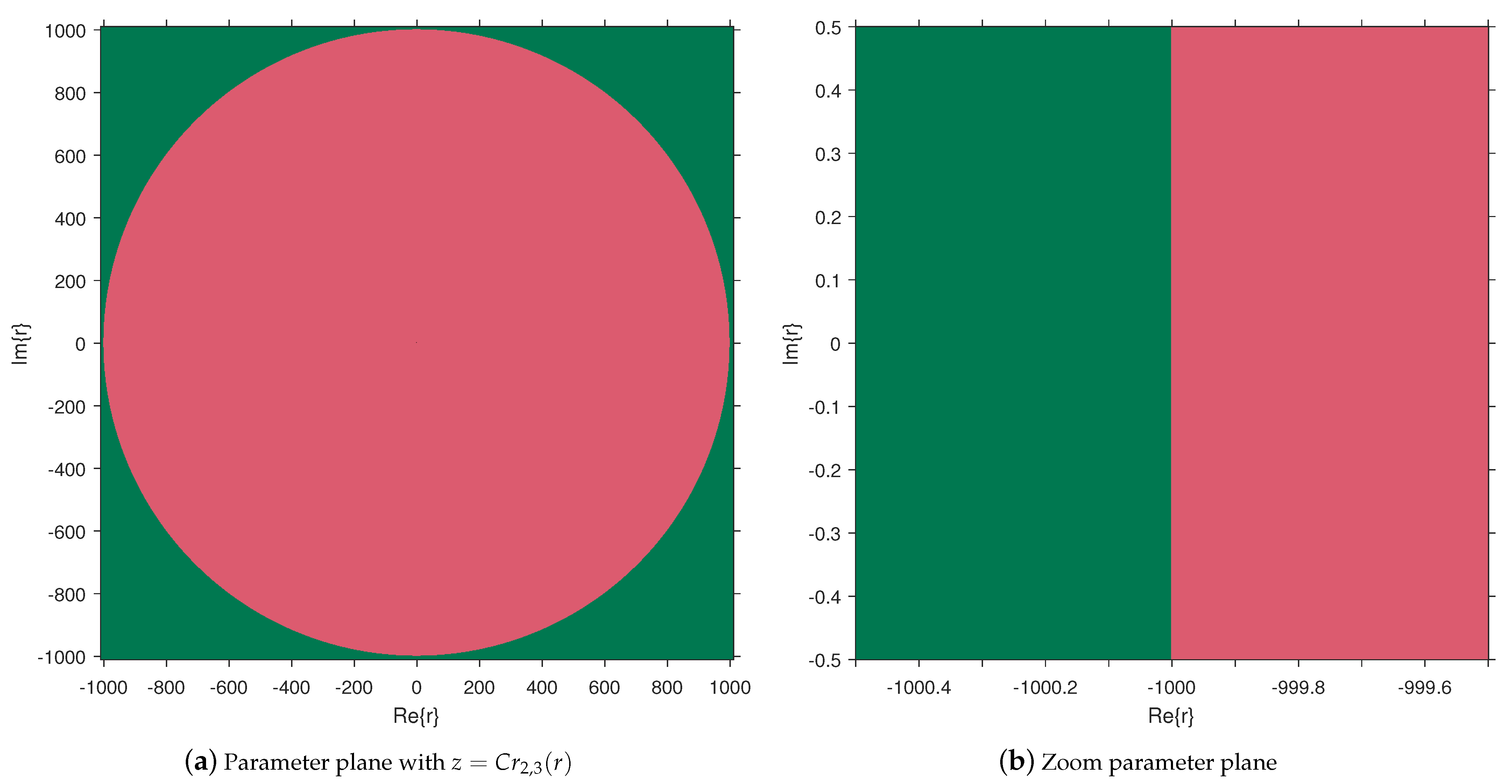
3.3.1. Parameter Spaces

We select a 1000 × 1000 plane point with a critical point as the starting point after a maximum of 80 iterations to generate parameter space. If the sequence converges to 0 during the iteration, it is represented in pink; if the sequence converges to , it is represented in green; and black represents other cases, including nonconvergence. Figure 4 shows the parameter space corresponding to the iteration sequence generated from the free critical point C r 1 = 1 , mostly black.
A similar process can be performed for the free critical points C r 2 , 3 and C r 4 , 5 , and the corresponding parameter spaces P 1 and P 2 can be obtained, as shown in Figure 5 and Figure 6. In Figure 5, there are only pink and green regions, indicating that the sequence generated from C r 2 , 3 always converges to the roots regardless of the parameter r. This situation is exactly what we expect, indicating that the corresponding iterative method is stable with C r 2 , 3 as the initial point. In Figure 6, the black area appears. By zooming the local areas, we observed a black pattern that has some similarity to the known Mandelbrot set [26]. In addition, the iterative method corresponding to the r value in the black region is unstable, for example, r = 2.2 , 1.8 , 0.45 + 2.5 i , 0.5 + 2.5 i , 0.73 + 1.7 i , because the sequence generated by the critical points C r 4 , 5 does not converge to the roots a and b. So, in the selection of r in (1), we try to avoid the values in the black area as much as possible and instead select the values in the green and pink areas.

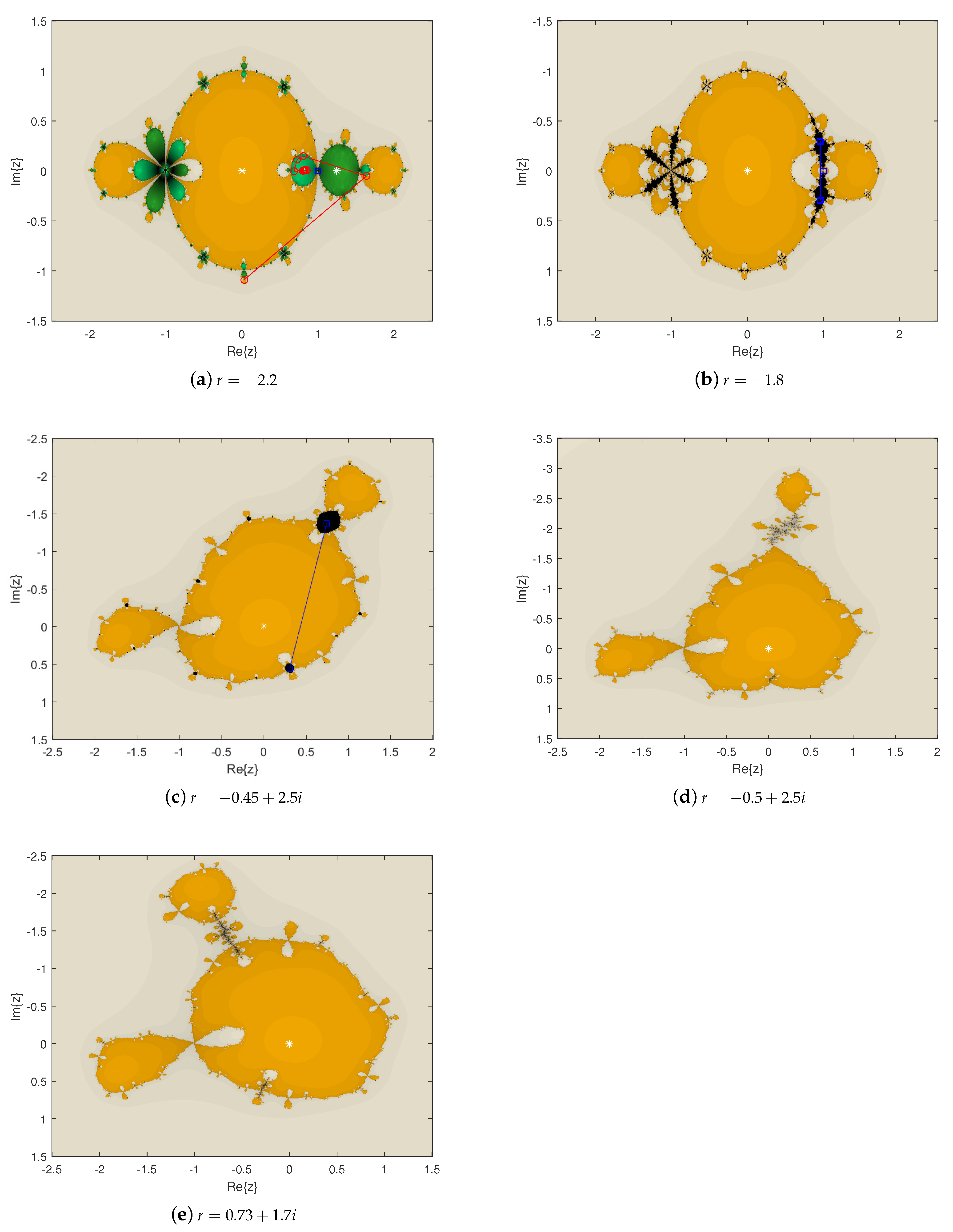
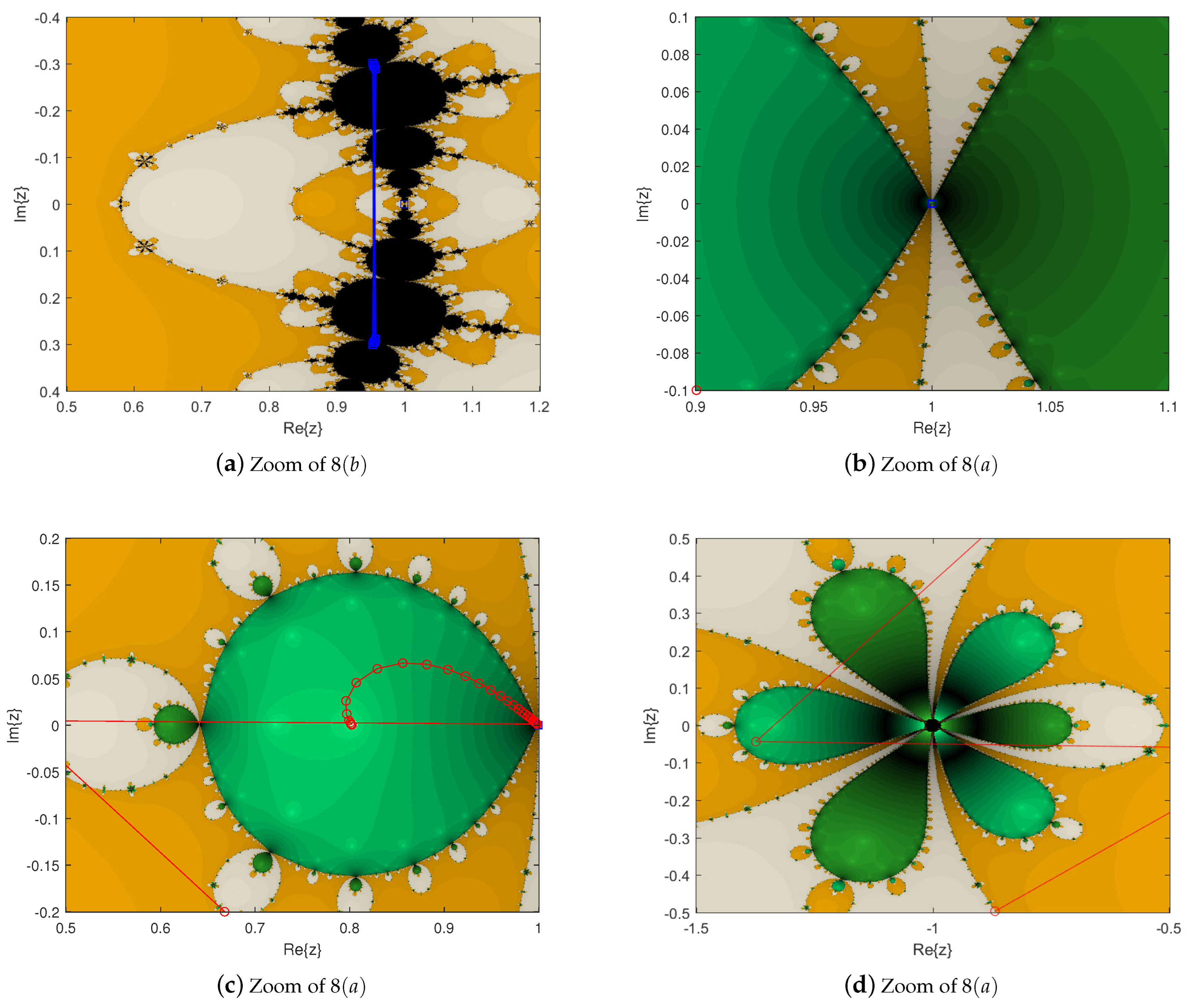
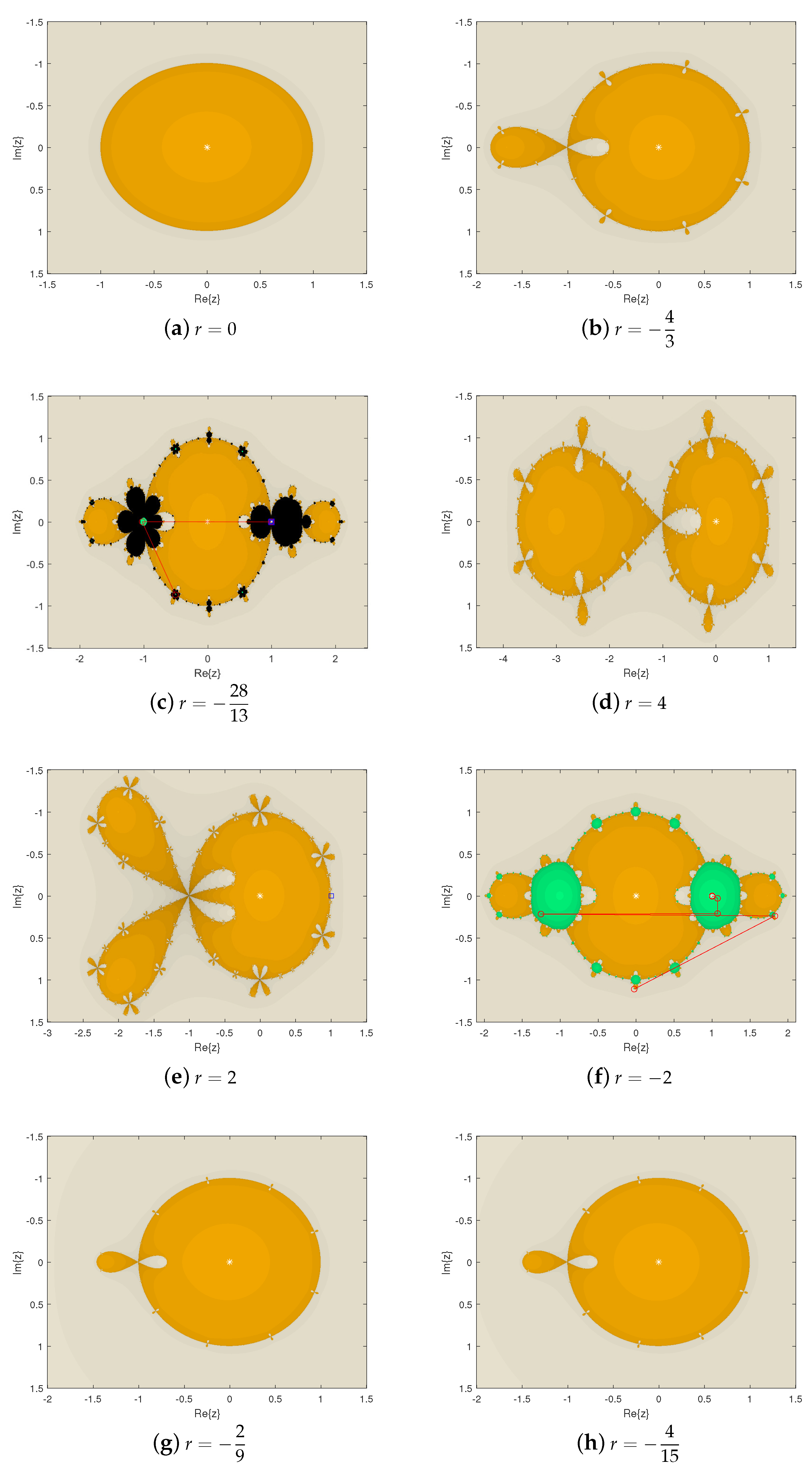
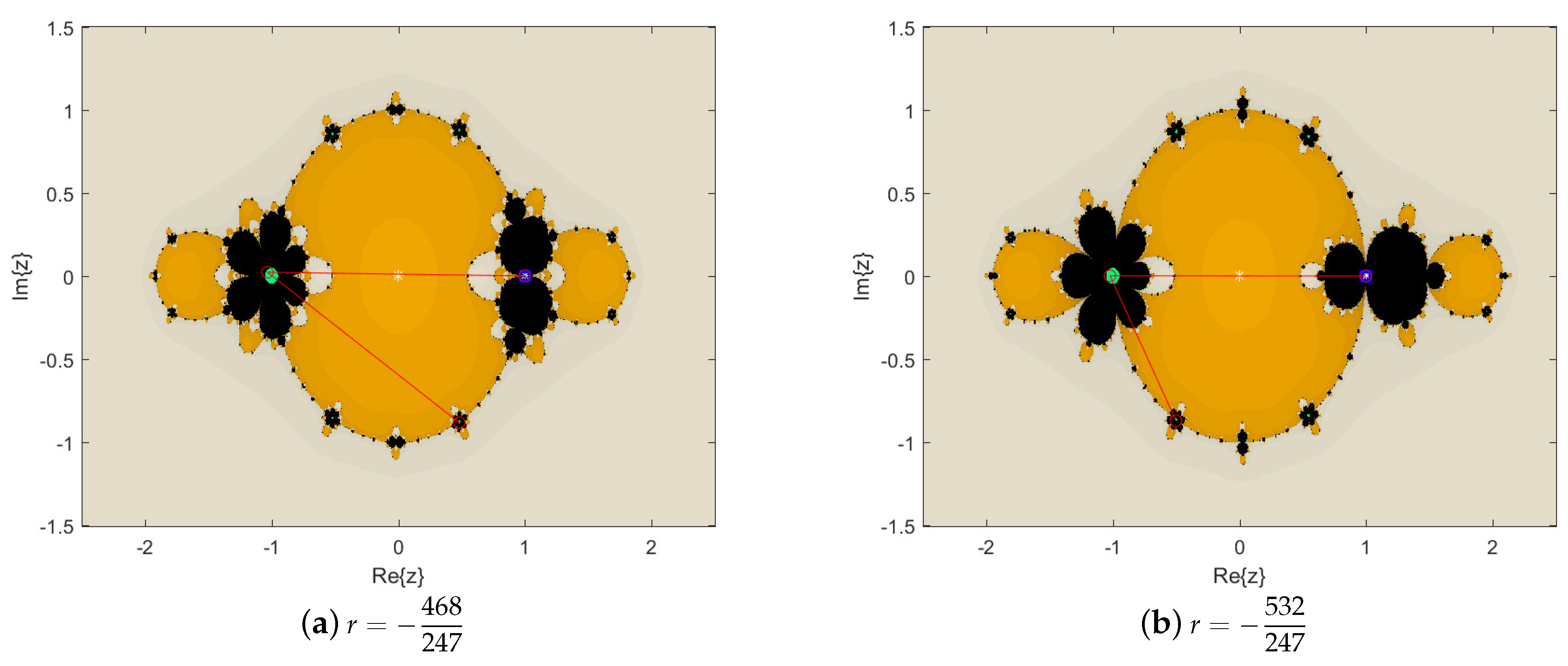
3.3.2. Dynamical Planes

By giving the parameter r, we perform up to 50 iterations on the grid points of 800 × 800 to draw a dynamical plane. If the iteration converges to 0, it is drawn yellow; if it converges to , it is represented in ivory. Peak green indicates that the iterative sequence converges to 1, and black indicates that it does not converge. We are interested in the parameter values without black regions. In addition, the white asterisk “∗” represents the attractive point, the blue square “⋄” represents the periodic point, the orbit of the periodic point is represented by blue, the red circle “∘” represents the additional fixed point and the convergence orbit is represented by red.
According to the above drawing specification, combined with the theorems and conclusions of the previous sections, we draw the dynamical plane of the iterative method (1) by the given parameter r, observe its dynamic behavior and analyze its stability.
The r value in Figure 7 is determined by Theorems 2 and 3. In Figure 7, only the black region appears in Figure 7c, indicating that the iterative method has nonconvergence behavior. Green regions appear in Figure 7c,f, suggesting that the corresponding iterative method converges to the fixed point E x 1 = 1 in addition to 0 and . The previous theorems and figures also illustrate this result. For example, by calculation, Theorem 4 ( d ) shows that z = 1 is a superattracting point at r = 2 . In Figure 1b, we observe the point at r = 2 , corresponding to the golden region, which means that when r = 2 , the iterative method (1) converges to the fixed point E x 1 = 1 in addition to the roots a and b, that is, the iterative method is unstable. In Figure 6e, the parameter space P 2 also presents a black area when r = 2 . In addition, we also note that the dynamical planes shown in Figure 7g,h are the same, indicating that the stability of the iterative methods corresponding to r = 2 9 and r = 4 15 is not much different, and both are stable. In fact, when considering the stability of the iterative methods with fixed points and critical points as the initial points, combined with Figure 1, Figure 2, Figure 4 and Figure 5, we can deduce that most of the iterative methods corresponding to the real value r in [ 0.5 , 0 ] × [ 0.1 , 0.1 ] are stable.
Figure 8 shows the dynamical plane by selecting the r value from the black region in the parameter space P 2 . The results show that there are indeed unstable behaviors in these cases. Figure 9 is a partial detail of them. Figure 10 shows the dynamical plane of the parameter r that makes the fixed point E x 1 = 1 neutral.
In Figure 7, Figure 8, Figure 9 and Figure 10, we notice that periodic points appear in Figure 7c,e, Figure 8a–c and Figure 10a,b, where the blue line represents the orbit of the periodic point. Figure 7c,f, Figure 8a and Figure 10a,b all show the behavior orbit of an extra fixed point with red lines, which come from E x 1 = 1 or the roots of N ( z ; r ) = 0 in (6). In addition, for the dynamic behavior diagrams with nonconvergence behavior in Figure 7c, Figure 8a–e and Figure 10a,b, in the dynamical plane diagram with the same range, the larger the black area is, the more unstable the dynamic behavior of the iterative method is. Based on the above description, it is shown that the parameters corresponding to these figures belong to the unstable parameter family.
By analyzing the dynamic behavior of (1) with different parameters, we obtain the stable parameter set r { 0 , 4 3 , 4 , 2 9 , 4 15 } and the unstable parameter set r { 28 13 , 2 , 2 , 2.2 , 1.8 , 0.45 + 2.5 i , 0.5 + 2.5 i , 0.73 + 1.7 i , 468 247 , 532 247 } , which facilitates the selection of parameters when solving nonlinear equations using the iterative method (1).

4. Conclusions

In this paper, the fractal behavior of a class of the optimal eighth-order single-parameter Petković family is studied. By regarding the number of iterations in the iterative method (1) as a time index, the process of solving the nonlinear equation f ( x ) = 0 for a given initial point x 0 can be regarded as an image sequence in a dynamic system. Under Möbius conjugate mapping, the connection between iterative method and rational operator makes it simple to explore the fractal behavior of the iterative method.
To start with, in the process of solving the fixed point and critical point of (5), some special parameter r values are found by analyzing the relationship between numerators and denominators in (6) and (7), respectively. Secondly, by analyzing the fixed points and critical points in turn, as well as their stability behavior, we also obtain the fixed point stability surface diagram and parameter space. We find the stability relationship between the parameter r and the initial point z 0 , that is, we select a parameter r C from the parameter space P , and the critical point related to P is used as the initial point of the iteration to determine whether the generated sequence converges to the fixed point, which corresponds to the fixed point stable surface diagram, as shown in Figure 1, Figure 2 and Figure 4, Figure 5 and Figure 6. In addition, by drawing the dynamic behavior diagram of the given parameters, the previous theorems and conclusions are verified; see Figure 7, Figure 8, Figure 9 and Figure 10. Conclusively, we attain the member choice with good dynamic behavior in the optimal eighth-order Petković family (1), that is, r { 0 , 4 3 , 4 , 2 , 2 9 , 4 15 } . Furthermore, we conclude from Figure 7a that r = 0 is the most stable parameter.

Author Contributions

Methodology, X.W.; writing—original draft preparation, W.L. All authors have read and agreed to the published version of the manuscript.

Funding

This research was supported by the National Natural Science Foundation of China (No. 61976027), the National Natural Science Foundation of Liaoning Province (No. 2022-MS-371), Educational Commission Foundation of Liaoning Province of China (Nos. LJKMZ20221492, LJKMZ20221498) and the Key Project of Bohai University (No. 0522xn078).

Data Availability Statement

Not applicable.

Conflicts of Interest

The authors declare no conflict of interest.

References

  1. Mandelbrot, B.B.; Aizenman, M. Fractals: Form, Chance, and Dimension. Phys. Today 1979, 32, 65–66. [Google Scholar] [CrossRef]
  2. Agop, M.; Gavriluţ, A.; Pǎun, V.P. Fractal Information by Means of Harmonic Mappings and some Physical Implications. Entropy 2016, 18, 160. [Google Scholar] [CrossRef]
  3. Zhong, X.; Zhu, Y.; Zhou, Y. Spectra of fractal information on Cantor axis. Phys. A 1993, 1711, 349–356. [Google Scholar]
  4. Shailendra, K.D.; Umesh, D.; Sanyog, R. A Slotted Microstrip Antenna with Fractal Design for Surveillance Based Radar Applications in X-band. Int. J. Eng. Sci. 2018, 7, 64. [Google Scholar]
  5. Qu, H.; Han, Z.; Chen, Z. Fractal Design Boosts Extrusion-Based 3D Printing of Bone-Mimicking Radial-Gradient Scaffolds. Research 2021, 2021, 9892689. [Google Scholar] [CrossRef]
  6. Lin, X.; Liu, W. The Application of Fractal Art in Ceramic Product Design. IOP Conf. Ser. Mater. Sci. Eng. 2019, 573, 012003. [Google Scholar] [CrossRef]
  7. Kumari, S.; Gdawiec, K.; Nandal, A.; Postolache, M.; Chugh, R. A novel approach to generate Mandelbrot sets, Julia sets and biomorphs via viscosity approximation method. Chaos Solitons Fractals 2022, 163, 112540. [Google Scholar] [CrossRef]
  8. Usurelu, G.I.; Bejenaru, A.; Postolache, M. Newton-like methods and polynomiographic visualization of modified Thakur processes. Int. J. Comput. Math. 2021, 98, 1049–1068. [Google Scholar] [CrossRef]
  9. Zhang, T.; Guo, Q. The solution theory of the nonlinear q-fractional differential equations. Appl. Math. Lett. 2020, 104, 106282. [Google Scholar] [CrossRef]
  10. Ryu, K.; Yücesan, E.; Jung, M. Dynamic restructuring process for self-reconfiguration in the fractal manufacturing system. Int. J. Prod. Res. 2011, 44, 3105–3129. [Google Scholar] [CrossRef]
  11. Yorikawa, H. Energy levels in a self-similar fractal cluster. J. Phys. Commun. 2019, 3, 085004. [Google Scholar] [CrossRef]
  12. Alexander, T.; Trifce, S. Fractional Diffusion to a Cantor Set in 2D. Fractal Fract. 2020, 4, 52. [Google Scholar]
  13. Paramanathan, P.; Uthayakumar, R. Fractal interpolation on the Koch Curve. Comput. Math. Appl. 2010, 59, 3229–3233. [Google Scholar] [CrossRef]
  14. Bock, H. On the dynamics of entire functions on the Julia set. Results Math. 1996, 30, 16–20. [Google Scholar] [CrossRef]
  15. Peitgen, H.; Richter, P. The Beauty of Fractals; Springer: New York, NY, USA, 1986. [Google Scholar]
  16. Letherman, S.D.; Wood, R.M.W. A note on the Julia set of a rational function. Math. Proc. Camb. Philos. Soc. 1995, 118, 477–485. [Google Scholar] [CrossRef]
  17. Hua, X.; Yang, C.C. Fatou Components and a Problem of Bergweiler. Int. J. Bifurc. Chaos Appl. Sci. Eng. 1998, 8, 1613–1616. [Google Scholar] [CrossRef]
  18. Wang, X.; Chen, X. Derivative-Free Kurchatov-Type Accelerating Iterative Method for Solving Nonlinear Systems: Dynamics and Applications. Fractal Fract. 2022, 6, 59. [Google Scholar] [CrossRef]
  19. Geum, Y.H.; Kim, Y.I. Computational Bifurcations Occurring on Red Fixed Components in the λ-Parameter Plane for a Family of Optimal Fourth-Order Multiple-Root Finders under the Möbius Conjugacy Map. Mathematics 2020, 8, 763. [Google Scholar] [CrossRef]
  20. Geum, Y.H.; Kim, Y.I.; Magreñán, Á.A. A biparametric extension of King’s fourth-order methods and their dynamics. Appl. Math Comput. 2016, 282, 254–275. [Google Scholar] [CrossRef]
  21. Petković, M.S.; Petković, L.D. Families of optimal multipoint methods for solving nonlinear equations: A survey. Appl. Anal. Discr. Math. 2010, 4, 1–22. [Google Scholar] [CrossRef]
  22. Campos, B.; Cordero, A.; Torregrosa, J.R.; Vindel, P. Orbits of period two in the family of a multipoint variant of Chebyshev-Halley family. Numer. Algorithms 2016, 73, 141–156. [Google Scholar] [CrossRef] [Green Version]
  23. Lee, M.; Kim, Y.I. The dynamical analysis of a uniparametric family of three-point optimal eighth-order multiple-root finders under the Möbius conjugacy map on the Riemann sphere. Numer. Algorithms 2020, 83, 1063–1090. [Google Scholar] [CrossRef]
  24. Russen, S.C. Nonlinear dynamics and chaos. Math. Gaz. 2004, 88, 188. [Google Scholar] [CrossRef]
  25. Takens, F. An introduction to chaotic dynamical systems. Acta Appl. Math. 1988, 13, 221–226. [Google Scholar] [CrossRef]
  26. Devaney, R.L. The Mandelbrot set, the Farey tree and the Fibonacci sequence. Am. Math. Mon. 1999, 106, 289–302. [Google Scholar] [CrossRef]
Figure 1. Stability surfaces of E x 1 = 1 .
Fractalfract 06 00749 g001
Figure 2. Stability surfaces of the other ten strange fixed points.
Fractalfract 06 00749 g002
Figure 3. Bifurcation diagram of critical points.
Fractalfract 06 00749 g003
Figure 4. Parameter spaces for free critical points C r 1 = 1 .
Fractalfract 06 00749 g004
Figure 5. P 1 for C r 2 , 3 .
Fractalfract 06 00749 g005
Figure 6. P 2 for C r 4 , 5 .
Fractalfract 06 00749 g006
Figure 7. Dynamical planes of special r-values.
Fractalfract 06 00749 g007
Figure 8. Dynamical planes of special r-values.
Fractalfract 06 00749 g008
Figure 9. Local detail of Figure 8.
Fractalfract 06 00749 g009
Figure 10. Dynamical plane of parameters that make E x 1 a neutral point.
Fractalfract 06 00749 g010
Publisher’s Note: MDPI stays neutral with regard to jurisdictional claims in published maps and institutional affiliations.

