Investigation of the Ripa Model via NHRS Scheme with Its Wide-Ranging Applications

Abstract

This paper presents numerical modeling and investigation for the Ripa system. This model is derived from a shallow water model by merging the horizontal temperature gradients. We applied the non-homogeneous Riemann solver (NHRS) method for solving the Ripa model. This scheme contains two stages named predictor and corrector. The first one is made up of a control parameter that is responsible for the numerical diffusion. The second one recuperates the balance conservation equation. One of the main features of the NHRS scheme, it can determine the numerical flux corresponding to the real state of solution in the non-attendance of Riemann solution. Various test cases of physical interest are considered. These case studies display the high resolution of the NHRS scheme and emphasize its ability to produce accurate results for the Ripa model. The presented solutions are very critical in superfluid applications of energy and many others. Finally, the NHRS technique can be used to solve a wide range of additional models in applied research.

1. Introduction

Tsunami and ocean acoustic wave fields were generated by tremors along Japan’s coast in 2011, most of which were connected to short-distance seismic events [1]. In reality, Chunga and Toulkeridis’ research [2] introduced the first signs of natural disasters, where the seismic sea waves’ wavelength range and height are particularly noteworthy. Because of the widespread use of electrical devices and the large consumption of electricity, it is vital to increase the efficiency of this equipment. So, the study of models reflecting the oceanic phenomena is vital and has powerful applications. Various oceanic phenomena can be studied utilizing layered systems, where the continuous vertical structure is approximated by a small stack of layers with changing thicknesses [3]. The variables in each layer, such as horizontal velocity and density, are considered as vertically uniform. The shallow water system is the simplest layer example for a single layer of incompressible fluid via a free surface [3,4,5]. Ripa [6] studied a family of layered systems, which allowed horizontal variations in the fluid density in each layer. The Ripa system is generalized from the shallow water model. The Ripa system of nonlinear hyperbolic equations was investigated to examine the attitude of ocean currents, see [6,7,8]. Time delay has become a highly crucial aspect in hyperbolic systems of conservation laws to produce more precise and objective outcomes. There are many studies of conservation laws in which the velocity depends nonlocally on the solution, not in real time but in a time-delayed manner [9]. A time-delay system for fluid flow networks was developed by the authors of [10], which resulted in a traditional state–space representation with delays to take network transport phenomena into consideration. The authors in [10] considered analytical and numerical features of the Lighthill–Whitham–Richards traffic flow model though time delay.

The one-dimensional (1D) Ripa equations are given as follows:

$$\begin{array}{c}{\left(h\right)}_t+{\left(hu\right)}_x=0,\hfill \\ {\left(hu\right)}_t+{(h{u}^2+\frac{g{h}^2\theta }{2})}_x=-gh\theta Z_x,\hfill \\ {\left(h\theta \right)}_t+{\left(hu\theta \right)}_x=0\hfill \end{array}$$

(1)

where h is free surface elevation, u is the x-component of velocity, $Z\left(x\right)$ denotes the bottom topograph, g is the gravity constant, and $\theta >$ 0 is the temperature. The term $hu$ denotes water discharge, $h+Z$ denotes the water surface, and $\frac{g{h}^2\theta }{2}$ denotes the pressure relying on the water temperature of liquid.

The 1D shallow water equations are given as follows:

$$\begin{array}{c}{\left(h\right)}_t+{\left(hu\right)}_x=0,\hfill \\ {\left(hu\right)}_t+{(h{u}^2+\frac{g{h}^2\theta }{2})}_x=-gh\theta Z_x.\hfill \end{array}$$

(2)

At $\theta =1$, the Ripa system becomes the 1D shallow water model (2), which includes conservation of mass and momentum for constant density. Due to the presence of a source term that accounts for bottom fluctuation, the Ripa model (1) cannot be expressed in conservative form. This source term presents various troubles in investigating the model numerically or analytically, and classical techniques failed. Recently, various numerical schemes have been presented in the presence of the source term in a shallow water model with non-flat bottom topographies [11,12,13].

The Ripa and shallow water systems (1) and (2) are hyperbolic balance laws that have attracted more attention in recent years. These models take the following form:

$$W_t+F{\left(W\right)}_x=Q\left(W\right).$$

(3)

As a result of the presence of the source term $Q\left(W\right)$, hyperbolic balance laws present vital computational challenges. This balance, the source term, and small perturbations of steady state solutions cannot be handled by common numerical techniques, except if a much refined mesh is utilized.

The steady state solutions for Equation (1) happen for $W_t=0$, i.e.,

$$\begin{array}{c}{\left(hu\right)}_x=0,\hfill \\ {(h{u}^2+\frac{g{h}^2\theta }{2})}_x=-gh\theta Z_x,\hfill \\ {\left(hu\theta \right)}_x=0.\hfill \end{array}$$

(4)

In the case of still water (states at rest at $u=0$), the steady state Equation (4) becomes

$$\begin{array}{c}u=0,\hfill \\ {(\frac{h^2\theta }{2})}_x+h\theta Z_x=0.\hfill \end{array}$$

(5)

The main contradiction between the shallow water and Ripa systems is due to the steady states at rest. It is impossible to integrate the system (5), and no general steady states can be explicitly given. In order to solve this system, extra hypotheses for $h, \theta orB$ must be imposed. These certain steady states at rest are physically relevant [14,15]:

Case 1: Still-water steady state

This case identifies a flat water surface via constant temperature:

$$(u,\theta ,h+Z)=(0,C_1,C_2).$$

(6)

Case 2: Isobaric steady state

This case identifies a wave where the height and temperature jump but pressure and velocity stay constant:

$$(u,Z,h^2\theta )=(0,C_1,C_2).$$

(7)

Case 3: Constant water height steady state:

$$(u,h,Z+\frac{h}{2}ln\theta )=(0,C_1,C_2).$$

(8)

Here, $C_1$ and $C_2$ are constants.

The more general case happens for $u\ne 0$. The moving-water equilibrium is [15]:

$$\begin{array}{c}hu=const,\hfill \\ \theta =const,\hfill \\ \frac{u^2}{2}+g\theta (h+Z)=const,\hfill \end{array}$$

(9)

the momentum and potential temperature field, $hu$, $\theta$, respectively, are constant. Notice that Case 1 is a special case of the moving-water steady state (9). Actually, the principle of conservation of mass, momentum, and energy are utilized to produce the Rankine–Hugoniot conditions near the bottom discontinuity [16]. With the aid of the interface tracking approach [17], Chertock et al. [18] provide a well-balanced central-upwind scheme for the 1D and 2D Ripa model. Furthermore, Desveaux et al. [14] develop a well-balanced relaxation technique for the 1D Ripa system. Touma et al. [19] investigate the 1D Ripa system within the context of central schemes. In recent years, various numerical techniques were proposed to solve the Ripa system and their steady states, see for example [20,21,22,23,24,25,26,27].

The main aspect of this article is to develop a non-homogeneous Riemann solver (NHRS) to solve the Ripa model. This scheme contains two stages, namely, predictor and corrector stages [28,29,30,31,32,33]. The first one includes a parameter of control to numerical diffusion that is modulated by utilizing Riemann invariants and limiters theory. The second stage recovers the balance conservation equation. The numerical flux was calculated by using Riemann solutions in the majority of typical schemes. The NHRS scheme, in contrast to previous schemes, has the intriguing ability to compute the numerical flux in the nonappearance of the Riemann solution. Actually, this method can be used as a box solver for a wide variety of other conservation law models. We introduce numerous numerical examples for the Ripa system with flat bottom and with non-flat bottom to clarify the performance of the NHRS scheme. The numerical solutions obtained are compared to the Lax–Friedrichs approach, the Rusanov method, and the analytical solution. Our results show that the NHRS technique is a quit powerful approach. The stability analysis shows that the NHRS method is of Order 1 or 2 due to the value of the parameter of control, see [34].

This work is arranged as follows. Section 2 provides the main notions of the Ripa model with non-flat bottom and with flat bottom. Section 3 gives the NHRS scheme to solve the Ripa model. Numerical test cases using the NHRS scheme, the Rusanov scheme and the Lax–Friedrichs scheme are performed in Section 4. The conclusions are given in Section 5.

2. Mathematical Models

2.1. The 1D Ripa System for Flat Bottom

This section considers the Ripa model with flat bottom topography given as follows [16,35]:

$$\begin{array}{c}{\left(h\right)}_t+{\left(hu\right)}_x=0,\hfill \\ {\left(hu\right)}_t+{(h{u}^2+\frac{g{h}^2\theta }{2})}_x=0,\hfill \\ {\left(h\theta \right)}_t+{\left(hu\theta \right)}_x=0.\hfill \end{array}$$

(10)

Here, $h(x,t)$ is free surface elevation, $u(x,t)$ is the x-component of velocity, $Z\left(x\right)$ denotes the bottom topograph, g is the gravity constant, and $\theta >$ 0 is the temperature. Equation (10) can be rewritten as

$$W_t+F{\left(W\right)}_x=0,$$

(11)

where

$$W=\left(\begin{array}{c}{W}_1\\ W_2\\ W_3\end{array}\right)=\left(\begin{array}{c}h\\ hu\\ h\theta \end{array}\right),$$

$$F\left(W\right)=\left(\begin{array}{c}{W}_2\\ \frac{W_2^2}{W_1}+\frac{g}{2}{W}_1{W}_3\\ \frac{W_2{W}_3}{W_1}\end{array}\right).$$

For the calculation of the eigenvalues, we rewrite system (10) in the quasilinear form

$$W_t+A\left(W\right)W_x=0,$$

(12)

$A\left(W\right)$ is a Jacobian matrix given by

$$A\left(W\right)=\left(\begin{array}{ccc}0& 1& 0\\ -\frac{W_2^2}{W_1^2}+\frac{g{W}_3}{2}& 2\frac{W_2}{W_1}& \frac{g{W}_1}{2}\\ -\frac{W_2{W}_3}{W_1^2}& \frac{W_3}{W_1}& \frac{W_2}{W_1}\end{array}\right)=\left(\begin{array}{ccc}0& 1& 0\\ -u^2+\frac{gh\theta }{2}& 2u& \frac{gh}{2}\\ -u\theta & \theta & u\end{array}\right).$$

The system (10) has characteristic fields

$${\lambda }_1=u-a<{\lambda }_2=u<{\lambda }_3=u+a.$$

(13)

The corresponding eigenvectors of system (10) are

$$r_1={\left(1,u-a,\theta \right)}^T;r_2={\left(1,u,-\theta \right)}^T{r}_3={\left(1,u+a,\theta \right)}^T.$$

(14)

Proposition 1.

System (11) is strictly hyperbolic at $(h,u,\theta )$, where $h,\theta >0$ and $u\in \mathbb{R}$. The first and third eigenvalues are genuinely nonlinear, whereas the second eigenvalue is linearly degenerate.

Proof. 

The eigenvalues (13) show that Equation (10) is strictly hyperbolic. Indeed,

$$\begin{array}{c}{\displaystyle \nabla {\lambda }_1·r_1=\frac{-a}{h}-0.5\sqrt{\frac{g\theta }{h}}\ne 0,}\hfill \\ {\displaystyle \nabla {\lambda }_2·r_2=0,}\hfill \\ {\displaystyle \nabla {\lambda }_3·r_3=\frac{a}{h}+0.5\sqrt{\frac{g\theta }{h}}\ne 0,}\hfill \end{array}$$

(15)

which shows genuine nonlinearity for the first and third characteristic fields and the linearly degenerate of the second characteristic field. □

The characteristic fields ${\lambda }_1$ and ${\lambda }_3$ refer to the first and third family of waves (shock wave or a rarefaction wave (fan)), respectively. The second central wave (contact wave) lies between the other two waves, which correspond to the characteristic field ${\lambda }_2$. These waves construct four regions that are shown in Figure 1, where $W_{-}=(h_{-},u_{-},{\theta }_{-})$ is the left state, $W_{+}=(h_{+},u_{+},{\theta }_{+})$ is the right state, and $W_{-}^{*}=(h_{-}^{*},u_{-}^{*},{\theta }_{-}^{*})$ are the unknown left and right state, respectively, to the contact wave. For more details about the parametrization of elementary waves, namely, shock waves, contact waves, fans, and Riemann invariants, we refer to [16,35].

2.2. The 1D Ripa System with Non-Flat Bottom

For the sake of completeness of this article, we present some properties for the Ripa system (1). Because the topography function Z is independent of time,

$$Z_t=0.$$

Hence, we rewrite the Ripa model (1) in the following equivalent form:

$$\begin{array}{c}{\left(h\right)}_t+{\left(hu\right)}_x=0,\hfill \\ {\left(hu\right)}_t+{(h{u}^2+\frac{g{h}^2\theta }{2})}_x=-gh\theta Z_x,\hfill \\ {\left(h\theta \right)}_t+{\left(hu\theta \right)}_x=0,\hfill \\ Z_t=0.\hfill \end{array}$$

(16)

The model (16) is rewritten in a compact form of Equation (11), where

$$W=\left(\begin{array}{c}{W}_1\\ W_2\\ W_3\\ W_4\end{array}\right)=\left(\begin{array}{c}h\\ hu\\ h\theta \\ Z\end{array}\right),$$

$$F\left(W\right)=\left(\begin{array}{c}{W}_2\\ \frac{W_2^2}{W_1}+\frac{g}{2}{W}_1{W}_3\\ \frac{W_2{W}_3}{W_1}\\ 0\end{array}\right),$$

$$Q\left(W\right)=\left(\begin{array}{c}0\\ -g{W}_3\theta Z_x\\ 0\\ 0\end{array}\right).$$

For the calculation of the eigenvalues, we rewrite the $3\times 3$ system (16) in the quasilinear form

$$W_t+A\left(W\right)W_x=0,$$

(17)

$A\left(W\right)$ is a Jacobian matrix:

$$A\left(W\right)=\left(\begin{array}{cccc}0& 1& 0& 0\\ -\frac{W_2^2}{W_1^2}+\frac{g{W}_3}{2}& 2\frac{W_2}{W_1}& \frac{g{W}_1}{2}& g{W}_3\\ -\frac{W_2{W}_3}{W_1^2}& \frac{W_3}{W_1}& \frac{W_2}{W_1}& 0\\ 0& 0& 0& 0\end{array}\right)=\left(\begin{array}{cccc}0& 1& 0& 0\\ -u^2+\frac{gh\theta }{2}& 2u& \frac{gh}{2}& gh\theta \\ -u\theta & \theta & u& 0\\ 0& 0& 0& 0\end{array}\right).$$

The system (16) has eigenvalues

$${\lambda }_1=u-a,{\lambda }_2=u{\lambda }_3=u+a,{\lambda }_4=0.$$

(18)

The corresponding right-eigenvectors of model (16) are

$$r_1={\left(1,u-a,\theta ,0\right)}^T,r_2={\left(1,u,-\theta ,0\right)}^T,r_3={\left(1,u+a,\theta ,0\right)}^T,r_4={\left(-a,0,-a\theta ,u^2-gh\theta \right)}^T.$$

(19)

Proposition 2.

The first and third eigenvalues are genuinely nonlinear, and the second and fourth eigenvalues are linearly degenerate.

Proof. 

The results are clear because

$$\begin{array}{c}{\displaystyle \nabla {\lambda }_1·r_1=\frac{-a}{h}-0.5\sqrt{\frac{g\theta }{h}}\ne 0,}\hfill \\ {\displaystyle \nabla {\lambda }_2·r_2=0,}\hfill \\ {\displaystyle \nabla {\lambda }_3·r_3=\frac{a}{h}+0.5\sqrt{\frac{g\theta }{h}}\ne 0.}\hfill \\ {\displaystyle \nabla {\lambda }_4·r_4=0.}\hfill \end{array}$$

(20)

□

The characteristic fields ${\lambda }_1$ and ${\lambda }_3$ refer to the first and third family of waves (shock wave or fan), respectively. The third wave (contact wave) islocated between the shock wave and fans, which corresponds to the characteristic field ${\lambda }_2$. The fourth wave is named the stationary shock wave situated at $x_0$. These waves construct five regions that are depicted in Figure 2, where $W_{-}=(h_{-},u_{-},{\theta }_{-})$ is a left state; $W_{+}=(h_{+},u_{+},{\theta }_{+})$ is a right state; $W_{-}^{*}=(h_{-}^{*},u_{-}^{*},{\theta }_{-}^{*})$ is a left state to the stationary shock wave; and $W_{+}^{*}=(h_{+}^{*},u_{+}^{*},{\theta }_{+}^{*})$ & $W^{*}=(h^{*},u^{*},{\theta }^{*})$ are the unknown left and right state, respectively, to the contact wave. For more details about the parametrization of shock waves, contact waves, stationary shock wave, fans, and Riemann invariants, we refer to [16,35].

3. The NHRS Scheme

To deduce the NHRS scheme, we integrate Equation (3) through the domain $[t_n,t_{n+1}]\times [x_{i-\frac{1}{2}},x_{i+\frac{1}{2}}]$. We obtain the following formula

$$W_i^{n+1}=W_i^n-\frac{\Delta t}{\Delta x}\left(F\left(W_{i+\frac{1}{2}}^n\right)-F\left(W_{i-\frac{1}{2}}^n\right)\right)+\Delta t_n{Q}_i^n,$$

(21)

where $W_i^n$ is the space-time of the solution W, ${\displaystyle Q_i^n}$ is the approximation of ${\displaystyle \frac{1}{\Delta t_n\Delta x}\underset{R}{\int }Q\left(x,W\right)}$$dxdt$, and $F\left(W_{i\pm \frac{1}{2}}^n\right)$ is the numerical flux at the interface $x=x_{i\pm \frac{1}{2}}$ and time $t_n$. Constructing the numerical fluxes $F\left(W_{i\pm \frac{1}{2}}^n\right)$ at the interface requires a Riemann solution at the cell interfaces $x_{i\pm \frac{1}{2}}$. Suppose that the Riemann solution corresponding to Equation (3) with initial condition

$$W(x,0)=\left\{\begin{array}{cc}{W}_L,\hfill & x<0,\hfill \\ W_R,\hfill & x>0,\hfill \end{array}\right.$$

(22)

is

$$W(t,x)=R_s\left(\frac{x}{t},W_L,W_R\right),$$

for the Riemann solution $R_s$ which has to be either calculated exactly or approximately. We define the intermediate state $W_{i\pm \frac{1}{2}}^n$ in (21) at $x=x_{i\pm \frac{1}{2}}$ as follows

$$W_{i+\frac{1}{2}}^n=R_s\left(0,W_i^n,W_{i+1}^n\right).$$

(23)

This mechanism is very insistent and may control the implementation for the NHRS scheme, where the Riemann solution is difficult to approximate. To avert these difficulties and rebuild the approximation of $W_{i+\frac{1}{2}}^n$, we adjust the NHRS method presented in [28,29,30,31,32,33] for numerical simulation of a non-homogeneous system in 1D and 2D. To construct $W_{i+\frac{1}{2}}^n$, we reintegrate Equation (3) over $[t_n,t_n+{\theta }_{i+\frac{1}{2}}^n]\times [x^{-},x^{+}]$, where $W_{i\pm \frac{1}{2}}^n$ is an approximation of the Riemann solution $R_s$ through control volume $[x^{-},x^{+}]$ at $t_n+{\theta }_{i+\frac{1}{2}}^n$. This leads to the following intermediate state

$$\begin{array}{ccc}\hfill {\int }_{x^{-}}^{x^{+}}W(t_n+{\theta }_{i+\frac{1}{2}}^n,x)dx& =& \Delta x^{-}{W}_i^n+\Delta x^{+}{W}_{i+1}^n-\hfill \\ & & {\theta }_{i+\frac{1}{2}}^n(F\left(W_{i+1}^n\right)-F\left(W_i^n\right))+{\theta }_{i+\frac{1}{2}}^n(\Delta x^{-}-\Delta x^{+})Q_{i+\frac{1}{2}}^n,\hfill \end{array}$$

(24)

where $x^{-}=x_i$ and $x^{+}=x_{i+1}$ in equation (24). Then, the predictor stage can be written in the following sense

$$W_{i+\frac{1}{2}}^n=\frac{1}{2}\left(W_i^n+W_{i+1}^n\right)-\frac{{\theta }_{i+\frac{1}{2}}^n}{\Delta x}(F\left(W_{i+1}^n\right)-F\left(W_i^n\right))+{\theta }_{i+\frac{1}{2}}^n{Q}_{i+\frac{1}{2}}^n,$$

(25)

where $W_{i+\frac{1}{2}}^n$ is an approximate average of the solution W at the cell interface $x_{i+\frac{1}{2}}$. The time parameter ${\theta }_{i+\frac{1}{2}}^n$ has to be chosen, and $F\left(W_{i+1}^n\right)$ is the physical flux [28].

To complete the construction of the presented scheme, we write the predictor stage in (25) as follows [31,32]:

$${\displaystyle W_{i+\frac{1}{2}}^n=\frac{1}{2}(W_i^n+W_{i+1}^n)-\frac{{\alpha }_{i+\frac{1}{2}}^n}{2S_{j+\frac{1}{2}}^n}\left[F\left(W_{i+1}^n\right)-F\left(W_i^n\right)\right]+\frac{{\alpha }_{i+\frac{1}{2}}^n}{2}\frac{\Delta x}{S_{i+\frac{1}{2}}^n}{Q}_{i+\frac{1}{2}}^n.}$$

(26)

4. Numerical Simulation

We introduce various numerical applications to clarify the efficiency of the NHRSR technique. The stability condition is [28]

$$\Delta t=CFL\frac{\Delta x}{\underset{i}{max}(\left|{\alpha }_{i+\frac{1}{2}}^n{S}_{i+\frac{1}{2}}^n\right|)},$$

(27)

where $CFL$ is a constant to be selected lower than unity. We study the Ripa model without bottom topography and with topography.

First, we will simulate our scheme for the Ripa model with flat bottom topography. Namely, we introduce four test cases.

4.1. Example 1

The initial conditions corresponding to the following homogeneous case are

$$(h,u,\theta )=\left\{\begin{array}{c}(20,0,10)\mathrm{if}x\le 300,\hfill \\ (15,0,5)\mathrm{if}x>300.\hfill \end{array}\right.$$

(28)

The solution includes a fan, a contact discontinuity, and a shock. The domain [0, 600] is divided into 1000 grid points, and the numerical simulation is implemented at time $t=12\mathrm{s}$. Figure 3 and Figure 4 show the numerical simulation for the water height, temperature, pressure, and discharge using the NHRS scheme, Lax–Friedrichs, and the Rusanov scheme. We compare the numerical results with Rusanov, the Lax–Friedrichs scheme, and the reference solution at 20,000 mesh points. These comparisons show the accuracy results of the NHRS scheme. Figure 5 shows the profile of parameter of control ${\alpha }_{i+\frac{1}{2}}^n$ and Riemann invariants.

4.2. Example 2

The initial conditions corresponding to the following homogeneous case are

$$(h,u,\theta )=\left\{\begin{array}{c}(5,0,3)\mathrm{if}x\le 0,\hfill \\ (1,0,5)\mathrm{if}x>0.\hfill \end{array}\right.$$

(29)

The solution includes a fan, a contact discontinuity, and a shock. The domain [−1, 1] is divided into 200 grid points, and the numerical simulation is computed at time $t=0.04\mathrm{s}$. Figure 6 and Figure 7 show the numerical simulations for the water height, temperature, pressure, and discharge utilizing the NHRS scheme compared with Lax–Friedrichs, Rusanov, and the reference solution at 5000 mesh points. Figure 8 displays the profile of the parameter of control ${\alpha }_{i+\frac{1}{2}}^n$ and Riemann invariants.

4.3. Example 3

The initial conditions corresponding to the following homogeneous case are

$$(h,u,\theta )=\left\{\begin{array}{c}(2,0,1)\mathrm{if}\left|x\right|\le 0.5,\hfill \\ (1,0,1.5)\mathrm{otherwise}.\hfill \end{array}\right.$$

(30)

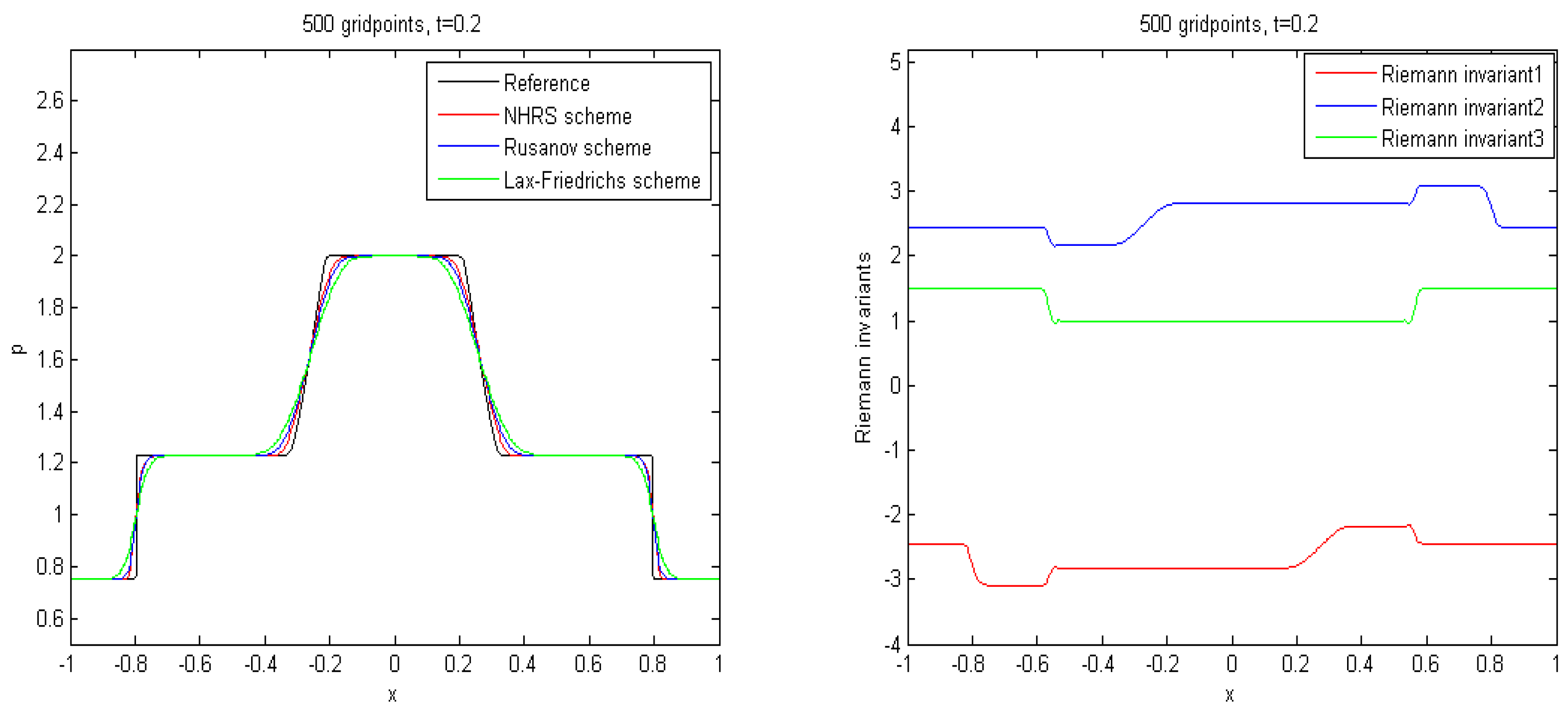
The solution includes two shock, two contact discontinuity, and two rarefaction waves. The domain [−1, 1] is divided into 500 mesh points, and the numerical simulation is implemented at time $t=0.2\mathrm{s}$. Figure 9 and Figure 10 show the numerical simulation for the water height, discharge, pressure, and temperature utilizing the NHRS scheme compared with the Lax–Friedrichs, the Rusanov scheme, and the reference solution at 5000 grid points. Figure 10 depicts the variation of Riemann invariants during computational time.

4.4. Example 4

The initial conditions corresponding to the following homogeneous case are

$$(h,u,\theta )=\left\{\begin{array}{c}(2,0.5,1)\mathrm{if}x\le 0,\hfill \\ (1,0.75,1.55)\mathrm{if}x>0.\hfill \end{array}\right.$$

(31)

The solution includes a fan, a contact discontinuity, and a shock wave. The domain [−1, 1] is divided into 300 mesh points, and the numerical simulation is computed at time $t=0.3\mathrm{s}$. Figure 11 and Figure 12 show the numerical results for the water height, variation of parameter of control, temperature, pressure, and Riemann invariants using the NHRS scheme.

Second, we will simulate our scheme for the Ripa model with non flat bottom topography:

4.5. Example 5: Perturbation of a Lake at Rest Problem

We consider a small perturbation of a lake at rest problem with the following initial conditions

$$Z(x,0)=\left\{\begin{array}{c}0.85\left\{Cos\left[10\pi \right(x+0.9\left)\right]+1\right\}\mathrm{if}-1\le x\le -0.8,\hfill \\ 1.25\left\{Cos\left[10\pi \right(x-0.4\left)\right]+1\right\}\mathrm{if}0.3\le x\le 0.5,\hfill \\ 0\mathrm{Otherwise},\hfill \end{array}\right.$$

(32)

$$h+Z=6,u=0\mathrm{and}\theta =4.$$

We run the NHRS scheme utilizing 200 mesh points and time $t=1\mathrm{s}$. We note that the proposed scheme conserves the steady state solution. The computational domain [−1, 1] is divided into 200 grid points. Figure 13 and Figure 14 show the numerical simulation for the free surface, discharge, $h\theta$, and pressure. We note that the NHRS scheme conserves the steady state solution.

4.6. Example 6

We consider the Ripa model with the discontinuous topography with the following initial conditions:

$$(h,u,\theta ,Z)=\left\{\begin{array}{c}(20,3,10,0)\mathrm{if}x\le 300,\hfill \\ (25,10,5,3)\mathrm{if}x>300.\hfill \end{array}\right.$$

(33)

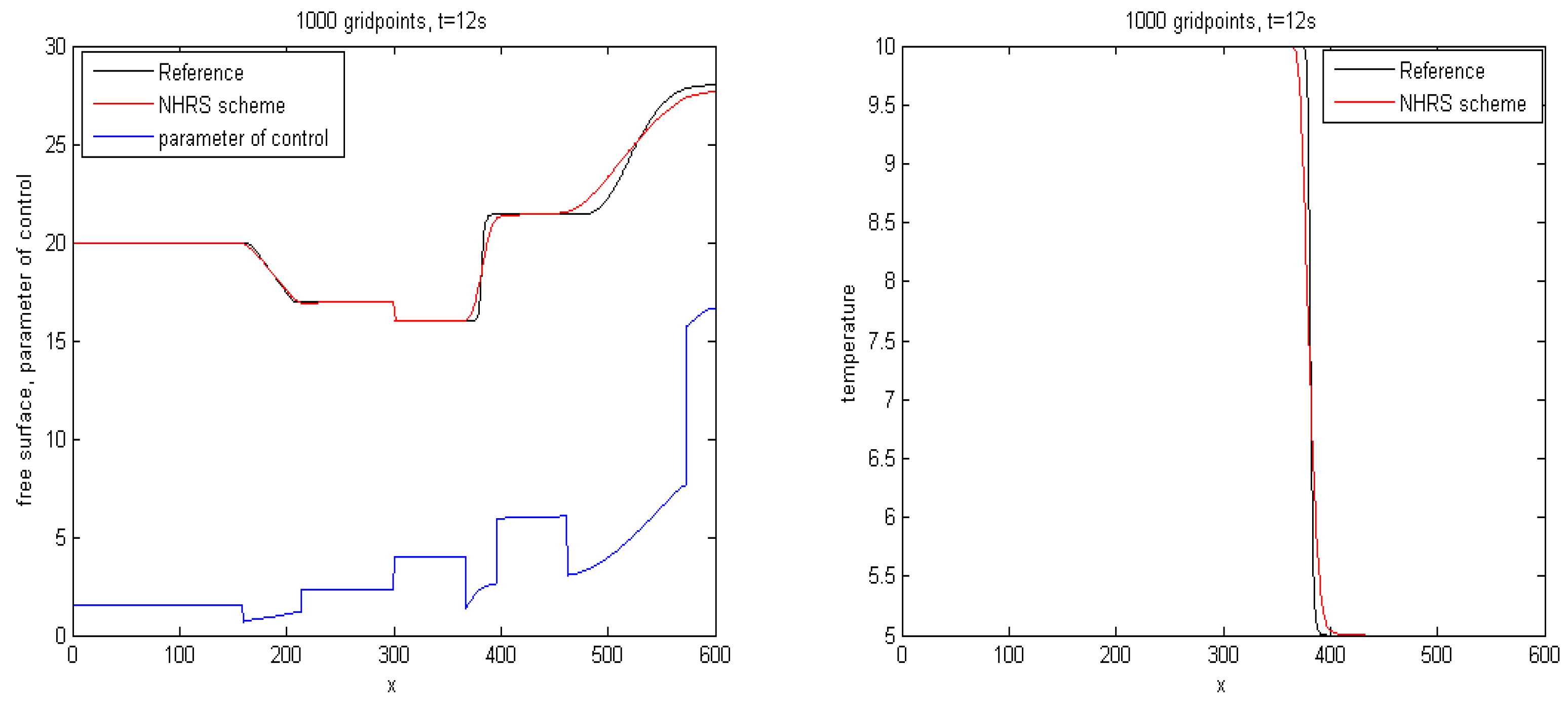
The domain is [0, 600] with 500 mesh points and time $t=12\mathrm{s}$. The solution includes a fan, a stationary shock, and a contact discontinuity and fan. Figure 15 and Figure 16 display the numerical results for the free surface and variation of ${\alpha }_{i+\frac{1}{2}}^n$, temperature, pressure, and variation of Riemann invariants during computational time. These results compare with reference solution acquired from the NHRS scheme with 10,000 grid points.

4.7. Example 7

We take into account the Ripa model via discontinuous topography for the initial conditions:

$$(h,u,\theta ,Z)=\left\{\begin{array}{c}(10,-9,2,0)\mathrm{if}x\le 300,\hfill \\ (12,-5,1,3)\mathrm{if}x>300.\hfill \end{array}\right.$$

(34)

The computational domain and time are [0, 600] and $t=12\mathrm{s}$, respectively. We implement the NHRS scheme using 1000 grid points. The solution includes a fan, contact discontinuity, and a fan and stationary shock. Figure 17 and Figure 18 display the numerical results for the water height, ${\alpha }_{i+\frac{1}{2}}^n$, temperature, pressure, and Riemann invariants obtained by using the NHRS scheme compared with the reference solution acquired from the NHRS scheme with 10,000 grid points.

4.8. Example 8

We take into account the Ripa model via discontinuous topography for the initial conditions:

$$(h,u,\theta ,Z)=\left\{\begin{array}{c}(20,0,10,0)\mathrm{if}x\le 300,\hfill \\ (15,0,5,3)\mathrm{if}x>300.\hfill \end{array}\right.$$

(35)

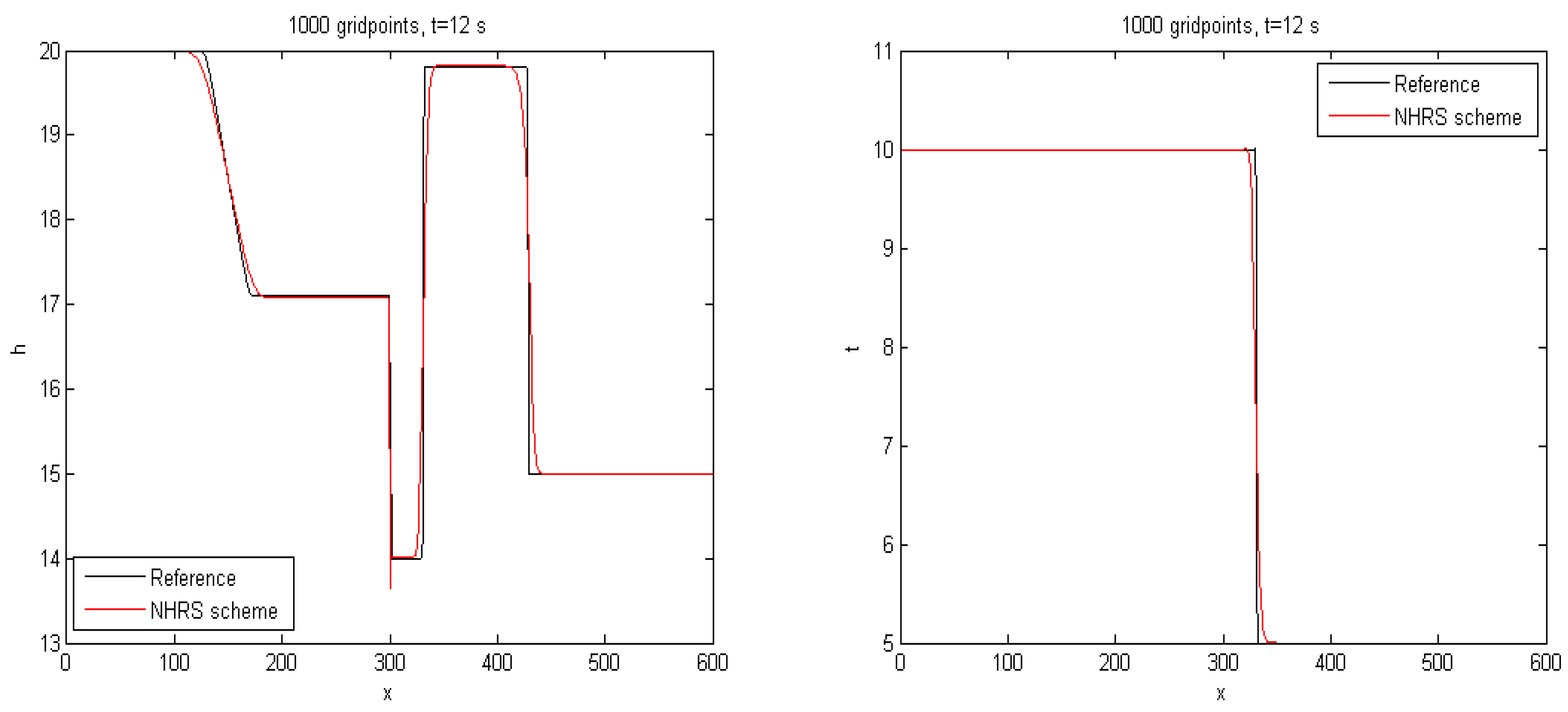
The domain and time are [0, 600] and $t=12\mathrm{s}$, respectively. We implement the NHRS scheme using 1000 mesh points. The solution includes a fan, a stationary shock, contact discontinuity, and stationary shock. Figure 19 and Figure 20 exhibit the numerical simulation for the water height, temperature, pressure, and ${\alpha }_{i+\frac{1}{2}}^n$. It is obtained by using the NHRS scheme compared with the reference solution for 10,000 grid points.

4.9. Example 9

We take into account the Ripa model via topography, and the following initial conditions can be written as:

$$Z\left(x\right)=\left\{\begin{array}{c}8\mathrm{if}|x-300|<75\hfill \\ 0\mathrm{Otherwise},\hfill \end{array}\right.$$

(36)

$$(h,u,\theta )=\left\{\begin{array}{c}(20-Z(x),0,10)\mathrm{if}x\le 300,\hfill \\ (15-Z(x),0,5)\mathrm{otherwise}.\hfill \end{array}\right.$$

(37)

The domain and time are [0, 600] and $t=12\mathrm{s}$, respectively. We implement the NHRS scheme using 1000 grid points. Figure 21 and Figure 22 display the numerical results for the free surface, ${\alpha }_{i+\frac{1}{2}}^n$, $h\theta$, pressure, and Riemann invariants, with 1000 grid points.

5. Conclusions

In this work, we considered the Ripa system without bottom topography and with topography. We implemented the NHRS scheme to solve the Ripa model. We compared the NHRS scheme with Lax–Friedrichs, the Rusanov scheme and the reference solution. Extensive numerical results show that the NHRS scheme gives high order accuracy and admits perfect resolutions for smooth and discontinuous solutions. In superfluid energy applications and many other fields, the solutions offered are crucial. Our results show that the NHRS scheme is an efficient tool for solving such balance laws.

In a forthcoming paper, we will consider the 2D Ripa system, which is given by [19]:

$$\begin{array}{c}{\left(h\right)}_t+{\left(hu\right)}_x+{\left(hv\right)}_y=0,\hfill \\ {\left(hu\right)}_t+{(h{u}^2+\frac{g{h}^2\theta }{2})}_x+{\left(huv\right)}_y=-gh\theta Z_x,\hfill \\ {\left(hv\right)}_t+{\left(huv\right)}_x+{(h{v}^2+\frac{g{h}^2\theta }{2})}_y=-gh\theta Z_y,\hfill \\ {\left(h\theta \right)}_t+{\left(hu\theta \right)}_x+{\left(hv\theta \right)}_y=0.\hfill \end{array}$$

(38)

However, it may be very difficult to rebuilt a traditional scheme for the Ripa model (38) because its eigensystem may be incomplete because of the resonance phenomenon. Thus, computing the Riemann problem solution becomes extremely challenging. As a result, we would like to employ the NHRS technique, which avoids the resolution of the Riemann issues.

References

1. Shakeel, M.; Mohyud-Din, S.T.; Iqbal, M.A. Modified extended exp-function method for a system of nonlinear partial differential equations defined by seismic sea waves. Pramana 2018, 91, 28. [Google Scholar] [CrossRef]
2. Chunga, K.; Toulkeridis, T. Ftrst evidence of plaeo-tsunami deposits of a major historic event in Ecuador. J. Tsunami Soc. Int. 2014, 33, 55–69. [Google Scholar]
3. Pedlosky, J. Geophysical Fluid Dynamics, 2nd ed.; Springer: New York, NY, USA, 1987. [Google Scholar]
4. Salmon, R. Lectures on Geophysical Fluid Dynamics; Oxford University Press: Oxford, UK, 1998. [Google Scholar]
5. Abdelrahman, M.A.E. On the shallow water equations. Z. Naturforsch. 2017, 72, 873–879. [Google Scholar] [CrossRef]
6. Ripa, P. Conservation laws for primitive equations models with inhomogeneous layers. Geophys. Astrophys. Fluid Dynam. 1993, 70, 85–111. [Google Scholar] [CrossRef]
7. Dellar, P.J. Common Hamiltonian structure of the shallow water equations with horizontal temperature gradients and magnetic fields. Phys. Fluids 2003, 15, 292–297. [Google Scholar] [CrossRef]
8. Ripa, P. On improving a one-Layer ocean model with thermodynamics. J. Fluid Mech. 1995, 303, 169–201. [Google Scholar] [CrossRef]
9. Keimer, A.; Pflug, L. Nonlocal conservation laws with time delay. Nonlinear Differ. Equ. Appl. 2019, 26, 54. [Google Scholar] [CrossRef]
10. Rodriguez, D.F.N.; Wintrant, E.; Sename, O. Control-oriented modeling of fluid networks: A time-delay approach. In Recent Results on Nonlinear Delay Control Systems; Springer International Publishing: Cham, Switzerland, 2016. [Google Scholar]
11. Greenberg, J.M.; Leroux, A.Y. A Well-balanced scheme for the numerical processing of source terms in hyperbolic equations. SIAM J. Numer. Anal. 1996, 33, 1–16. [Google Scholar] [CrossRef]
12. Krner, D.; Thanh, M.D. Numerical solutions to compressible flows in a nozzle with variable cross-section. SIAM J. Numer. Anal. 2005, 43, 796–824. [Google Scholar] [CrossRef]
13. Wen, X. A steady state capturing and preserving method for computing hyperbolic systems with geometrical source terms having concentrations. J.Comput. Phys. 2006, 219, 322–390. [Google Scholar] [CrossRef]
14. Desveaux, V.; Zenk, M.; Berthon, C.; Klingenberg, C. Well-Balanced schemes to capture non-Explicit steady states: Ripa model. Math. Comput. 2016, 85, 1571–1602. [Google Scholar] [CrossRef]
15. Britton, J.; Xing, Y. High order still-water and moving-water equilibria preserving discontinuous Galerkin methods for the Ripa model. J. Sci. Comput. 2020, 82, 30. [Google Scholar] [CrossRef]
16. Rehman, A.; Ali, I.; Zia, S.; Qamar, S. Well-balanced finite volume multi-resolution schemes for solving the Ripa models. Adv. Mech. Eng. 2021, 13, 1–16. [Google Scholar] [CrossRef]
17. Chertock, A.; Karni, S.; Kurganov, A. Interface tracking method for compressible multifluids. ESAIM Math. Model. Numer. Anal. 2008, 42, 991–1019. [Google Scholar] [CrossRef]
18. Chertock, A.; Kurganov, A.; Liu, Y. Central-upwind schemes for the system of shallow water equations with horizontal temperature gradients. Numer. Math. 2014, 127, 595–639. [Google Scholar] [CrossRef]
19. Touma, R.; Klingenberg, C. Well-balanced central finite volume methods for the Ripa system. Appl. Numer. Math. 2015, 97, 42–68. [Google Scholar] [CrossRef]
20. Audusse, E.; Bouchut, F.; Bristeau, M.-O.; Klein, R.; Perthame, B. A fast and stable well-balanced scheme with hydrostatic reconstruction for shallow water flows. SIAM J. Sci. Comput. 2004, 25, 2050–2065. [Google Scholar] [CrossRef] [Green Version]
21. Kurganov, A.; Levy, D. Central-upwind schemes for the Saint-Venant system. ESAIM Math. Model. Numer. Anal. 2002, 36, 397–425. [Google Scholar] [CrossRef] [Green Version]
22. Ricchiuto, M.; Bollermann, A. Stabilized residual distribution for shallow water simulations. J. Comput. Phys. 2009, 228, 1071–1115. [Google Scholar] [CrossRef]
23. Kurganov, A. Finite-volume schemes for shallow-water equations. Acta Numer. 2018, 27, 289–351. [Google Scholar] [CrossRef] [Green Version]
24. Xing, Y.; Shu, C.-W. A survey of high order schemes for the shallow water equations. J. Math. Study 2014, 47, 221–249. [Google Scholar]
25. Xing, Y.; Shu, C.-W.; Noelle, S. On the advantage of well-balanced schemes for moving-water equilibria of the shallow water equations. J. Sci. Comput. 2011, 48, 339–349. [Google Scholar] [CrossRef]
26. Han, X.; Li, G. Well-Balanced finite difference WENO schemes for the Ripa model. Comput. Fluids 2016, 134–135, 1–10. [Google Scholar] [CrossRef]
27. Snchez-Linares, C.; Luna, T.M.D.; Daz, M.J.C. A HLLC scheme for Ripa model. Appl. Math. Comput. 2016, 272, 369–384. [Google Scholar] [CrossRef]
28. Mohamed, K. Simulation Numérique en Volume Finis, de Problémes D’écoulements Multidimensionnels Raides, par un Schéma de Flux á Deux pas. Ph.D. Dissertation, University of Paris, Paris, France, 2005. [Google Scholar]
29. Mohamed, K.; Seaid, M.; Zahri, M. A finite volume method for scalar conservation laws with stochastic time-space dependent flux function. J. Comput. Appl. Math. 2013, 237, 614–632. [Google Scholar] [CrossRef] [Green Version]
30. Mohamed, K.; Sahmim, S.; Abdelrahman, M.A.E. A Predictor–corrector scheme for simulation of two-phase granular flows over a moved bed with a variable topography. Eur. J. Mech.-B/Fluids 2022, 96, 39–50. [Google Scholar] [CrossRef]
31. Mohamed, K.; Benkhaldoun, F. A modified Rusanov scheme for shallow water equations with topography and two phase flows. Eur. Phys. J. Plus 2016, 131, 207. [Google Scholar] [CrossRef]
32. Mohamed, K. A finite volume method for numerical simulation of shallow water models with porosity. Comput. Fluids 2014, 104, 9–19. [Google Scholar] [CrossRef]
33. Mohamed, K.; Alkhidhr, H.A.; Abdelrahman, M.A.E. The NHRS scheme for the Chaplygin gas model in one and two dimensions. AIMS Math. 2022, 7, 17785–17801. [Google Scholar] [CrossRef]
34. Mohamed, K.; Abdelrahman, M.A.E. The modified Rusanov scheme for solving the ultra-relativistic Euler equations. Eur. J. Mech. B/Fluids 2021, 90, 89–98. [Google Scholar] [CrossRef]
35. Rehman, A.; Ali, I.; Qamar, S. Exact riemann solutions of the ripa model for flat and non-flat bottom topographies. Res. Phys. 2018, 8, 104–113. [Google Scholar] [CrossRef]
Figure 1. Regions of four solutions corresponding to the Ripa model (10).
Fractalfract 06 00745 g001
Figure 2. Regions of five solutions corresponding to the Ripa model (16).
Fractalfract 06 00745 g002
Figure 3. Water height and temperature at t = 12 s.
Fractalfract 06 00745 g003
Figure 4. Pressure and discharge at t = 12 s.
Fractalfract 06 00745 g004
Figure 5. Parameter of control α i + 1 2 n and Riemann invariants at t = 0.5 s.
Fractalfract 06 00745 g005
Figure 6. Water height and temperature at t = 0.04 s.
Fractalfract 06 00745 g006
Figure 7. Pressure and discharge at t = 0.04 s.
Fractalfract 06 00745 g007
Figure 8. Parameter of control α i + 1 2 n and Riemann invariants at t = 0.04 s.
Fractalfract 06 00745 g008
Figure 9. Water height and discharge at t = 0.2 s.
Fractalfract 06 00745 g009
Figure 10. Pressure and Riemann invariants at t = 0.2 s.
Fractalfract 06 00745 g010
Figure 11. Water height and temperature at t = 0.3 s.
Fractalfract 06 00745 g011
Figure 12. Pressure and Riemann invariants at t = 0.3 s.
Fractalfract 06 00745 g012
Figure 13. Free surface and discharge at t = 1 s.
Fractalfract 06 00745 g013
Figure 14. h θ and pressure at t = 1 s.
Fractalfract 06 00745 g014
Figure 15. Free surface and α i + 1 2 n and temperature at t = 12 s.
Fractalfract 06 00745 g015
Figure 16. Pressure and Riemann invariants at t = 12 s.
Fractalfract 06 00745 g016
Figure 17. Water height and α i + 1 2 n and temperature at t = 12 s.
Fractalfract 06 00745 g017
Figure 18. Pressure and Riemann invariants at t = 12 s.
Fractalfract 06 00745 g018
Figure 19. Water height and temperature at t = 12 s.
Fractalfract 06 00745 g019
Figure 20. Pressure and Riemann invariants at t = 12 s.
Fractalfract 06 00745 g020
Figure 21. Free surface and α i + 1 2 n and h θ at t = 12 s.
Fractalfract 06 00745 g021
Figure 22. Pressure and Riemann invariants at t = 12 s.
Fractalfract 06 00745 g022
Publisher’s Note: MDPI stays neutral with regard to jurisdictional claims in published maps and institutional affiliations.