Article

Exact Fractional Solution by Nucci’s Reduction Approach and New Analytical Propagating Optical Soliton Structures in Fiber-Optics

by
Waqas Ali Faridi
1,
Muhammad Imran Asjad
1,* and
Sayed M. Eldin
2
1
Department of Mathematics, University of Management and Technology, Lahore 54782, Pakistan
2
Center of Research, Faculty of Engineering, Future University in Egypt, New Cairo 11835, Egypt
*
Author to whom correspondence should be addressed.
Fractal Fract. 2022, 6(11), 654; https://doi.org/10.3390/fractalfract6110654
Submission received: 13 October 2022 / Revised: 27 October 2022 / Accepted: 31 October 2022 / Published: 5 November 2022
(This article belongs to the Special Issue Recent Advances in Computational Physics with Fractional Application)

Abstract

:
This study examines the Chen–Lee–Liu dynamical equation, which represents the propagation of optical pulses in optical fibers and plasma. A new extended direct algebraic technique and Nucci’s scheme are used to find new solitary wave profiles. The method covers thirty-seven solitonic wave profiles, including approximately all soliton families, in an efficient and generic manner. New solitonic wave patterns are obtained, including a plane solution, mixed hyperbolic solution, periodic and mixed periodic solutions, mixed trigonometric solution, trigonometric solution, shock solution, mixed shock singular solution, mixed singular solution, complex solitary shock solution, singular solution and shock wave solutions. The exact fractional solution is obtained using Nucci’s reduction approach. The impact of the fractional order parameter on the solution is considered using both mathematical expressions and graphical visualization. The fractional order parameter is responsible for controlling the singularity of the solution which is graphically displayed. A sensitivity analysis was used to predict the sensitivity of equations with respect to initial conditions. To demonstrate the pulse propagation characteristics, while taking suitable values for the parameters involved, 2-D, 3-D, and contour graphics of the outcomes achieved are presented. The influence of the fractional order ζ is shown graphically. A periodic-singular wave with lower amplitude and dark-singular behaviour is inferred from the graphical behaviour of the trigonometric function solution H 1 and the rational function solution H 34 from the obtained solutions, respectively.

1. Introduction

Non-linear partial differential equations are a key means of thoroughly examining trends in non-linear physical processes. In the areas of plasma, fiber-optics, mathematical physics, telecommunication engineering, and optics, the Schrödinger equation is an excellent tool for more precisely interpreting complex physical non-linear models. The extraction of analytical exact solutions to the Schrödinger equations is an intriguing research area since exact solutions are fundamental for addressing the physical properties of non-linear systems in applied mathematics [1,2,3]. Du et al. [4] presented a simulation of non-local wave propagation in unbounded multi-scale mediums. Xie and Zhang [5] developed an efficient dissipation-preserving fourth-order difference solver for fractional-in-space non-linear wave equations. Tian and Engquist [6] studied non-local operators for modeling processes that have traditionally been described by local differential operators.
A number of methodologies and strategies have been developed to provide analytically exact solutions for partial differential equations with non-linearity, such as the Kudryashov method [7,8], the sine-Gordon expansion scheme [9,10], the bilinear neural network technique [11,12], the extended simple equation method [13], the F-expansion method [14,15], the unified auxiliary equation method [16,17], the G G expansion approach [18], the Hirota bilinear method [19], the generalized exponential function method [20], and many others [21,22,23,24,25,26].
Chirp-free brilliant optical solitons and chirped optical solitons were investigated by Biswas et al. In 2018, the authors of [27,28] used a semi-inverse procedure and extended the trial equation method for the Chen–Lee–Liu model. In 2019, A generic travelling wave solution was discovered by Kudryashov [29] using the Weierstrass function approach after analysing the Chen–Lee–Liu equation with perturbation effects. In 2020, Yldirim [30] investigated solitary wave patterns and applied the Riccati equation approach to the Chen–Lee–Liu model. In 2021, the Sardar sub-equation method was used by Esen et al. [31] to produce new analytical solutions for the Chen–Lee–Liu system.
Recently, Tarla et al. [32] identified twelve solutions for the perturbed Chen–Lee–Liu model using the Jacobi elliptic function approach, including trigonometric, exponential, hyperbolic trigonometric, dark-bright, singular, and periodic soliton solutions. There remain gaps in the literature and uncertainty surrounding many soliton-type solutions. To address this gap, a generalised new extended direct algebraic technique is proposed here. It yields 37 analytical solutions, almost all of which are soliton solutions, including trigonometric, mixed-shock singular, hyperbolic trigonometric, mixed singular, exponential, periodic, dark-bright, rational, complex solitary shock, singular, logarithmic, bright, dark, dark singular, shock wave, bright singular, and periodic singular solutions.
We utilize the Chen–Lee–Liu model with perturbation [32],
i H t + α H x x + i β | H | 2 H x = i γ H x + μ ( | H | 2 n H ) x + δ ( | H | 2 n ) x H ,
where μ and δ stand for self-steeping for short pulses and the non-linear dispersion coefficient, respectively, and γ represents the inter-model dispersion coefficient. The group velocity dispersion and the the non-linearity coefficient are α and β . The density of the complex wave function is specified by the variable n in the last Equation (1). The CLL model considered has applications in optical couplers, optoelectronic devices, soliton cooling and meta-materials and specifies the dynamics of solitary waves in optical fibers [32]. The truncated M-fractional Equation (1) becomes,
i 0 A D t ζ ( H ) + α 0 A D x x 2 ζ ( H ) + i β | H | 2 0 A D x ζ ( H ) = i γ 0 A D x ζ ( H ) + μ 0 A D x ζ ( | H | 2 H ) x + δ 0 A D x ζ ( | H | 2 ) H .
at n = 1 .
A new extended direct algebraic method applied to the perturbed (CLL) equation enables generation of a variety of solitons.
The paper is structured as follows: Section 1 provides an introduction. Section 2 describes the scheme and applications. Section 3 is devoted to providing graphical representations. Section 4 provides closing remarks.

2. Construction of Analytical Solutions

2.1. New Extended Direct Algebraic Method

Let us consider a non-linear PDE:
P ( H , H t , H x , H t t , H x x , ) = 0 ,
where the P polynomial function comprises the partial derivatives of H ( x , t ) . This can be converted to an ordinary differential equation:
Q ( Υ , Υ , Υ , ) = 0 .
The transformation is given in [32,33]:
H ( x , t ) = Υ ( ) e ι θ ,
where, = k 1 x + k 2 t , θ = k 3 x + k 4 t . The prime is a derivative with respect to ℧ in Equation (4). Let Equation (4) have the solution:
Υ ( ) = j = 0 m a j ( R ( ) ) j ,
where,
R ( ) = ln [ ρ ] B + A R ( ) + C R 2 ( ) , ρ 0 , 1 ,
C , B and A are real constants and = A 2 4 B C . The general roots concerning the parameters B , A and C of Equation (7) are:
(Family 1): When A 2 4 B C < 0 , and C 0 ,
R 1 ( ) = A 2 C + 2 C tan ρ 2 ,
R 2 ( ) = A 2 C 2 C cot ρ 2 ,
R 3 ( ) = A 2 C + 2 C tan ρ ± m n sec ρ ,
R 4 ( ) = A 2 C + 2 C cot ρ ± m n csc ρ ,
R 5 ( ) = A 2 C + 4 C tan ρ 4 cot ρ 4 .
(Family 2): When A 2 4 B C > 0 , and C 0 ,
R 6 ( ) = A 2 C 2 C tanh ρ 2 ,
R 7 ( ) = A 2 C 2 C coth ρ 2 ,
R 8 ( ) = A 2 C + 2 C tanh ρ ± i m n s e c h ρ ,
R 9 ( ) = A 2 C + 2 C coth ρ ± m n c s c h ρ ,
R 10 ( ) = A 2 C 4 C t a n h ρ 4 + c o t h ρ 4 .
(Family 3): When B C > 0 and A = 0 ,
R 11 ( ) = B C t a n ρ B C ,
R 12 ( ) = B C c o t ρ B C ,
R 13 ( ) = B C tan ρ 2 B C ± m n s e c ρ 2 B C ,
R 14 ( ) = B C c o t ρ 2 B C ± m n csc ρ 2 B C ,
R 15 ( ) = 1 2 B C tan ρ B C 2 cot ρ B C 2 .
(Family 4): When B C < 0 and A = 0 ,
R 16 ( ) = B C tanh ρ B C ,
R 17 ( ) = B C coth ρ B C ,
R 18 ( ) = B C tanh ρ 2 B C ± i m n s e c h ρ 2 B C ,
R 19 ( ) = B C coth ρ 2 B C ± m n c s c h ρ 2 B C ,
R 20 ( ) = 1 2 B C tanh ρ B C 2 + c o t h ρ B C 2 .
(Family 5): When A = 0 and B = C ,
R 21 ( ) = tan ρ B ,
R 22 ( ) = cot ρ B ,
R 23 ( ) = tan ρ 2 B ± m n sec ρ 2 B ,
R 24 ( ) = cot ρ 2 B ± m n csc ρ 2 B ,
R 25 ( ) = 1 2 tan ρ B 2 cot ρ B 2 .
(Family 6): When A = 0 and C = B ,
R 26 ( ) = tanh ρ B ,
R 27 ( ) = coth ρ B ,
R 28 ( ) = tanh ρ 2 B ± i m n s e c h ρ 2 B ,
R 29 ( ) = cot ρ 2 B ± m n c s c h ρ 2 B ,
R 30 ( ) = 1 2 tanh ρ B 2 + cot ρ B 2 .
(Family 7): When A 2 = 4 B C ,
R 31 ( ) = 2 B ( A ln [ ρ ] + 2 ) A 2 ln [ ρ ] .
(Family 8): When B = p q , ( q 0 ) , A = p , and C = 0 ,
R 32 ( ) = ρ p q .
(Family 9): When A = C = 0 ,
R 33 ( ) = B ln [ ρ ] .
(Family 10): When A = B = 0 ,
R 34 ( ) = 1 C ln [ ρ ] .
(Family 11): When B = 0 and A 0 ,
R 35 ( ) = m A C cosh ρ A sinh ρ A + m ,
R 36 ( ) = A sinh ρ A + cosh ρ A C sinh ρ A + cosh ρ A + n .
(Family 12): When C = p q , ( q 0 ) , A = p , and B = 0 ,
R 37 ( ) = m ρ p m q n ρ p .
sinh ρ ( ) = m ρ n ρ 2 , cosh ρ ( ) = m ρ + n ρ 2 ,
tanh ρ ( ) = m ρ n ρ m ρ + n ρ , coth ρ ( ) = m ρ + n ρ m ρ n ρ ,
s e c h ρ ( ) = 2 m ρ + n ρ , c s c h ρ ( ) = 2 m ρ n ρ ,
s i n ρ ( ) = m ρ i n ρ i 2 i , c o s ρ ( ) = m ρ i + n ρ i 2 ,
tan ρ ( ) = i m ρ i n ρ i m ρ i + n ρ i , cot ρ ( ) = i m ρ i + n ρ i m ρ i n ρ i ,
sec ρ ( ) = 2 m ρ + n ρ , csc ρ ( ) = 2 i m ρ n ρ ,
where m , n > 0 are arbitrary constant deformation parameters.

2.2. Application to the Equation (3)
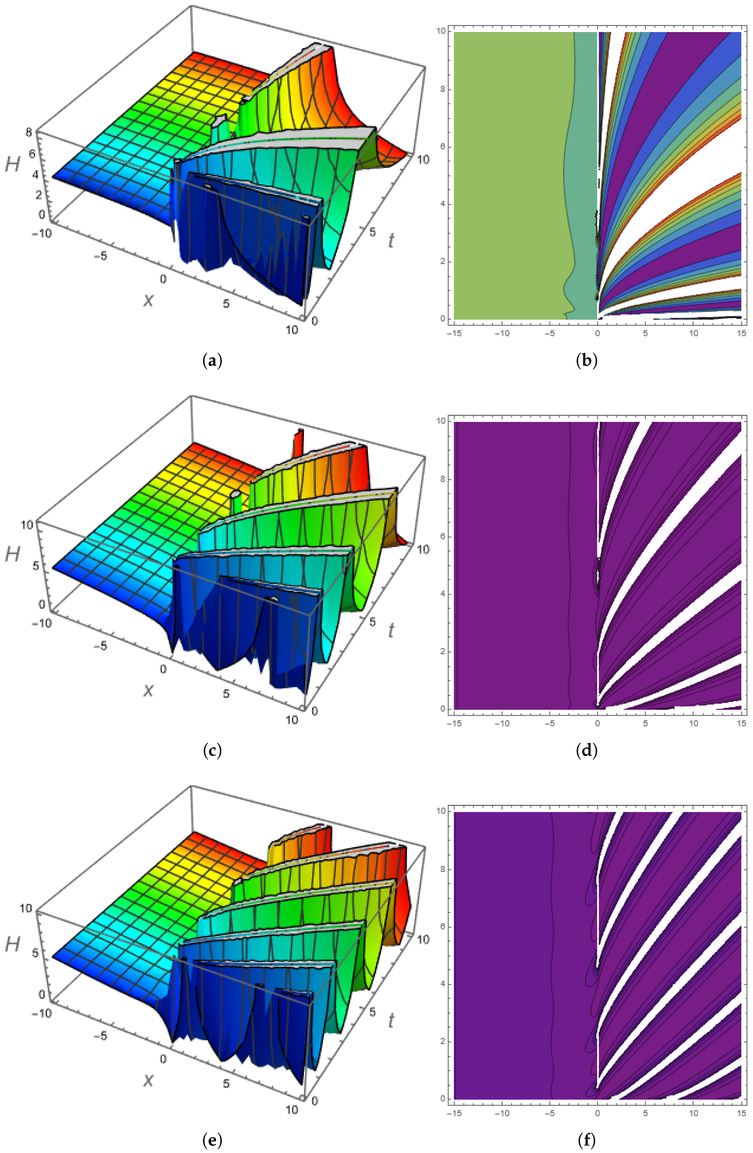
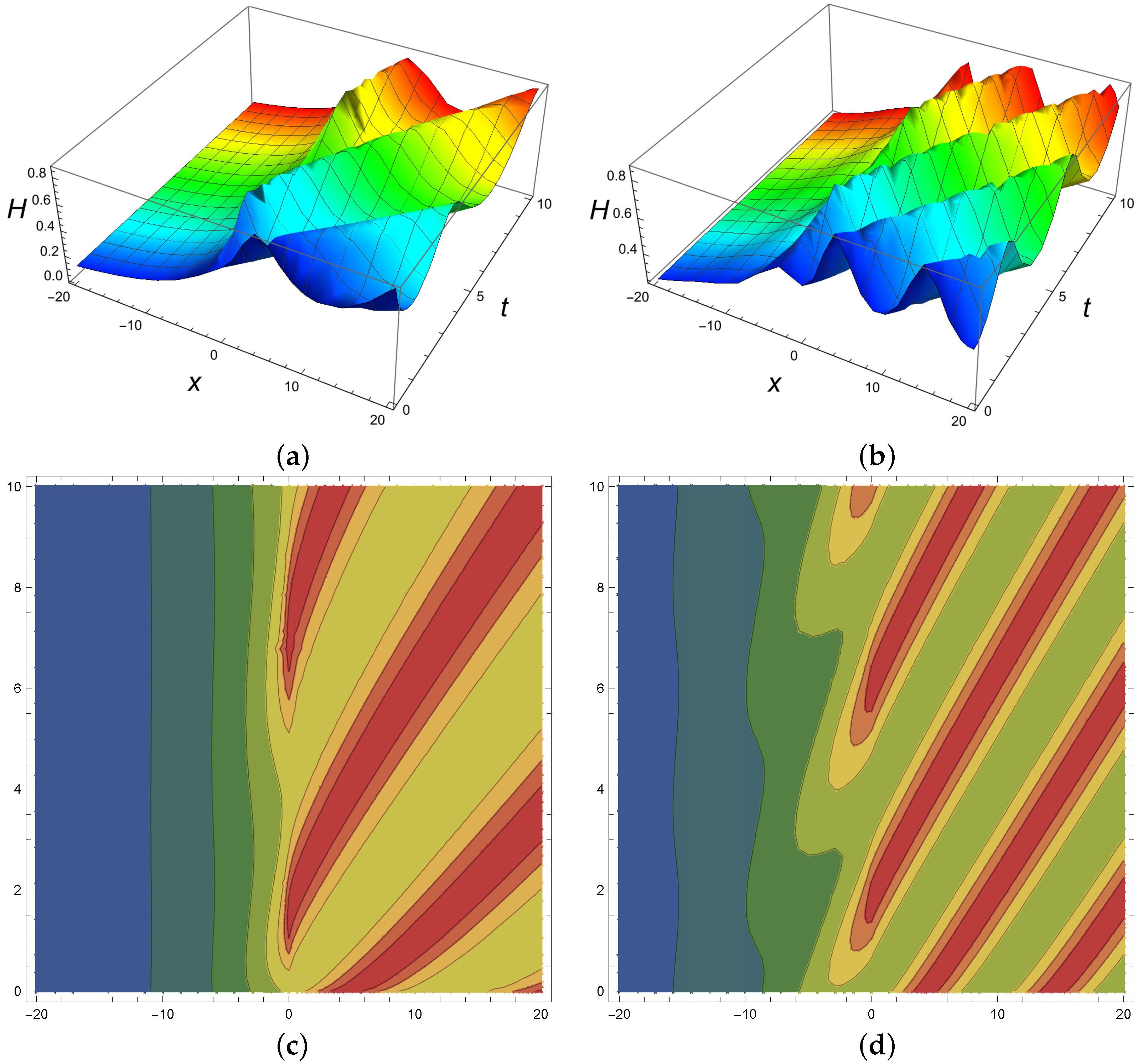
We use a fractional travelling wave transformation [32,33] to identify solutions to the Equation (2):
H ( x , t ) = Υ ( ) e i θ , where , = Γ [ σ + 1 ] ζ ( x ζ λ t ζ ) , θ ( x , t ) = Γ [ σ + 1 ] ζ ( κ x ζ + ω t ζ + η ) .
Equation (2) is subjected to the travelling wave transformation (45), resulting in an ordinary differential equation.
i λ Υ ω Υ + α Υ 2 i κ α Υ κ 2 α Υ + i β Υ Υ 2 + κ β Υ 3 i γ Υ κ γ Υ 3 i μ Υ Υ 2 κ μ Υ 3 2 i δ Υ Υ 2 = 0 .
Now, the given ordinary differential equation’s real and imaginary components may be derived.
κ ( β μ ) Υ 3 + α Υ ( ω + α κ 2 + γ κ ) Υ = 0 .
( β 3 μ 2 δ ) Υ Υ 2 ( λ + 2 α κ + γ ) Υ = 0 .
By setting the imaginary part components to zero, we get β = 3 μ + 2 δ and λ = ( γ + 2 α κ ) . The real component (47) becomes subject to the aforementioned two constraints,
2 κ ( δ + μ ) Υ 3 + α Υ ( ω + α κ 2 + γ κ ) Υ = 0 .
For Equation (49), the homogeneous balancing principle results in j = 1 . As a result, the solution (53) for the Equation (49) may be written as,
Υ ( ) = a 0 + a 1 R ( ) ,
where, R ( ) = ln [ ρ ] B + A R ( ) + C R 2 ( ) , ρ 0 , 1 . Equation (50) is placed into Equation (49) and the system of equations is obtained by collecting coefficients of different powers of R .
R 0 : α A B ln [ ρ ] 2 a 1 + 2 κ ( μ + δ ) a 0 3 ( α κ 2 + γ κ + ω ) a 0 = 0 , R 1 : α ( A 2 + 2 C ) ln [ ρ ] 2 a 1 + 6 κ ( μ + δ ) a 0 2 a 1 ( α κ 2 + γ κ + ω ) a 1 = 0 , R 2 : 3 α A C ln [ ρ ] 2 a 1 + 6 κ ( μ + δ ) a 0 a 1 2 = 0 , R 3 : 2 α C 2 ln [ ρ ] 2 a 1 + 2 κ ( μ + δ ) a 1 3 = 0 .
The solution of the aforementioned system (51) is obtained by utilizing the Mathematica,
[ a 0 = ± A 2 α κ ( μ + δ ) ln [ ρ ] , a 1 = ± C α κ ( μ + δ ) ln [ ρ ] , ω = κ ( γ + α κ ) α 2 ln [ ρ ] 2 ]
After substituting (52) into (50), we get,
H ( x , t ) = Λ A 2 + C R i ( x λ t ) e i ( κ x + ω t + η ) ,
where Λ = ± α κ ( μ + δ ) ln [ ρ ] .
It can be seen that we can obtain many solutions by taking R i ( ) from (8)–(44).
(Family 1): When A 2 4 B C < 0 and C 0 .
The mixed trigonometric solutions are obtained as,
H 1 ( x , t ) = Λ 2 tan ρ 2 e i θ ,
H 2 ( x , t ) = Λ 2 cot ρ 2 ) e i θ ,
H 3 ( x , t ) = Λ 2 tan ρ ± m n sec ρ e i θ ,
H 4 ( x , t ) = Λ 2 cot ρ ± m n csc ρ e i θ ,
H 5 ( x , t ) = Λ 4 tan ρ 4 cot ρ 4 ) e i θ .
(Family 2): When A 2 4 B C > 0 and C 0 .
The shock solution is obtained as,
H 6 ( x , t ) = Λ 2 tanh ρ 2 e i θ ,
The singular solution is obtained as,
H 7 ( x , t ) = Λ 2 coth ρ 2 e i θ ,
The mixed complex solitary-shock solution is obtained as,
H 8 ( x , t ) = Λ 2 tanh ρ ± i m n s e c h ρ ) e i θ ,
The mixed singular solution is obtained as,
H 9 ( x , t ) = Λ 2 coth ρ ± m n c s c h ρ ) e i θ ,
The mixed shock-singular solution is obtained as,
H 10 ( x , t ) = Λ 4 tanh ρ 4 + coth ρ 4 ) e i θ .
(Family 3): When B C > 0 and A = 0 .
The trigonometric solutions are obtained as,
H 11 ( x , t ) = Λ B C tan ρ B C e i θ ,
H 12 ( x , t ) = Λ B C cot ρ B C e i θ ,
The mixed trigonometric solutions are obtained as,
H 13 ( x , t ) = Λ B C tan ρ 2 B C ± m n sec ρ 2 B C e i θ ,
H 14 ( x , t ) = Λ B C cot ρ 2 B C ± m n csc ρ 2 B C e i θ ,
H 15 ( x , t ) = Λ 2 B C tan ρ B C 2 cot ρ B C 2 e i θ .
(Family 4): When B C < 0 and A = 0 .
The shock-wave solution is obtained as,
H 16 ( x , t ) = Λ B C tanh ρ B C e i θ ,
The singular solution is obtained as,
H 17 ( x , t ) = Λ B C coth ρ B C e i θ ,
The different complex combo-type solutions are obtained as,
H 18 ( x , t ) = Λ B C tanh ρ 2 B C ± i m n s e c h ρ 2 B C ) e i θ ,
H 19 ( x , t ) = Λ B C coth ρ 2 B C ± m n c s c h ρ 2 B C ) e i θ ,
H 20 ( x , t ) = Λ 2 B C tanh ρ B C 2 + coth ρ B C 2 ) e i θ .
(Family 5): When A = 0 and B = C .
The periodic and mixed-periodic wave solutions are obtained as,
H 21 ( x , t ) = B Λ tan ρ B e i θ ,
H 22 ( x , t ) = B Λ cot ρ B e i θ ,
H 23 ( x , t ) = B Λ tan ρ 2 B ± m n sec ρ 2 B e i θ ,
H 24 ( x , t ) = B Λ cot ρ 2 B ± m n csc ρ 2 B e i θ ,
H 25 ( x , t ) = B Λ 2 tan ρ B 2 cot ρ B 2 e i θ .
(Family 6): When A = 0 and C = B .
The single and mixed-periodic wave solutions are obtained in the following forms,
H 26 ( x , t ) = B Λ tanh ρ B e i θ ,
H 27 ( x , t ) = B Λ coth ρ B e i θ ,
H 28 ( x , t ) = B Λ tanh ρ 2 B ± i m n s e c h ρ 2 B e i θ ,
H 29 ( x , t ) = B Λ cot ρ 2 B ± m n c s c h ρ 2 B e i θ ,
H 30 ( x , t ) = B Λ 2 tanh ρ B 2 + cot ρ B 2 e i θ .
(Family 7): When A 2 = 4 B C .
We derive only one solution as,
H 31 ( x , t ) = Λ A 2 2 C B ( A ln ρ + 2 ) A 2 ln ρ e i θ .
(Family 8): When A = p , B = p q , ( q 0 ) and C = 0 .
H 32 ( x , t ) = Constant .
(Family 9): When A = C = 0 ,
H 33 ( x , t ) = 0 .
(Family 10): When A = B = 0 .
We derive only one solution as,
H 34 ( x , t ) = Λ ln ρ e i θ .
(Family 11): When B = 0 and A 0 .
The mixed hyperbolic solutions are obtained as,
H 35 ( x , t ) = Λ A 1 2 m Λ A cosh ρ A sinh ρ A + m e i θ ,
H 36 ( x , t ) = Λ A 1 2 sinh ρ A + cosh ρ A sinh ρ A + cosh ρ A + n e i θ .
(Family 12): When A = p , C = p q , ( q 0 and B = 0 ) .
The plane solution is obtained in the following form,
H 37 ( x , t ) = Λ A 2 C m ρ p m q n ρ p e i θ .

3. Graphical Study

This section is devoted to graphical visualization of the obtained solutions.
Figure 1a,b present periodic-singular, 3-D and contour profiles of the trigonometric function solution at fractional order 0.1 .
Figure 1c,d present periodic-singular, 3-D and contour profiles of the trigonometric function solution at fractional order 0.5 .
Figure 1e,f present periodic-singular, 3-D and contour profiles of the trigonometric function solution at fractional order 0.7 .
Remark 1. 
As the fractional order moves towards the classical order, the singularity decreases. The behaviour of the solution is not periodic with fractional order, while the solution is periodic with classical periodic at the negative axis.
Figure 2a,b present bright soliton 3-D and contour profiles of the rational function solution at fractional order 0.1 .
Figure 2c,d present bright soliton 3-D and contour profiles of the trigonometric function solution at fractional order 0.5 .
Figure 2e,f present almost bright solitons with less amplitude 3-D and contour profiles of the rational function solution at fractional order 0.7 .
Remark 2. 
Figure 1 presents the mixed-kink and periodic solution. As the fractional order moves towards the classical order, the periodicity of behaviour also increases and the amplitude of the soliton wave decreases. The bright soliton is going to be flat as the simple rational solution in Figure 2.
Figure 3a,b show the two-dimensional effects of fractional order and comparison to the classical order for solutions H 1 and H 34 , respectively.
Figure 4 and Figure 5 are presenting the graphical behaviour of the exact solution which is obtained by Nucci’s reduction method.

4. Nucci’s Reduction Approach

We use the reduction approach in this stage [34]. If we assume that the variables change according to Galilean transformation, when employing this approach
Υ ( ) = λ 1 ( ) , Υ ( ) = λ 2 ( ) .
The ordinary differential Equation (46) can be transformed into the planer dynamical system, such as,
d λ 1 d = λ 2 , d λ 2 d = ω + α κ 2 + γ κ α λ 1 2 κ ( δ + μ ) α λ 1 3 .
The aforementioned system (91) being autonomous, we may now choose λ 1 as a new independent variable. As a result, system (91) becomes,
d λ 2 d λ 1 = ω + α κ 2 + γ κ λ 2 α λ 1 2 κ ( δ + μ ) λ 2 α λ 1 3 .
This is a first-order separable ODE with the exact solution provided by one time integration,
λ 2 λ 1 = ± α κ 2 + γ κ + ω λ 1 2 α κ δ + μ λ 1 4 α + 2 φ 0 ,
where, φ 0 is the integration constant and yields the first integral such as,
φ 0 = ( Υ ( ) ) 2 2 α κ 2 + γ κ + ω ( Υ 2 ( ) ) 2 α κ δ + μ ( Υ 4 ( ) ) 2 α .
Substituting Equation (93) into the first equation of the planer dynamical system (91) we get,
d λ 1 d = λ 1 α κ 2 + γ κ + ω α κ δ + μ λ 1 2 α + 2 φ 0 .
The Equation (95) is also a first-order separable equation, and, hence, the general solution is,
H ( x , t ) = i α κ 2 + γ κ + ω 1 + tanh 2 α κ 2 + γ κ + ω α + φ 1 α κ 2 + γ κ + ω κ δ + μ e i θ ( x , t ) ,
whenever φ 0 = 0 .
H ( x , t ) = ± e i θ ( x , t ) α κ 2 + γ κ α 2 κ 4 + 2 α γ κ 3 + 8 α δ κ φ 0 + 2 α κ 2 ω + 8 α κ μ φ 0 + γ 2 κ 2 + 2 γ κ ω + ω 2 + ω α φ 0 2 JacobiSN ( Z , K ) ,
whenever φ 0 0 .
Z = 1 2 α ( 2 α ( α κ 2 + γ κ α 2 κ 4 + 2 α γ κ 3 + 8 α δ κ φ 0 + 2 α κ 2 ω + 8 α κ μ φ 0 + γ 2 κ 2 + 2 γ κ ω + ω 2 + ω ) ) 1 2 ,
K = 1 2 ( 1 α φ 0 κ δ + μ ( α 2 κ 4 + 2 α γ κ 3 + γ 2 κ 2 + α 2 κ 4 + 2 α γ κ 3 + 8 α δ κ φ 0 + 2 α κ 2 ω + 8 α κ μ φ 0 + γ 2 κ 2 + 2 γ κ ω + ω 2 α κ 2 + 4 α δ κ φ 0 + 2 α κ 2 ω + 4 α κ μ φ 0 + γ α 2 κ 4 + 2 α γ κ 3 + 8 α δ κ φ 0 + 2 α κ 2 ω + 8 α κ μ φ 0 + γ 2 κ 2 + 2 γ κ ω + ω 2 κ + 2 γ κ ω + α 2 κ 4 + 2 α γ κ 3 + 8 α δ κ φ 0 + 2 α κ 2 ω + 8 α κ μ φ 0 0 + γ 2 κ 2 + 2 γ κ ω + ω 2 ω + ω 2 ) ) 1 2 ,
where = Γ [ σ + 1 ] ζ ( x ζ λ t ζ ) , θ ( x , t ) = Γ [ σ + 1 ] ζ ( κ x ζ + ω t ζ + η ) .

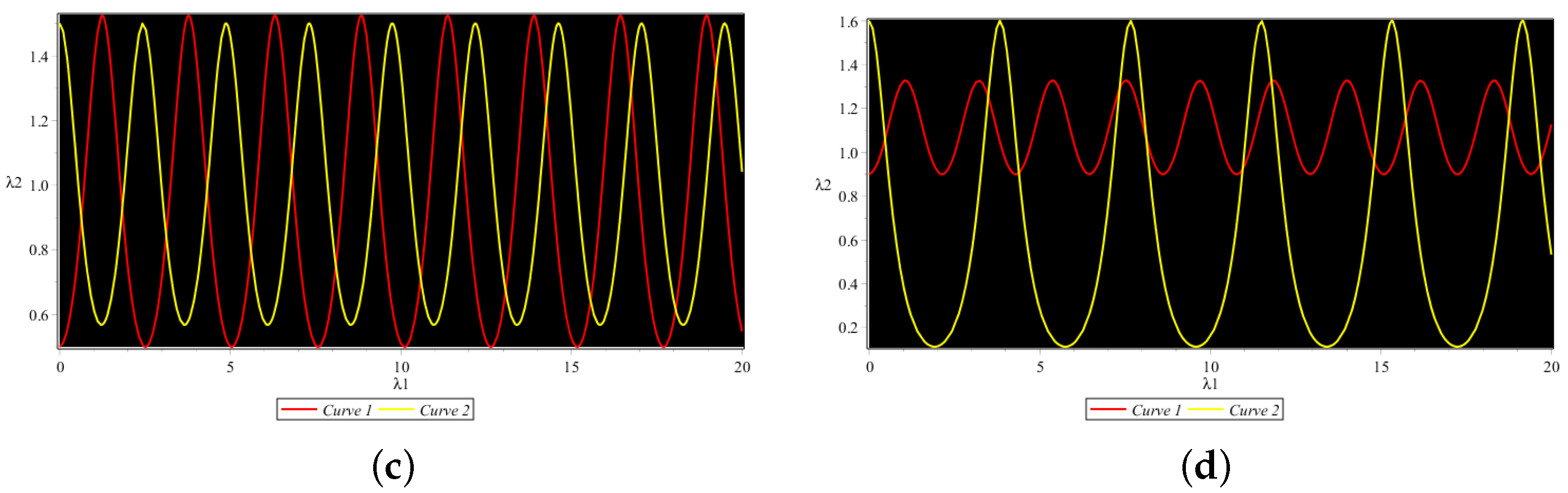
Sensitivity Assessment

This section describes the sensitive behaviour of the planer dynamical system (91) to check the sensitivity of the governing model. A sensitivity analysis is performed taking into account the parametric values ω = 1 , α = 1.5 , κ = 0.9 , μ = 2 , γ = 5 , δ = 0.9 .
From Figure 6 it can be seen that only minor changes in the initial values have a large impact on the dynamics of model. This means that the system is sensitive with respect to the initial value.

5. Conclusions

In this study, by utilising one of the generalised expansion strategies, several novel soliton solutions to the Chen–Lee–Liu model with perturbation term are achieved. The new extended direct algebraic approach provides 37 alternative varieties of soliton patterns.
  • The acquired types of soliton include exponential, plane wave solution, shock wave solution, rational, mixed-shock wave, trigonometric, complex shock wave solution, hyperbolic trigonometric, periodic, singular, singular shock wave solution, dark-singular, brilliant singular, and dark-bright solitons.
  • The solutions are presented in 2-D, 3-D and contour profiles.
  • A new fractional exact solution is obtained by utilizing Nucci’s reduction method.
  • The governing model is very sensitive with respect to the initial conditions.
  • For solution H 1 , the fractional-order shows more exciting behaviour, such as a larger singularity as ζ moves to the classical order and bright solution behaviour is produced when the fractional-order moves to the classical order for solution H 34 .
To demonstrate the graphical behaviour of optical pulses utilising the given analytical solutions, some suitable values were selected for the associated free parameters. The generated solutions can be used to interpret the non-linear model’s physical perspective. The new extended direct algebraic technique and Nucci’s reduction method represent strong and efficient mathematical techniques that may be used to provide exact analytical solutions to a variety of other challenging mathematical phenomena.

Author Contributions

Formal analysis, problem formulation: W.A.F.; Investigation, methodology: M.I.A. and W.A.F.; supervision, resources: M.I.A. and S.M.E.; validation, graphical discussion and software: M.I.A., W.A.F. and S.M.E.; funding: S.M.E.; review and editing. All authors have read and agreed to the published version of the manuscript.

Funding

This research received no external funding.

Informed Consent Statement

Not applicable.

Data Availability Statement

Data sharing not applicable to this article as no datasets were generated or analysed during the current study.

Acknowledgments

All the authors are obliged and thankful to the University of Management and Technology Lahore, Pakistan for facilitating and supporting the research.

Conflicts of Interest

The authors declare that they have no competing interests.

References

  1. Gao, W.; Ismael, H.F.; Bulut, H.; Baskonus, H.M. Instability modulation for the (2+1)-dimension paraxial wave equation and its new optical soliton solutions in Kerr media. Phys. Scr. 2020, 95, 035207. [Google Scholar] [CrossRef]
  2. Gao, W.; Ismael, H.F.; Husien, A.M.; Bulut, H.; Baskonus, H.M. Optical soliton solutions of the cubicquartic nonlinear Schrödinger and resonant nonlinear Schrödinger equation with the parabolic law. Appl. Sci. 2020, 10, 219. [Google Scholar] [CrossRef] [Green Version]
  3. Ali, K.K.; Yilmazer, R.; Yokus, A.; Bulut, H. Analytical solutions for the (3+1)-dimensional nonlinear extended quantum Zakharov-Kuznetsov equation in plasma physics. Phys. A Stat. Mech. Appl. 2020, 548, 124327. [Google Scholar] [CrossRef]
  4. Du, Q.; Zhang, J.; Zheng, C. Nonlocal wave propagation in unbounded multi-scale media. Commun. Comput. Phys. 2018, 24, 4. [Google Scholar] [CrossRef]
  5. Xie, J.; Zhang, Z. An effective dissipation-preserving fourth-order difference solver for fractional-in-space nonlinear wave equations. J. Sci. Comput. 2019, 79, 1753–1776. [Google Scholar] [CrossRef]
  6. Tian, X.; Engquist, B. Fast algorithm for computing nonlocal operators with finite interaction distance. arXiv 2019, arXiv:1905.08375. [Google Scholar] [CrossRef] [Green Version]
  7. Zafar, A.; Shakeel, M.; Ali, A.; Akinyemi, L.; Rezazadeh, H. Optical solitons of nonlinear complex Ginzburg-Landau equation via two modified expansion schemes. Opt. Quantum. Electron. 2022, 54, 5. [Google Scholar] [CrossRef]
  8. Srivastava, H.M.; Baleanu, D.; Machado, J.A.T.; Osman, M.S.; Rezazadeh, H.; Arshed, S.; Günerhan, H. Traveling wave solutions to nonlinear directional couplers by modified Kudryashov method. Phys. Scr. 2020, 95, 075217. [Google Scholar] [CrossRef]
  9. Fahim, M.R.A.; Kundu, P.R.; Islam, M.E.; Akbar, M.A.; Osman, M.S. Wave profile analysis of a couple of (3+1)-dimensional nonlinear evolution equations by sine-Gordon expansion approach. J. Ocean Eng. Sci. 2022, 7, 272–279. [Google Scholar] [CrossRef]
  10. Abdul Kayum, M.; Ali Akbar, M.; Osman, M.S. Stable soliton solutions to the shallow water waves and ion-acoustic waves in a plasma. Waves Random Complex Media 2020, 32, 1672–1693. [Google Scholar] [CrossRef]
  11. Zhang, R.; Bilige, S.; Chaolu, T. Fractal solitons, arbitrary function solutions, exact periodic wave and breathers for a nonlinear partial differential equation by using bilinear neural network method. J. Syst. Sci. Complex. 2021, 34, 122–139. [Google Scholar] [CrossRef]
  12. Zhang, R.F.; Bilige, S. Bilinear neural network method to obtain the exact analytical solutions of nonlinear partial differential equations and its application to p-gBKP equation. Nonlinear Dyn. 2019, 95, 3041–3048. [Google Scholar] [CrossRef]
  13. Khater, M.; Jhangeer, A.; Rezazadeh, H.; Akinyemi, L.; Akbar, M.A.; Inc, M.; Ahmad, H. New kinds of analytical solitary wave solutions for ionic currents on microtubules equation via two different techniques. Opt. Quantum Electron. 2021, 53, 609. [Google Scholar] [CrossRef]
  14. Karaman, B. The use of improved-F expansion method for the time-fractional Benjamin-Ono equation. Rev. Real Acad. Cienc. Exactas Físicas Nat. Ser. A Matemáticas 2021, 115, 128. [Google Scholar] [CrossRef]
  15. Yıldırım, Y. Optical solitons with Biswas-Arshed equation by F-expansion method. Optik 2021, 227, 165788. [Google Scholar] [CrossRef]
  16. Zayed, E.M.E.; Shohib, R.M.A. Solitons and Other Solutions for Two Higher-Order Nonlinear Wave Equations of KdV Type Using the Unified Auxiliary Equation Method. Acta Phys. Pol. A 2019, 136, 33–41. [Google Scholar] [CrossRef]
  17. Zayed, E.M.; Gepreel, K.A.; Shohib, R.M.; Alngar, M.E.; Yıldırım, Y. Optical solitons for the perturbed Biswas-Milovic equation with Kudryashov’s law of refractive index by the unified auxiliary equation method. Optik 2021, 230, 166286. [Google Scholar] [CrossRef]
  18. Ismael, H.F.; Bulut, H.; Baskonus, H.M. Optical soliton solutions to the Fokas-Lenells equation via sine-Gordon expansion method and ( m + G G )-expansion method. Pramana 2020, 94, 35. [Google Scholar] [CrossRef]
  19. Abdulkadir Sulaiman, T.; Yusuf, A. Dynamics of lump-periodic and breather waves solutions with variable coefficients in liquid with gas bubbles. Waves Random Complex Media 2021, 1–14. [Google Scholar] [CrossRef]
  20. Khodadad, F.S.; Mirhosseini-Alizamini, S.M.; Günay, B.; Akinyemi, L.; Rezazadeh, H.; Inc, M. Abundant optical solitons to the Sasa-Satsuma higher-order nonlinear Schröinger equation. Opt. Quantum Electron. 2021, 53, 702. [Google Scholar] [CrossRef]
  21. Ghanbari, B.; Kumar, S.; Niwas, M.; Baleanu, D. The Lie symmetry analysis and exact Jacobi elliptic solutions for the Kawahara-KdV type equations. Results Phys. 2021, 23, 104006. [Google Scholar] [CrossRef]
  22. Lü, D. Jacobi elliptic function solutions for two variant Boussinesq equations. Chaos Solitons Fractals 2005, 24, 1373–1385. [Google Scholar] [CrossRef]
  23. Baskonus, H.M.; Sulaiman, T.A.; Bulut, H. On the exact solitary wave solutions to the long-short wave interaction system. ITM Web Conf. 2018, 22, 01063. [Google Scholar] [CrossRef] [Green Version]
  24. Rehman, S.U.; Yusuf, A.; Bilal, M.; Younas, U.; Younis, M.; Sulaiman, T.A. Application of ( G G 2 )-expansion method to microstructured solids, magneto-electro-elastic circular rod and (2+1)-dimensional nonlinear electrical lines. Math. Eng. Sci. Aerosp. 2020, 11, 789–803. [Google Scholar]
  25. Zhang, R.F.; Li, M.C.; Yin, H.M. Rogue wave solutions and the bright and dark solitons of the (3+1)-dimensional Jimbo-Miwa equation. Nonlinear Dyn. 2021, 103, 1071–1079. [Google Scholar] [CrossRef]
  26. Zhang, Z.Y.; Liu, Z.H.; Miao, X.J.; Chen, Y.Z. Qualitative analysis and traveling wave solutions for the perturbed nonlinear Schrödinger’s equation with Kerr law nonlinearity. Phys. Letts. A 2011, 375, 1275–1280. [Google Scholar] [CrossRef]
  27. Biswas, A. Chirp-free bright optical soliton perturbation with Chen-Lee-Liu equation by traveling wave hypothesis and semi-inverse variational principle. Optik 2018, 172, 772–776. [Google Scholar] [CrossRef]
  28. Biswas, A.; Ekici, M.; Sonmezoglu, A.; Alshomrani, A.S.; Zhou, Q.; Moshokoa, S.P.; Belic, M. Chirped optical solitons of Chen-Lee-Liu equation by extended trial equation scheme. Optik 2018, 156, 999–1006. [Google Scholar] [CrossRef]
  29. Kudryashov, N.A. General solution of the traveling wave reduction for the perturbed Chen-Lee-Liu equation. Optik 2019, 186, 339–349. [Google Scholar] [CrossRef]
  30. Yıldırım, Y.; Biswas, A.; Asma, M.; Ekici, M.; Ntsime, B.P.; Zayed, E.M.; Moshokoa, S.P.; Alzahrani, A.K.; Belic, M.R. Optical soliton perturbation with Chen-Lee-Liu equation. Optik 2020, 220, 165177. [Google Scholar] [CrossRef]
  31. Esen, H.; Ozdemir, N.; Secer, A.; Bayram, M. On solitary wave solutions for the perturbed Chen-Lee-Liu equation via an analytical approach. Optik 2021, 245, 167641. [Google Scholar] [CrossRef]
  32. Tarla, S.; Karmina, K.A.; Yilmazer, R.; Osman, M.S. New optical solitons based on the perturbed Chen-Lee-Liu model through Jacobi elliptic function method. Opt. Quantum Electron. 2022, 54, 131. [Google Scholar] [CrossRef]
  33. Adil, J.; Faridi, W.A.; Asjad, M.I.; Inc, M. A comparative study about the propagation of water waves with fractional operators. J. Ocean Eng. Sci. 2022. [Google Scholar] [CrossRef]
  34. Xia, F.L.; Jarad, F.; Hashemi, M.S.; Riaz, M.B. A reduction technique to solve the generalized nonlinear dispersive mK (m, n) equation with new local derivative. Results Phys. 2022, 38, 105512. [Google Scholar] [CrossRef]
Figure 1. Trigonometric function solution of H 1 ( x , t ) for the values of α = 1 , κ = 0.1 , μ = 0.9 , δ = 0.01 , γ = 2 . (a) 3-D wave profile at fractional order ζ = 0.1 . (b) Contour wave profile at fractional order ζ = 0.1 . (c) 3-D wave profile at fractional order ζ = 0.5 . (d) Contour wave profile at fractional order ζ = 0.5 . (e) 3-D wave profile at fractional order ζ = 0.7 . (f) Contour wave profile at fractional order ζ = 0.7 .
Fractalfract 06 00654 g001
Figure 2. Rational function solution of H 34 ( x , t ) for the values of α = 1 , κ = 0.1 , μ = 0.9 , δ = 0.01 , γ = 2 . (a) 3-D wave profile at fractional order ζ = 0.1 . (b) Contour wave profile at fractional order ζ = 0.1 . (c) 3-D wave profile at fractional order ζ = 0.5 . (d) Contour wave profile at fractional order ζ = 0.5 . (e) 3-D wave profile at fractional order ζ = 0.7 . (f) Contour wave profile at fractional order ζ = 0.7 .
Fractalfract 06 00654 g002
Figure 3. Influence of fractional order with H 34 ( x , t ) for the values of α = 1 , κ = 0.1 , μ = 0.9 , δ = 0.01 , γ = 2 . (a) 2-D impact of fractional order ζ on solution H 1 . (b) 2-D impact of fractional order ζ on solution H 34 .
Fractalfract 06 00654 g003
Figure 4. New exact solution by Nucci’s method (96) for the values of α = 0.5 , κ = 0.2 , ω = 0.5 , δ = 0.01 , γ = 2 , φ 1 = 2.5 . (a) 3-D wave profile at fractional order ζ = 0.2 . (b) 3-D wave profile at fractional order ζ = 0.5 . (c) Contour wave profile at fractional order ζ = 0.2 . (d) Contour wave profile at fractional order ζ = 0.5 . (e) 2-D wave profile at fractional order ζ = 0.2 . (f) 2-D wave profile at fractional order ζ = 0.5 .
Fractalfract 06 00654 g004aFractalfract 06 00654 g004b
Figure 5. New exact solution by Nucci’s method (96) for the values of α = 0.5 , κ = 0.2 , ω = 0.5 , δ = 0.01 , γ = 2 , φ 1 = 2.5 . (a) 3-D wave profile at fractional order ζ = 0.7 . (b) 3-D wave profile at fractional order ζ = 0.9 . (c) Contour wave profile at fractional order ζ = 0.7 . (d) Contour wave profile at fractional order ζ = 0.9 . (e) 2-D wave profile at fractional order ζ = 0.7 . (f) 2-D wave profile at fractional order ζ = 0.9 .
Fractalfract 06 00654 g005aFractalfract 06 00654 g005b
Figure 6. Sensitivity analysis at different initial conditions. (a) Sensitive visualization for curve 1 at (1.5, 0.03) and curve 2 at (1.05, 0.02). (b) Sensitive visualization for curve 1 at (1, 0.03) and curve 2 at (1.04, 0.02). (c) Sensitive visualization for curve 1 at (0.5, 0.03) and curve 2 at (1.05, 0.02). (d) Sensitive visualization for curve 1 at (0.9, 0.03) and curve 2 at (1.6, 0.02).
Fractalfract 06 00654 g006aFractalfract 06 00654 g006b
Publisher’s Note: MDPI stays neutral with regard to jurisdictional claims in published maps and institutional affiliations.

