Article

A Novel Analytical LRPSM for Solving Nonlinear Systems of FPDEs

1
Department of Mathematical Sciences, Faculty of Science and Technology, Universiti Kebangsaan Malaysia (UKM), Bangi 43600, Malaysia
2
Department of Mathematics, Faculty of Arts and Science, Amman Arab University, Amman 11953, Jordan
*
Author to whom correspondence should be addressed.
Fractal Fract. 2022, 6(11), 650; https://doi.org/10.3390/fractalfract6110650
Submission received: 11 October 2022 / Revised: 28 October 2022 / Accepted: 31 October 2022 / Published: 4 November 2022

Abstract

:
This article employs the Laplace residual power series approach to study nonlinear systems of time-fractional partial differential equations with time-fractional Caputo derivative. The proposed technique is based on a new fractional expansion of the Maclurian series, which provides a rapid convergence series solution where the coefficients of the proposed fractional expansion are computed with the limit concept. The nonlinear systems studied in this work are the Broer-Kaup system, the Burgers’ system of two variables, and the Burgers’ system of three variables, which are used in modeling various nonlinear physical applications such as shock waves, processes of the wave, transportation of vorticity, dispersion in porous media, and hydrodynamic turbulence. The results obtained are reliable, efficient, and accurate with minimal computations. The proposed technique is analyzed by applying it to three attractive problems where the approximate analytical solutions are formulated in rapid convergent fractional Maclurian formulas. The results are studied numerically and graphically to show the performance and validity of the technique, as well as the fractional order impact on the behavior of the solutions. Moreover, numerical comparisons are made with other well-known methods, proving that the results obtained in the proposed technique are much better and the most accurate. Finally, the obtained outcomes and simulation data show that the present method provides a sound methodology and suitable tool for solving such nonlinear systems of time-fractional partial differential equations.

1. Introduction

Fractional-order systems have acquired a lot of attention and interest in various engineering and scientific fields as popular mathematical models used to describe real-world physical phenomena [1,2,3,4,5]. Fractional calculus provides a valuable instrument for showing the development of complicated dynamical systems with long-term memory impacts. In contrast to ordinary derivatives, defining fractional order derivatives of a specific function necessitates the existence of its complete history. Such a non-local feature, i.e., the memory consequence, has made it much more practical to explain various real-world physical systems using fractional differential equations. Investigating dynamics, including complexity, chaos, stability, bifurcation, and synchronization of these fractional order systems, has recently become an interesting research field in nonlinear sciences [6,7,8,9,10,11,12,13]. In order to study the real-world physical systems’ dynamic behavior, it is essential to determine how these solution trajectories can change over slight perturbations. Therefore, performing and developing various numerical techniques to analyze and simulate the systems’ nonlinear dynamics is important. Considering fractional derivatives, analytic-numeric approaches to fractional calculus frequently depend on versions of the Riemann-Liouville, Caputo, Grunwald-Letnikov, Riesz, or other approaches, which were discussed in previous studies during the past few years [14,15,16]. This study, however, will use Caputo’s approach of fractional differentiation, benefiting from Caputo’s approach that initial conditions of the fractional partial differential equations, i.e., (FPDEs) with Caputo’s derivatives take the same conventional form as in integer order.
Differential equations (DEs) can be used for modeling many chemical, biological, and physical phenomena. Because FPDEs have a significant impact on many applied disciplines, particularly nonlinear ones such as fluid flow, biological diffusion of populations, dynamical systems, control theory, electromagnetic waves, etc., there has been a growing interest in them in recent years [17,18,19,20,21]. Most scientific phenomena in various disciplines such as physics, biological systems, and engineering are nonlinear problems; therefore, it might be challenging to find their exact solutions, e.g., physical problems are typically modeled by utilizing higher nonlinear FPDEs, thereby finding exact solutions for these problems is quite challenging. Thus, numerical as well as approximate methods must be employed. Numerous useful techniques were used for solving linear and nonlinear FPDEs, including the variational iteration technique, the Adomian decomposition technique, the homotopy analysis technique, the homotopy perturbation technique, and the fractional residual power series technique [22,23,24,25,26,27,28].
The fractional power series method (FPSM) has been employed to solve several classes of differential and integral equations of the fractional order if the solution of the equation can be extended into a fractional power series [29]. Moreover, FPSM is a fast and easy method utilized to determine the fractional power series solution coefficients because if we compare the computational effort required to compute the solutions of the FPDEs in FPSM with other methods, it becomes clear that it is much less. Moreover, the results are much better, as the speed of implementation on mathematical packages helps to obtain the results in less time and with more accuracy, especially in non-linear problems [30,31,32]. Recently, the FPSM has received the attention of many researchers, whereby various fractional integral and differential equations were investigated successfully by using FPSM, involving fractional Fokker–Planck equations [33], Sawada–Kotera–Ito, Lax, and Kaup–Kupershmidt equations [34], fractional Fredholm integrodifferential equation of order 2β arising in natural sciences [35]. The Laplace transform (LT) technique represents a simple technique for solving several kinds of linear differential integral and integrodifferential equations, as well as a specific class of linear FPDEs [5]. Solving linear DEs by LT technique involves three steps. Transforming the main DEs into the Laplace space represents the first step of this process. Solve the new equation algebraically in the Laplace space in the second step. The last step involves transforming back the obtained solution in the previous step into the initial space, which solves the problem at hand [36].
Overall, there are no semi-approximate or conventional analytical methods that can produce accurate closed-form or approximate solutions for nonlinear FPDE systems. Accordingly, there is a pressing need for efficient numerical methods so that accurate approximate solution can be found for these models for extended periods. Motivated by the above-mentioned discussion, designing an innovative iterative algorithm to produce analytical solutions to the nonlinear FPDE systems is the main aim of our study. The motivation of this study is to present an analytical method called LFPSM to solve a nonlinear system of FPDEs. To specify the efficacy and accuracy of this method, we apply it to solve three nonlinear systems of FPDEs and compare the results obtained with the exact solutions and solutions obtained by other methods. According to our best knowledge, the proposed method has not been applied to find analytical solutions to Broer–Kaup and Burgers’ systems of fractional orders in the literature, which intensely motivated this work.
This study primarily aims to generate accurate approximate solutions to nonlinear FPDE systems in the Caputo sense, which are subject to proper initial conditions by using an innovative analytical algorithm. This algorithm is called Laplace FPSM, which has been suggested and proved in [37]. It is worth mentioning that this newly introduced method relies on transforming the considered equation into the LT space so that a sequence of Laplace series solutions to the new equation form is established, and then the solution to the considered equation can be established by utilizing the inverse LT. Without perturbation, linearization, or discretization, this innovative method can be applied to generate the FPS expansion solutions for both linear and nonlinear FPDEs [38,39]. Furthermore, this technique, unlike the conventional FPSM, does not necessitate matching the corresponding coefficients terms nor the utilization of a relation of recursion. The technique offered is based on the limit concept for finding the variable coefficients. Unlike FPSM, which needs numerous times to compute different fractional derivatives in the steps of the solution, only a few computations are needed to determine the coefficients specified. Therefore, this proposed method has the capability of yielding closed-form solutions, in addition to accurate approximate solutions, by involving a fast convergence series.
The rest of the article is organized as follows. A review of some necessary definitions, properties, and theorems concerning fractional calculus, Laplace transform, and Laplace fractional expansion is presented in Section 2. The methodology for solving a system of nonlinear time-FPDEs by Laplace FPSM is deeply investigated in Section 3. In Section 4, the Broer-Kaup (BK) system of nonlinear time FPDEs, and two Burgers’ systems of nonlinear time FPDEs are solved to show that our approach is accurate and applicable. The results are debated graphically and numerically in Section 5. Finally, Section 6 is lifted for the conclusions.

2. Preliminary Concepts

This section is devoted to overviewing the essential definitions and theorems of fractional differentiation, in addition, to giving a brief for some preliminary definitions and necessary theorems regarding LT, which will be used in sections three and four.
Definition 1.
For n N , and 𝒶 R + the time-fractional derivative in the Caputo sense for the real-valued function U ( 𝓍 , 𝓉 ) is defined as: [3]
D 𝓉 𝒶 U 𝓍 , 𝓉 = I 𝓉 n α D t n U 𝓍 , 𝓉 , 0 < n 1 < 𝒶 n ,   D 𝓉 n U 𝓍 , 𝓉 , 𝒶 = n ,  
where D t n = n t n , and I t is the R-L fractional integral operator and which is given by:
I 𝓉 𝒶 U 𝓍 , 𝓉 = 1 Γ 𝒶 0 t U x , η 𝓉 η 1 𝒶 d η ,   0 η < 𝓍 , 𝓉 > 0 , U 𝓍 , 𝓉 𝒶 = 0 .
Consequently, for n 1 < 𝒶 n ,   β > 1 and 𝓉 0 , the operators   D 𝓉 𝒶 and I 𝓉 α satisfy the following properties:
  • D 𝓉 𝒶 c = 0 , c .
  • D 𝓉 𝒶 𝓉 β = Γ β + 1 Γ β + 1 𝒶 𝓉 β 𝒶 .
  • D 𝓉 𝒶 I 𝓉 𝒶 U 𝓍 , 𝓉 = U 𝓍 , 𝓉 .
  • I 𝓉 𝒶 D 𝓉 𝒶 U 𝓍 , 𝓉 = U 𝓍 , 𝓉 j = 0 n 1 D 𝓉 j 𝓍 , 0 + 𝓉 j j ! , for U C n a , b , n 1 < 𝒶 n ,   n   a n d   a , b .
Definition 2.
The Laplace transformation (LT) of the piecewise continuous function  U 𝓍 , 𝓉 on I × 0 , and of exponential order δ is given by: [38]
U 𝓍 , s = L U 𝓍 , 𝓉 0 e s 𝓉 U 𝓍 , 𝓉 d 𝓉 ,       s > δ ,
and the inverse LT of the transform function U 𝓍 , s is given by:
U 𝓍 , 𝓉 = L 1 U 𝓍 , s = c i c + i e s 𝓉 U 𝓍 , s d s , c = R e s > δ 0 ,
where δ 0 lies in the right half plane of the absolute convergence of the Laplace integral.
Lemma 1.
Let U 𝓍 , 𝓉 and V 𝓍 , 𝓉 be two piecewise continuous functions defined on I × 0 , and of exponential order δ 1 and δ 2 , respectively, where δ 1 < δ 2 . Suppose that U 𝓍 , s =   L U 𝓍 , 𝓉 ,   𝓍 , s =   L V 𝓍 , 𝓉 and a , b . Then, [38]
  • L a U 𝓍 , 𝓉 + b V 𝓍 , 𝓉 = a U 𝓍 , s + b 𝓍 , s , 𝓍 I ,   s > δ 1 .
  • L 1 a U 𝓍 , s + b x , s = a U 𝓍 , 𝓉 + b V 𝓍 , 𝓉 , x I ,   𝓉 0 .
  • L e a 𝓉 U 𝓍 , 𝓉 = U 𝓍 , s a , x I ,   s > a + δ 1 .
  • lim s s U 𝓍 , s = U 𝓍 , 0 ,   𝓍 I .
Lemma 2.
Let U 𝓍 , 𝓉 be a piecewise continuous function defined on I × 0 , and of exponential order δ , and U 𝓍 , s =   L U 𝓍 , 𝓉 . Then, [31]
  • L I U 𝓍 , 𝓉 = s 𝒶 1 U x 𝓍 , s ,   𝒶 > 0 .
  • L D 𝓉 𝒶 U 𝓍 , 𝓉   = s 𝒶 U 𝓍 , s k = 0 n 1 s 𝒶 k 1 D t k U 𝓍 , 0 , n 1 <   𝒶 n .
  • L D 𝓉 j 𝒶 U 𝓍 , 𝓉   = s j 𝒶 U 𝓍 , s k = 0 j 1 s j k 𝒶 1 D 𝓉 k 𝒶 U 𝓍 , 0 , 0 < 𝒶 1 , where D 𝓉 j 𝒶 = D 𝓉 𝒶 · D 𝓉 𝒶 · · · D 𝓉 𝒶 (j-times).
Proof. 
The proof is in [38]. □
Theorem 1.
Let  U 𝓍 , 𝓉 be a piecewise continuous function defined on I × 0 , and of exponential order δ . Suppose that the function U 𝓍 , s =   L U 𝓍 , 𝓉 has the following fractional expansion (FE): [38]
U 𝓍 , s = n = 0 𝒽 n 𝓍 s n α + 1 ,   x I ,   s > δ ,   0 < 𝒶 1 .
Then, 𝒽 n 𝓍 = D 𝓉 n 𝒶 U 𝓍 , 0 .
Proof. 
The proof is in [38]. □
Remark 1.
The inverse LT L 1 U 𝓍 , s = U 𝓍 , 𝓉 , in Theorem 1 is in the following expansion series (FSE) form:
U 𝓍 , 𝓉 = n = 0 D 𝓉 n 𝒶 U 𝓍 , 0 𝓉 n 𝒶 Γ n 𝒶 + 1 ,   0 <   α 1 , 𝓉 > 0 .  
Theorem 2.
Let U 𝓍 , 𝓉 be an exponential function of order δ defined on I × 0 , , and let U 𝓍 , s =   L U 𝓍 , 𝓉 can be represented as the FE in Theorem 1. If s L D 𝓉 n + 1 𝒶 U 𝓍 , 𝓉   M 𝓍 , on I × δ , γ where 0 <   𝒶 1 , then the reminder R n 𝓍 , s of the FE in Theorem 1 satisfies the following inequality: [38]
R n 𝓍 , s M 𝓍 s 1 + n + 1 𝒶 ,   x I ,   δ < s γ  
Proof. 
The proof is in [38]. □
Theorem 3.
If 𝒶 0 , 1 , U k + 1 𝓍 , 𝓉 𝒶 U k 𝓍 , 𝓉 gives k N and 0 < t < Τ < 1 , then the series of numerical solutions converges to the exact solution [39].
Proof. 
We notice that   0 < 𝓉 < Τ < 1 ,
U 𝓍 , 𝓉 U k 𝓍 , 𝓉 = m = k + 1 U m 𝓍 , 𝓉 m = k + 1 U m ( 𝓍 , 𝓉 ) η m = k + 1 C m = 𝒶 k + 1 1 𝒶 η 0   as   k .

3. The Methodology of Laplace RPSM

In this part, we present the fundamental idea of the Laplace RPSM for solving the system of time FPDEs with initial conditions. Our strategy for using the proposed scheme is to rely on coupling the Laplace transform and the RPS approach. More precisely, consider the system of FPDEs with the initial conditions of the form:
D t 𝒶 U η , 𝓉 = A 1 U η , 𝓉 + A 2 U η , 𝓉 ,   0 < 𝒶 1 , U η , 0 = P j η ,   j = 1 , 2 , , n   ,
where A 1 , A 2 are two linear or nonlinear operators such that U η , 𝓉 = U 1 η , 𝓉 , U 2 η , 𝓉 , , U n η , 𝓉 , is the unknown vector function to be determined, and   η =   η 1 ,   η 2 , , η m m ,   n , m . Here, D t 𝒶 refers to the time-fractional derivative of order 𝒶 0 , 1 , in the Caputo meaning.
To build the approximate solution of (1) by using the Laplace RPSM, one can accomplish the following procedure:
Step 1: Taking the LT on the two sides of (1) and employing the initial data of (1), as well as relying on Lemma 2, part (2), we get:
u η , s = P j η s 1 s 𝒶 L A 1 U η , t } + L { A 2 U η , 𝓉 , where   u η , s =   L U η , 𝓉 s ,   s > δ .
Step 2: Based on Theorem 1, we suppose that the approximate solution of the Laplace Equation (2) has the following Laplace fractional expansions:
𝓊 1 η , s = P 1 η s + n = 1 𝒽 n η s n 𝒶 + 1 ,   η I ¯ ,   s > δ 0 , 𝓊 2 η , s = P 2 η s + n = 1 𝒽 n η s n 𝒶 + 1 ,   η I ¯ ,   s > δ 0 , 𝓊 n η , s = P n η s + n = 1 𝒽 n η s n 𝒶 + 1 ,   η I ¯ ,   s > δ 0 ,
and the k t h Laplace series solutions take the following form:
u 1 , k η , s = P 1 η s + n = 1 k 𝒽 n η s n 𝒶 + 1 ,   η I ¯ ,   s > δ 0 , u 2 , k η , s = P 2 η s + n = 1 k 𝒽 n η s n 𝒶 + 1 ,   η I ¯ ,   s > δ 0 , u n , k η , s = P n η s + n = 1 k 𝒽 n η s n 𝒶 + 1 ,   η I ¯ ,   s > δ 0 .
Step 3: Define the k t h Laplace fractional residual function of (2) as:
L R e s u k η , s = P j η s 1 s 𝒶 L A 1 U η , 𝓉 } + L { A 2 U η , 𝓉 ,
and the Laplace fractional residual function of (2) can be defined as:
lim k L R e s 𝓾 k η , s = L R e s 𝓾 η , s = P j η s 1 s 𝒶 L A 1 U η , t } + L { A 2 U η , t .
As in [37,38,39], some of the beneficial facts of Laplace residual function, which are fundamental in constructing the approximate solution, are listed as follows:
  • l i m k L R e s 𝓾 k η , s = L R e s 𝓾 η , s , for η I ¯ ,   s > δ 0 .
  • L R e s 𝓾 η , s = 0 , for η I ¯ ,   s > δ 0 .
  • lim s s k 𝒶 + 1 L R e s 𝓾 k η , s = 0 , for η I ¯ ,   s > δ 0 , and k = 1 , 2 , 3 ,
Step 4: The k t h Laplace fractional residual function of (5) is substituted by the k t h Laplace series solution (4).
Step 5: By solving the system lim s s k 𝒶 + 1 L R e s u k η , s = 0 , the unknown coefficients 𝒽 k η , for k = 1 , 2 , 3 , , easily could be founded. Then, we accumulate the received variable coefficients in terms of the Laplace fractional expansion series (4) u j , k η , s .
Step 6: The approximate solution U j , k η , t , of the main Equation (1), can be attained by applying the inverse Laplace transform operator on both sides of the obtained Laplace series solution.

4. Numerical Examples

In this section, we show that the Laplace RPSM is superior, efficient, and applicable, which is achieved by testing three nonlinear time-FPDEs systems. It should be noted here that all numerical and symbolic calculations are made using the Mathematica 12 software package.
Example 1.
Consider the following Broer-Kaup system of nonlinear time-FPDEs:
𝒶 U 𝓉 𝒶 + U U x + V x = 0 , 𝒶 V 𝓉 𝒶 + U x + U V x + 3 U x 3 = 0 , subject to ICs U x , 0 = 1 + 2 tanh x ,   and   V x , 0 = 1 2 tanh 2 x ,  
where  𝒶 0 , 1 and x , t × 0 , 1 . The exact solutions when 𝒶 = 1 , are U x , t , V x , t = 1 2 tanh t x , 1 2 tanh 2 x t .
By applying the LT operator on (7) and using the second part of Lemma 2 and the ICs of (7), the Laplace fractional equations are:
U x , s = 1 + 2 tanh x s 1 s 𝒶 L L 1 U x L 1 U 1 s 𝒶 L x L 1 , x , s = 1 2 tanh 2 x s 1 s 𝒶 L x L 1 U L x L 1 U L 1 v 1 s 𝒶 L 3 x 3 L 1 U ,
where U x , s =   L U x , t and x , s =   L V x , t .
According to the last discussion of the proposed method, the   k t h Laplace series solutions, U k x , s and k x , s for (8) are expressed as:
U k x , s = 1 + 2 tanh x s + n = 1 k 𝒽 n x s n 𝒶 + 1 , k x , s = 1 2 tanh 2 x s + n = 1 k n x s n 𝒶 + 1 .
Hence, the   k t h Laplace fractional residual functions of (8) is defined as:
L R e s U k x , s = n = 1 k 𝒽 n x s n 𝒶 + 1 + 1 s 𝒶 L L 1 U k x L 1 U k + 1 s 𝒶 L x L 1 k , L R e s k x , s = n = 1 k n x s n 𝒶 + 1 + 1 s 𝒶 L x L 1 U k + L x L 1 U k L 1 k + 1 s 𝒶 L 3 x 3 L 1 U k .
The 1 s t Laplace fractional residual functions can be carried out by letting k = 1 , in (10):
L R e s U 1 x , s = 𝒽 1 x s 𝒶 + 1 + 1 s 𝒶 L L 1 1 + 2 tanh x s + 𝒽 1 x s 𝒶 + 1 x L 1 1 + 2 tanh x s + 𝒽 1 x s 𝒶 + 1 + 1 s 𝒶 L x L 1 1 2 tanh 2 x s + 1 x s 𝒶 + 1 = 1 s 𝒶 + 1 𝒽 1 x + 2 sec h 2 x + 1 s 2 𝒶 + 1 2 𝒽 1 x sec h 2 x + 1 x + 𝒽 1 x + 2 𝒽 1 x tanh x + 1 s 3 𝒶 + 1 𝒽 1 x 𝒽 1 x Γ 2 𝒶 + 1 Γ 𝒶 + 1 2 , L R e s 1 x , s = 1 x s 𝒶 + 1 + 1 s 𝒶 L x L 1 1 + 2 tanh x s + 𝒽 1 x s 𝒶 + 1 + 1 s 𝒶 L x L 1 1 + 2 tanh x s + 𝒽 1 x s 𝒶 + 1 L 1 1 2 tanh 2 x s + 1 x s 𝒶 + 1 + 1 s 𝒶 L 3 x 3 L 1 1 + 2 tanh x s + 𝒽 1 x s 𝒶 + 1 = 1 s 𝒶 + 1 1 x 4 tanh x sec h 2 x + 1 s 2 𝒶 + 1 ( 2 1 x sec h 2 x 4 𝒽 1 x tanh x sec h 2 x + 1 x + 2 1 x tanh x + 2 𝒽 1 x sec h 2 x + 𝒽 1 3 x ) + 1 s 3 𝒶 + 1 𝒽 1 x 1 x + 1 x 𝒽 1 x Γ 2 𝒶 + 1 Γ 𝒶 + 1 2 .
To find the 1 s t Laplace series solution of (8), we simply take the next process lim s s x + 1 L R e s U 1 x , s , L R e s 1 x , s = 0 , 0 , which yields that 𝒽 1 x = 2 sec h 2 x and 1 x = 4 tanh x sec h 2 x . So, the 1 s t   Laplace series solutions of (8) are:
U 1 x , s = 1 + 2 tanh x s 2 sec h 2 x s 𝒶 + 1 , 1 x , s = 1 2 tanh 2 x s + 4 tanh x sec h 2 x s 𝒶 + 1 .
For k = 2 , in (10) the 2 n d Laplace residual functions can be written as:
L R e s U 2 x , s = 2 sec h 2 x s 𝒶 + 1 + 𝒽 2 x s 2 𝒶 + 1 + 1 s 𝒶 L { L 1 1 + 2 tanh x s 2 sec h 2 x s 𝒶 + 1 + 𝒽 2 x s 2 𝒶 + 1 x L 1 { 1 + 2 tanh x s 2 sec h 2 x s 𝒶 + 1 + 𝒽 2 x s 2 𝒶 + 1 } + 1 s 𝒶 L x L 1 1 2 tanh 2 x s + 4 tanh x sec h 2 x s 𝒶 + 1 + 2 x s 2 𝒶 + 1 = 1 s 2 𝒶 + 1 𝒽 2 x + 4 tanh x sec h 2 x + 1 s 3 𝒶 + 1 ( 2 𝒽 2 x sec h 2 x + 2 x + 𝒽 2 x + 2 𝒽 2 x tanh x 8 tanh x sec h 4 x Γ 2 𝒶 + 1 Γ 𝒶 + 1 2 ) + 1 s 4 𝒶 + 1 4 𝒽 2 x tanh x sec h 2 x 2 𝒽 2 x sec h 2 x Γ 3 𝒶 + 1 Γ 2 𝒶 + 1 Γ 𝒶 + 1 + 1 s 5 𝒶 + 1 𝒽 2 x 𝒽 2 x Γ 4 𝒶 + 1 Γ 2 𝒶 + 1 2 , L R e s 2 x , s = 4 tanh x sec h 2 x s 𝒶 + 1 + 2 x s 2 𝒶 + 1 + 1 s 𝒶 L x L 1 1 + 2 tanh x s 2 sec h 2 x s 𝒶 + 1 + 𝒽 2 x s 2 𝒶 + 1 + 1 s 𝒶 L x { L 1 1 + 2 tanh x s 2 sec h 2 x s 𝒶 + 1 + 𝒽 2 x s 2 𝒶 + 1 L 1 { 1 2 tanh 2 x s + 4 tanh x sec h 2 x s 𝒶 + 1 + 2 x s 2 𝒶 + 1 } + 1 s 𝒶 L 3 x 3 L 1 1 + 2 tanh x s 2 sec h 2 x s 𝒶 + 1 + 𝒽 2 x s 2 𝒶 + 1 = 1 s 2 𝒶 + 1 2 x 4 sec h 4 x cosh 2 x 2 + 1 s 3 𝒶 + 1 ( 𝒽 2 3 x 4 𝒽 2 x tanh x sec h 2 x + 2 x + 2 2 x tanh x + 2 𝒽 2 x sec h 2 x + 2 2 x sec h 2 x + 16 cosh 2 x sec h 6 x 24 sec h 6 x Γ 2 𝒶 + 1 Γ 𝒶 + 1 2 ) + 1 s 4 𝒶 + 1 ( 4 2 x tanh x sec h 2 x 8 𝒽 2 x sec h 2 x + 12 𝒽 2 x sec h 4 x 2 2 x sec h 2 x + 4 𝒽 2 x tanh x sec h 2 x ) Γ 3 𝒶 + 1 Γ 2 𝒶 + 1 Γ 𝒶 + 1 + 1 s 5 𝒶 + 1 𝒽 2 x 2 x + 2 x 𝒽 2 x Γ 4 𝒶 + 1 Γ 2 𝒶 + 1 2 .
To find the 2 n d Laplace series solution of (8), we simply find out the next process lim s s 2 𝒶 + 1 L R e s U 2 x , s , L R e s x 2 x , s = 0 , 0 ,   and by solving limits, we get 𝒽 2 x = 4 tanh x sec h 2 x and 2 x = 4 sec h 4 x cosh 2 x 2 . So, the 2 n d   Laplace series solution of (8) could be expressed as:
U 2 x , s = 1 + 2 tanh x s 2 sec h 2 x s 𝒶 + 1 4 tanh x sec h 2 x s 2 𝒶 + 1 , 2 x , s = 1 2 tanh 2 x s + 4 tanh x sec h 2 x s 𝒶 + 1 + 4 sec h 4 x cosh 2 x 2 s 2 𝒶 + 1 .
Similarly, for k = 3 , we have:
L R e s U 3 x , s = 2 sec h 2 x s 𝒶 + 1 4 tanh x sec h 2 x s 2 𝒶 + 1 + 𝒽 3 x s 3 𝒶 + 1 + 1 s 𝒶 L { L 1 1 + 2 tanh x s 2 sec h 2 x s 𝒶 + 1 4 tanh x sec h 2 x s 2 𝒶 + 1 + 𝒽 3 x s 3 𝒶 + 1 x L 1 { 1 + 2 tanh x s 2 sec h 2 x s 𝒶 + 1 4 tanh x sec h 2 x s 2 𝒶 + 1 + 𝒽 3 x s 3 𝒶 + 1 } } + 1 s 𝒶 L { x L 1 { 1 2 tan h 2 x s + 4 tan h x sec h 2 x s 𝒶 + 1 + 4 sec h 4 x ( cosh 2 x 2 ) s 2 𝒶 + 1 + 3 x s 3 𝒶 + 1 } } L R e s 3 x , s = 4 tanh x sec h 2 x s 𝒶 + 1 + 4 sec h 4 x cosh 2 x 2 s 2 𝒶 + 1 + 3 x s 3 𝒶 + 1 + 1 s 𝒶 L x L 1 1 + 2 tanh x s 2 sec h 2 x s 𝒶 + 1 4 tanh x sec h 2 x s 2 𝒶 + 1 + 𝒽 3 x s 3 𝒶 + 1 + L x { L 1 { 1 + 2 tanh x s 2 sec h 2 x s 𝒶 + 1 4 tanh x sec h 2 x s 2 𝒶 + 1 + 𝒽 3 x s 3 𝒶 + 1 } L 1 1 2 tanh 2 x s + 4 tanh x sec h 2 x s 𝒶 + 1 + 4 sec h 4 x cosh 2 x 2 s 2 𝒶 + 1 + 3 x s 3 𝒶 + 1 } + 1 s 𝒶 L 3 x 3 L 1 1 + 2 tanh x s 2 sec h 2 x s 𝒶 + 1 4 tanh x sec h 2 x s 2 𝒶 + 1 + 𝒽 3 x s 3 𝒶 + 1 .
By solving lim s s 3 𝒶 + 1 L R e s U 3 x , s ,   L R e s 3 x , s = 0 , 0 . It yields that: 𝒽 3 x = 4 sec h 4 x cosh 2 x 2 and 3 x = 8 sec h 4 x tanh x cosh 2 x 5 . So, the 3 r d   Laplace series solution of (8) could be written as:
U 3 x , s = 1 + 2 tanh x s 2 sec h 2 x s 𝒶 + 1 4 tanh x sec h 2 x s 2 𝒶 + 1 4 sec h 4 x cosh 2 x 2 s 3 𝒶 + 1 , 3 x , s = 1 2 tanh 2 x s + 4 tanh x sec h 2 x s 𝒶 + 1 + 4 sec h 4 x cosh 2 x 2 s 2 𝒶 + 1 + 8 sec h 4 x tanh x cosh 2 x 5 s 3 𝒶 + 1 .
Using Mathematica, we can perform the aforesaid steps for an arbitrary k , and using the fact lim s s k 𝒶 + 1 L R e s U k x , s , L R e s k x , s = 0 , 0 , one can obtain that 𝒽 k x = 1 k d k d x k 2 tanh x and k x = 1 k d k d x k 2 tanh 2 x . Thus, the k t h Laplace series solution of (8) could be reformulated by the following fractional expansions:
U k x , s = ( 1 + 2 tanh x s d d x 2 tanh x s 𝒶 + 1 + d 2 d x 2 2 tanh x s 2 𝒶 + 1 d 3 d x 3 2 tanh x s 3 𝒶 + 1 + + 1 k d k d x k 2 tanh x s k 𝒶 + 1 ) = 1 + 2 tanh x s n = 1 k 1 n d n d x n 2 tanh x s n 𝒶 + 1 , k x , s = ( 1 2 tanh 2 x s d d x 2 tanh 2 x s 𝒶 + 1 + d 2 d x 2 2 tanh 2 x s 2 𝒶 + 1 d 3 d x 3 2 tanh 2 x s 3 𝒶 + 1 + + 1 k d k d x k 2 tanh 2 x s k 𝒶 + 1 ) = 1 2 tanh 2 x s + n = 1 k 1 n d n d x n 2 tanh 2 x s n 𝒶 + 1 .
Finally, by applying the inverse Laplace transform for the obtained expansions (17), we conclude that the k t h approximate solution of the time-fractional nonlinear system (7) can be formulated as:
U k x , x = 1 + 2 tanh x + n = 1 k 1 n d n d x n 2 tanh x x n x Γ n 𝒶 + 1 , V k x , x = 1 2 tanh 2 x + n = 1 k 1 n d n d x n 2 tanh 2 x x n x Γ n 𝒶 + 1 .
When k and 𝒶 = 1 in (18), we obtain the Maclaurin series expansions of the closed form:
U x , 𝓉 = 1 + 2 tanh x + n = 1 1 n d n d x n 2 tanh x 𝓉 n n ! = 1 + n = 0 1 n d n d x n 2 tanh x 𝓉 n n ! = 1 + n = 0 1 n d n d 𝓉 n 2 tanh x + 𝓉 𝓉 = 0 𝓉 n n ! = 1 + n = 0 d n d 𝓉 n 2 tanh x 𝓉 𝓉 = 0 𝓉 n n ! = 1 + 2 tanh x 𝓉 = 1 2 tanh 𝓉 x , V x , x = 1 2 tanh 2 x + n = 1 1 n d n d x n 2 tanh 2 x 𝓉 n n ! = 1 + n = 0 1 n d n d x n 2 tanh 2 x 𝓉 n n ! = 1 + n = 0 1 n d n d 𝓉 n 2 tanh 2 x + 𝓉 𝓉 = 0 𝓉 n n ! = 1 + n = 0 d n d 𝓉 n 2 tanh 2 x 𝓉 𝓉 = 0 x 𝓉 n ! = 1 2 tanh 2 x 𝓉 ,
and which is totally in agreement with the exact solution.
Example 2.
Consider the Burgers’ system of nonlinear time fractional IVP:
𝒶 U 𝓉 𝒶 2 U x 2 2 U U x + U V x + V U x = 0 , 𝒶 V 𝓉 𝒶 2 V x 2 2 V V x + + U V x + V U x = 0 , subject   to   ICs U x , 0 = sin x   and   V x , 0 = sin x ,  
where  𝒶 0 , 1 and   x , 𝓉 × 0 , 1 . The exact solutions when 𝒶 = 1 , is U x , 𝓉 = sin x e x and V x , 𝓉 = sin x e x .
By taking the Laplace transform operator on both sides of (20) and using the second part of Lemma 2 and the initial conditions of 20 , the Laplace fractional equations will be:
U x , s = sin x s + 1 s 𝒶 L 2 x 2 L 1 U + 2 s 𝒶 L L 1 U x L 1 U 1 s 𝒶 L L 1 U x L 1 1 s 𝒶 L L 1 x L 1 U , x , s = sin x s + 1 s 𝒶 L 2 x 2 L 1 + 2 s 𝒶 L L 1 x L 1 1 s 𝒶 L L 1 U x L 1 1 s 𝒶 L L 1 x L 1 U ,
where U x , s =   L U x , 𝓉 and x , 𝓎 , s =   L V x , 𝓉 .
According to the last discussion of the proposed method, the k t h Laplace series solutions, U k x , s and k x , s for (21) are expressed as:
U k x , s = sin x s + n = 1 k 𝒽 n x s n 𝒶 + 1 , k x , s = sin x s + n = 1 k n x s n 𝒶 + 1 .
As well we define the   k t h Laplace residual functions of (21) are:
L R e s U k x , s = n = 1 k 𝒽 n x s n 𝒶 + 1 1 s 𝒶 L 2 x 2 L 1 U k 2 s 𝒶 L L 1 U k x L 1 U k + 1 s 𝒶 L L 1 U k x L 1 k + 1 s 𝒶 L L 1 k x L 1 U k , L R e s k x , s = n = 1 k n x s n 𝒶 + 1 1 s 𝒶 L 2 x 2 L 1 k 2 s 𝒶 L L 1 k x L 1 k + 1 s 𝒶 L L 1 U k x L 1 x k + 1 s 𝒶 L L 1 k x L 1 U k .
By letting k = 1 , in (23), the 1 s t   Laplace residual functions are:
L R e s U 1 x , s = 𝒽 1 x s 𝒶 + 1 1 s 𝒶 L 2 x 2 L 1 sin x s + 𝒽 1 x s 𝒶 + 1 2 s 𝒶 L L 1 sin x s + 𝒽 1 x s 𝒶 + 1 x L 1 sin x s + 𝒽 1 x s 𝒶 + 1     + 1 s 𝒶 L L 1 sin x s + 𝒽 1 x s 𝒶 + 1 x L 1 sin x s + 1 x s 𝒶 + 1     + 1 s 𝒶 L L 1 sin x s + 1 x s 𝒶 + 1 x L 1 sin x s + 𝒽 1 x s 𝒶 + 1     = 1 s 𝒶 + 1 𝒽 1 x + sin x + 1 s 2 𝒶 + 1 cos x 1 x 𝒽 1 x + sin x 1 x 𝒽 1 x 𝒽 1 x     + 1 s 3 𝒶 + 1 𝒽 1 x 1 x + 1 x 𝒽 1 x 2 𝒽 1 x 𝒽 1 x Γ 2 𝒶 + 1 Γ 𝒶 + 1 2 ,     L R e s x 1 x , s = 1 x s 𝒶 + 1 1 s 𝒶 L 2 x 2 L 1 sin x s + 1 x s 𝒶 + 1       2 s 𝒶 L L 1 sin x s + 1 x s 𝒶 + 1 x L 1 sin x s + g 1 x s 𝒶 + 1       + 1 s 𝒶 L L 1 sin x s + 𝒽 1 x s 𝒶 + 1 x L 1 sin x s + 1 x s 𝒶 + 1       + 1 s 𝒶 L L 1 sin x s + 1 x s 𝒶 + 1 x L 1 sin x s + 𝒽 1 x s 𝒶 + 1       = 1 s 𝒶 + 1 1 x + sin x       + 1 s 2 𝒶 + 1 cos x 𝒽 1 x 1 x + sin x 𝒽 1 x 1 x 1 x       + 1 s 3 𝒶 + 1 1 x 𝒽 1 x + 𝒽 1 x 1 x 2 1 x 1 x Γ 2 𝒶 + 1 Γ 𝒶 + 1 2 .
To find the 1 s t   Laplace series solution of (21), we simply take the next process lim s s 𝒶 + 1 L R e s U 1 x , s , L R e s 1 x , s = 0 , 0 , which yields that 𝒽 1 x = sin x and 1 x = sin x . Hence, the 1 s t   Laplace series solutions of (21) are:
U 1 x , s = sin x s sin x s 𝒶 + 1 , 1 x , s = sin x s sin x s 𝒶 + 1 .
By letting k = 2 , in (23), the 2 n d   Laplace residual functions are:
L R e s U 2 x , s = sin x s 𝒶 + 1 + 𝒽 2 x s 2 𝒶 + 1 1 s 𝒶 L 2 x 2 L 1 sin x s sin x s 𝒶 + 1 + 𝒽 2 x s 2 𝒶 + 1     2 s 𝒶 L L 1 sin x s sin x s 𝒶 + 1 + 𝒽 2 x s 2 𝒶 + 1 x L 1 sin x s sin x s 𝒶 + 1 + 𝒽 2 x s 2 𝒶 + 1     + 1 s 𝒶 L L 1 sin x s sin x s 𝒶 + 1 + 𝒽 2 x s 2 𝒶 + 1 x L 1 sin x s sin x s 𝒶 + 1 + 2 x s 2 𝒶 + 1     + 1 s 𝒶 L L 1 sin x s sin x s 𝒶 + 1 + 2 x s 2 𝒶 + 1 x L 1 sin x s sin x s 𝒶 + 1 + 𝒽 2 x s 2 𝒶 + 1     = 1 s 2 𝒶 + 1 𝒽 2 x sin x     + 1 s 3 𝒶 + 1 cos x 2 x 𝒽 2 x + sin x 2 x 𝒽 2 x 𝒽 2 x     + 1 s 4 𝒶 + 1 cos x 𝒽 2 x 2 x + sin x 𝒽 2 x 2 x Γ 3 𝒶 + 1 Γ 2 𝒶 + 1 Γ 𝒶 + 1     + 1 s 5 𝒶 + 1 𝒽 2 x 2 x + 2 x 𝒽 2 x 2 𝒽 2 x 𝒽 2 x Γ 4 𝒶 + 1 Γ 2 𝒶 + 1 2 ,     L R e s V 2 x , s = sin x s 𝒶 + 1 + 2 x s 2 𝒶 + 1 1 s 𝒶 L 2 x 2 L 1 sin x s sin x s 𝒶 + 1 + 2 x s 2 𝒶 + 1        2 s 𝒶 L L 1 sin x s sin x s 𝒶 + 1 + 2 x s 2 𝒶 + 1 x L 1 sin x s sin x s 𝒶 + 1 + 2 x s 2 𝒶 + 1        + 1 s 𝒶 L L 1 sin x s sin x s 𝒶 + 1 + 𝒽 2 x s 2 𝒶 + 1 x L 1 sin x s sin x s 𝒶 + 1 + 2 x s 2 𝒶 + 1        + 1 s 𝒶 L L 1 sin x s sin x s 𝒶 + 1 + 2 x s 2 𝒶 + 1 x L 1 sin x s sin x s 𝒶 + 1 + 𝒽 2 x s 2 𝒶 + 1        = 1 s 2 𝒶 + 1 2 x sin x        + 1 s 3 𝒶 + 1 cos x 𝒽 2 x 2 x + sin x 𝒽 2 x 2 x 2 x        + 1 s 4 𝒶 + 1 cos x 2 x 𝒽 2 x + sin x 2 x 𝒽 2 x Γ 3 𝒶 + 1 Γ 2 𝒶 + 1 Γ 𝒶 + 1        + 1 s 5 𝒶 + 1 2 x 𝒽 2 x + 𝒽 2 x 2 x 2 2 x 2 x Γ 4 𝒶 + 1 Γ 2 𝒶 + 1 2 .
To find the 2 n d   Laplace series solution of (21), we simply find out the next process lim s s 2 𝒶 + 1 L R e s U 2 x , s , L R e s V 2 x , s = 0 , 0 ,   and by solving limits, we obtain 𝒽 2 x = sin x and 2 x = sin x . Hence, the 2 n d   Laplace series solutions of (21) are:
U 2 x , s = sin x s sin x s 𝒶 + 1 + sin x s 2 𝒶 + 1 , 2 x , s = sin x s sin x s 𝒶 + 1 + sin x s 2 𝒶 + 1 .
Similarly, for k = 3 , we have:
L R e s U 3 x , s = sin x s 𝒶 + 1 + sin x s 2 𝒶 + 1 + 𝒽 3 x s 3 𝒶 + 1 1 s 𝒶 L 2 x 2 L 1 sin x s sin x s 𝒶 + 1 + sin x s 2 𝒶 + 1 + 𝒽 3 x s 3 𝒶 + 1     2 s 𝒶 L L 1 sin x s sin x s 𝒶 + 1 + sin x s 2 𝒶 + 1 + 𝒽 3 x s 3 𝒶 + 1 x L 1 sin x s sin x s 𝒶 + 1 + sin x s 2 𝒶 + 1 + 𝒽 3 x s 3 𝒶 + 1     + 1 s 𝒶 L L 1 sin x s sin x s 𝒶 + 1 + sin x s 2 𝒶 + 1 + 𝒽 3 x s 3 𝒶 + 1 x L 1 sin x s sin x s 𝒶 + 1 + sin x s 2 𝒶 + 1 + 3 x s 3 𝒶 + 1     + 1 s 𝒶 L L 1 sin x s sin x s 𝒶 + 1 + sin x s 2 𝒶 + 1 + 3 x s 3 𝒶 + 1 x L 1 sin x s sin x s 𝒶 + 1 + sin x s 2 𝒶 + 1 + 𝒽 3 x s 3 𝒶 + 1 , L R e s V 3 x , s = sin x s 𝒶 + 1 + sin x s 2 𝒶 + 1 + 3 x s 3 𝒶 + 1 1 s 𝒶 L 2 x 2 L 1 sin x s sin x s 𝒶 + 1 + sin x s 2 𝒶 + 1 + 3 x s 3 𝒶 + 1      2 s 𝒶 L L 1 sin x s sin x s 𝒶 + 1 + sin x s 2 𝒶 + 1 + 3 x s 3 𝒶 + 1 x L 1 sin x s sin x s 𝒶 + 1 + sin x s 2 𝒶 + 1 + 3 x s 3 𝒶 + 1      + 1 s 𝒶 L L 1 sin x s sin x s 𝒶 + 1 + sin x s 2 𝒶 + 1 + 𝒽 3 x s 3 𝒶 + 1 x L 1 sin x s sin x s 𝒶 + 1 + sin x s 2 𝒶 + 1 + 3 x s 3 𝒶 + 1      + 1 s 𝒶 L L 1 sin x s sin x s 𝒶 + 1 + sin x s 2 𝒶 + 1 + 3 x s 3 𝒶 + 1 x L 1 sin x s sin x s 𝒶 + 1 + sin x s 2 𝒶 + 1 + 𝒽 3 x s 3 𝒶 + 1 .
By solving lim s s 3 𝒶 + 1 L R e s U 3 x , s ,   L R e s V 3 x , s = 0 , 0 . It yields that: 𝒽 3 x = sin x and 3 x = sin x . Hence, the 3 r d   Laplace series solutions of (21) are:
U 3 x , s = sin x s sin x s 𝒶 + 1 + sin x s 2 𝒶 + 1 sin x s 3 𝒶 + 1 , 3 x , s = sin x s sin x s 𝒶 + 1 + sin x s 2 𝒶 + 1 sin x s 3 𝒶 + 1 .
Using Mathematica, we can process the above steps for any k , and by the fact that lim s s k 𝒶 + 1 L R e s U k x , s , L R e s V k x , s = 0 , 0 , one can obtain that 𝒽 k x = 1 k sin x and k x = 1 k sin x .   Thus, the k t h Laplace series solutions of (21) could be formulated on the fractional expansion:
U k x , s = sin x 1 s 1 s 𝒶 + 1 + 1 s 2 𝒶 + 1 1 s 3 𝒶 + 1 + + 1 k 1 s k 𝒶 + 1 = sin x n = 0 k 1 n s n 𝒶 + 1 , V k x , s = sin x 1 s 1 s 𝒶 + 1 + 1 s 2 𝒶 + 1 1 s 3 𝒶 + 1 + + 1 k 1 s k 𝒶 + 1 = sin x n = 0 k 1 n s n 𝒶 + 1 .
In the end, we take the inverse LT for the obtained expansions (30) to get that the k t h approximate solutions of the nonlinear system of time-FPDEs (20) have the form:
U k x , 𝓉 = sin x n = 0 k 1 n 𝓉 n 𝒶 Γ n 𝒶 + 1 , k x , 𝓉 = sin x n = 0 k 1 n 𝓉 n x Γ n 𝒶 + 1 .
When k and 𝒶 = 1 in (31), the Maclaurin series expansions of the closed forms are:
U x , t = sin x e 𝓉 , V x , 𝓉 = sin x e 𝓉 .
and which is totally in agreement with the exact solution.
Example 3.Consider the Burgers’ system of nonlinear time-FPDEs:
𝒶 U x 𝓉 + V x W 𝓎 V 𝓎 W x + U = 0 , 𝒶 V 𝓉 β + U x W 𝓎 + U 𝓎 W x V = 0 , 𝒶 W 𝓉 γ + U x V 𝓎 + U 𝓎 V x W = 0 , subject   to   ICs U x , 𝓎 , 0 = e x + 𝓎 ,   V x , 𝓎 , 0 = e x 𝓎   and   W x , 𝓎 , 0 = e x + 𝓎 ,
where 𝒶 0 , 1 and x , 𝓎 , 𝓉   2 × 0 , 1 . The exact solutions when 𝒶 = 1 , are U x , 𝓎 , 𝓉 , V x , 𝓎 , 𝓉 , W x , 𝓎 , 𝓉 = e x + 𝓎 𝓉 , e x 𝓎 + 𝓉 , e x + 𝓎 + 𝓉 .
By taking the LT operator on both sides of (33) and using the second part of Lemma 2 and the ICs of 33 , the Laplace fractional equations will be:
U x , 𝓎 , s = e x + 𝓎 s 1 s 𝒶 L D x L 1 V D 𝓎 L 1 𝒲 + 1 s 𝒶 L D 𝓎 L 1 V D x L 1 𝒲 1 s 𝒶 U , V x , 𝓎 , s = e x 𝓎 s 1 s 𝒶 L D x L 1 U D 𝓎 L 1 𝒲 1 s 𝒶 L D 𝓎 L 1 U D x L 1 𝒲 + 1 s 𝒶 V , 𝒲 x , 𝓎 , s = e 𝓎 + y s 1 s 𝒶 L D x L 1 U D 𝓎 L 1 V 1 s 𝒶 L D 𝓎 L 1 U D x L 1 V + 1 s 𝒶 𝒲 ,
where U x , 𝓎 , s = L U x , 𝓎 , 𝓉 , V x , 𝓎 , s = L V x , 𝓎 , 𝓉 and 𝒲 x , 𝓎 , s = L W x , 𝓎 , 𝓉 .
According to the last discussion of the proposed method, the   k t h Laplace series solutions U k x , y , s , V k x , 𝓎 , s and 𝒲 k x , 𝓎 , s for (34) are expressed as:
U k x , y , s = e x + 𝓎 s + n = 1 k 𝒽 n x , 𝓎 s n 𝒶 + 1 , k x , 𝓎 , s = e x 𝓎 s + n = 1 k n x , 𝓎 s n 𝒶 + 1 , 𝒲 k x , 𝓎 , s = e 𝓎 + y s + n = 1 k f n x , 𝓎 s n 𝒶 + 1 .
As well, the   k t h Laplace fractional residual functions of (34) are defined as:
L R e s U k x , 𝓎 , s = n = 1 k 𝒽 n x , 𝓎 s n 𝒶 + 1 + 1 s 𝒶 L D x L 1 V k D 𝓎 L 1 𝒲 k 1 s 𝒶 L D 𝓎 L 1 V k D x L 1 𝒲 k + 1 s 𝒶 U k , L R e s V k x , 𝓎 , s = n = 1 k n x , 𝓎 s n 𝒶 + 1 + 1 s 𝒶 L D x L 1 U k D 𝓎 L 1 𝒲 k + 1 s 𝒶 L D 𝓎 L 1 U k D x L 1 𝒲 k 1 s 𝒶 V k , L R e s 𝒲 k x , 𝓎 , s = n = 1 k f n x , 𝓎 s n 𝒶 + 1 + 1 s 𝒶 L D x L 1 U k D 𝓎 L 1 V k + 1 s 𝒶 L D 𝓎 L 1 U k D x L 1 V k 1 s 𝒶 𝒲 k .
For k = 1 , in (36), the 1 s t Laplace residual functions are expressed as:
L R e s U 1 x , 𝓎 , s = 𝒽 1 s 𝒶 + 1 + 1 s 𝒶 L D x L 1 e x 𝓎 s + 1 s 𝒶 + 1 D 𝓎 L 1 e x + 𝓎 s + f 1 s 𝒶 + 1 1 s 𝒶 L D 𝓎 L 1 e x 𝓎 s + 1 s 𝒶 + 1 D x L 1 e x + 𝓎 s + f 1 s 𝒶 + 1 + 1 s 𝒶 e x + 𝓎 s + h 1 s 𝒶 + 1 = 1 s 𝒶 + 1 𝒽 1 + e x + 𝓎 + 1 s 2 𝒶 + 1 e x 𝓎 f 1 x + f 1 𝓎 + e x + 𝓎 1 x + 1 𝓎 + 𝒽 1 + 1 s 3 𝒶 + 1 1 x f 1 𝓎 f 1 x 1 𝓎 Γ 2 𝒶 + 1 Γ 𝒶 + 1 2 ,              L R e s V 1 x , 𝓎 , s = 1 s 𝒶 + 1 + 1 s 𝒶 L D x L 1 e x + 𝓎 s + 𝒽 1 s 𝒶 + 1 D 𝓎 L 1 e x + 𝓎 s + f 1 s 𝒶 + 1 + 1 s 𝒶 L D 𝓎 L 1 e x + 𝓎 s + 𝒽 1 s 𝒶 + 1 D x L 1 e x + 𝓎 s + f 1 s 𝒶 + 1 1 s 𝒶 e x 𝓎 s + 1 s 𝒶 + 1 = 1 s 𝒶 + 1 1 e x 𝓎 + 1 s 2 𝒶 + 1 e x + 𝓎 f 1 x + f 1 𝓎 + e x + 𝓎 𝒽 1 x 𝒽 1 𝓎 1 + 1 s 3 𝒶 + 1 1 x f 1 𝓎 + f 1 x 𝒽 1 𝓎 Γ 2 β + 1 Γ β + 1 2 ,              L R e s 𝒲 1 x , 𝓎 , s = f 1 x , 𝓎 s 𝒶 + 1 + 1 s 𝒶 L D x L 1 e x + 𝓎 s + 𝒽 1 s 𝒶 + 1 D 𝓎 L 1 e x 𝓎 s + 1 s 𝒶 + 1 + 1 s 𝒶 L D 𝓎 L 1 e x + 𝓎 s + 𝒽 1 s 𝒶 + 1 D x L 1 e 𝓎 y s + 1 s 𝒶 + 1 1 s 𝒶 e x + 𝓎 s + f 1 s 𝒶 + 1 = 1 s 𝒶 + 1 f 1 e x + 𝓎 + 1 s 2 𝒶 + 1 e 𝓎 + y 1 x + 1 𝓎 e x 𝓎 𝒽 1 x 𝒽 1 𝓎 + f 1 + 1 s 3 𝒶 + 1 𝒽 1 x 1 𝓎 + 1 x 𝒽 1 𝓎 Γ 2 γ + 1 Γ γ + 1 2 .
To find the 1 s t Laplace series solution of (34), we simply take the next process lim s s 𝒶 + 1 L R e s U 1 x , 𝓎 , s , L R e s V 1 x , 𝓎 , s , L R e s W 1 x , 𝓎 , s = 0 , 0 , 0 , which yields that 𝒽 1 x , 𝓎 = e x + 𝓎 , 1 x , 𝓎 = e x 𝓎 and f 1 x , 𝓎 = e x + 𝓎 . Hence, the 1 s t Laplace series solutions of (34) are:
U 1 x , 𝓎 , s = e x + 𝓎 s e x + 𝓎 s 𝒶 + 1 , 1 x , 𝓎 , s = e x 𝓎 s + e x 𝓎 s 𝒶 + 1 ,    𝒲 1 x , 𝓎 , s = e x + 𝓎 s + e x + 𝓎 s 𝒶 + 1 .
For k = 2 , in (36), the 2 n d Laplace residual functions are:
L R e s U 2 x , 𝓎 , s = e x + 𝓎 s 𝒶 + 1 + 𝒽 2 s 2 𝒶 + 1 + 1 s 𝒶 L D x L 1 e x 𝓎 s + e x 𝓎 s 𝒶 + 1 + 2 s 2 𝒶 + 1 D 𝓎 L 1 e x + 𝓎 s + e x + 𝓎 s 𝒶 + 1 + f 2 s 2 𝒶 + 1 1 s 𝒶 L D 𝓎 L 1 e x 𝓎 s + e x 𝓎 s 𝒶 + 1 + 2 s 2 𝒶 + 1 D x L 1 e x + 𝓎 s + e x + 𝓎 s 𝒶 + 1 + f 2 s 2 𝒶 + 1 + 1 s 𝒶 e x + 𝓎 s e x + 𝓎 s 𝒶 + 1 + 𝒽 2 s 2 𝒶 + 1 = 1 s 2 𝒶 + 1 𝒽 2 e x + 𝓎 + 1 s 3 𝒶 + 1 e x y f 2 x + f 2 𝓎 + e x + 𝓎 2 x + 2 𝓎 + 𝒽 2 + 1 s 4 𝒶 + 1 e x 𝓎 f 2 x + f 2 𝓎 + e x + 𝓎 2 x + 2 𝓎 Γ 3 𝒶 + 1 Γ 2 𝒶 + 1 Γ 𝒶 + 1 + 1 s 5 𝒶 + 1 g 2 x f 2 𝓎 f 2 x 2 𝓎 Γ 4 𝒶 + 1 Γ 2 𝒶 + 1 2 , L R e s V 2 x , 𝓎 , s = e x 𝓎 s 𝒶 + 1 + 2 s 2 𝒶 + 1 + 1 s 𝒶 L D x L 1 e x + 𝓎 s e x + 𝓎 s 𝒶 + 1 + 𝒽 2 s 2 𝒶 + 1 D 𝓎 L 1 e x + 𝓎 s + e x + 𝓎 s 𝒶 + 1 + f 2 s 2 𝒶 + 1 + 1 s 𝒶 L D 𝓎 L 1 e x + 𝓎 s e x + 𝓎 s 𝒶 + 1 + 𝒽 2 s 2 𝒶 + 1 D x L 1 e x + 𝓎 s + e x + 𝓎 s 𝒶 + 1 + f 2 s 2 𝒶 + 1 1 s 𝒶 e x 𝓎 s + e x 𝓎 s 𝒶 + 1 + 2 s 2 𝒶 + 1 = 1 s 2 𝒶 + 1 2 e x 𝓎 + 1 s 3 𝒶 + 1 e x + 𝓎 f 2 x + f 2 𝓎 + e x + 𝓎 𝒽 2 x 𝒽 2 𝓎 + g 2 + 1 s 4 𝒶 + 1 e x + 𝓎 f 2 x + f 2 𝓎 + e x + 𝓎 𝒽 2 x 𝒽 2 𝓎 Γ 3 𝒶 + 1 Γ 2 𝒶 + 1 Γ 𝒶 + 1 + 1 s 5 𝒶 + 1 𝒽 x f 2 𝓎 + f 2 x 𝒽 2 𝓎 Γ 4 𝒶 + 1 Γ 2 𝒶 + 1 2 , L R e s 𝒲 2 x , 𝓎 , s = e x + 𝓎 s 𝒶 + 1 + f 2 s 2 𝒶 + 1 + 1 s 𝒶 L D x L 1 e x + 𝓎 s e x + 𝓎 s 𝒶 + 1 + 𝒽 2 s 2 𝒶 + 1 D 𝓎 L 1 e x 𝓎 s + e x 𝓎 s 𝒶 + 1 + 2 s 2 𝒶 + 1 + 1 s 𝒶 L D 𝓎 L 1 e x + 𝓎 s e x + 𝓎 s 𝒶 + 1 + 𝒽 2 s 2 𝒶 + 1 D x L 1 e x 𝓎 s + e x 𝓎 s 𝒶 + 1 + 2 s 2 𝒶 + 1 1 s 𝒶 e x + 𝓎 s + e x + 𝓎 s 𝒶 + 1 + f 2 s 2 𝒶 + 1 = = 1 s 2 𝒶 + 1 f 2 e x + 𝓎 + 1 s 3 𝒶 + 1 e x + 𝓎 2 x + 2 𝓎 e x 𝓎 𝒽 2 x 𝒽 2 𝓎 + f 2 1 s 4 𝒶 + 1 e x + 𝓎 2 x + 2 𝓎 + e x 𝓎 𝒽 2 x 𝒽 2 𝓎 Γ 3 γ + 1 Γ 2 𝒶 + 1 Γ 𝒶 + 1 + 1 s 5 𝒶 + 1 2 x 𝒽 2 𝓎 + 𝒽 2 x 2 𝓎 Γ 4 𝒶 + 1 Γ 2 𝒶 + 1 2 .
To find the 2 n d Laplace series solution of (34), we simply find out the next process lim s s 2 𝒶 + 1 L R e s U 2 x , 𝓎 , s ,   L R e s V 2 x , 𝓎 , s ,   L R e s W 2 x , 𝓎 , s = 0 , 0 , 0 , and by solving limits, we get 𝒽 2 x , 𝓎 = e x + 𝓎 , 2 x , 𝓎 = e x 𝓎 and f 2 x , 𝓎 = e x + 𝓎 . Hence, the 2 n d   Laplace series solutions of (34) are:
U 2 x , y , s = e x + y s e x + y s 𝒶 + 1 + e x + y s 2 𝒶 + 1 , 2 x , y , s = e x y s + e x y s 𝒶 + 1 + e x y s 2 𝒶 + 1 ,     𝒲 2 x , y , s = e x + y s + e x + y s 𝒶 + 1 + e x + y s 2 𝒶 + 1 .
Similarly, for k = 3 , we have:
L R e s U 3 x , y , s = e x + x s x + 1 + e x + x s 2 x + 1 + x 3 s 3 x + 1 + 1 s 𝒶 L D x L 1 e x y s + e x y s 𝒶 + 1 + e x y s 2 𝒶 + 1 + g 3 s 3 𝒶 + 1 D y L 1 e x + y s + e x + y s 𝒶 + 1 + e x + y s 2 𝒶 + 1 + f 3 s 2 𝒶 + 1 1 s 𝒶 L D y L 1 e x y s + e x y s 𝒶 + 1 + e x y s 2 𝒶 + 1 + g 3 s 3 𝒶 + 1 D x L 1 e x + y s + e x + y s 𝒶 + 1 + e x + y s 2 𝒶 + 1 + f 3 s 2 𝒶 + 1 + 1 s 𝒶 e x + y s e x + y s 𝒶 + 1 + e x + y s 2 𝒶 + 1 + h 3 s a x + 1 , L R e s 3 x , y , s = e x y s 𝒶 + 1 + e x y s 2 𝒶 + 1 + g 3 s 3 𝒶 + 1 + 1 s 𝒶 L D y L 1 e x + y s e x + y s 𝒶 + 1 + e x + y s 2 𝒶 + 1 + h 3 s 3 𝒶 + 1 D y L 1 e x + y s + e x + y s 𝒶 + 1 + e x + y s 2 𝒶 + 1 + f 3 s 2 𝒶 + 1 + 1 s 𝒶 L D y L 1 e x + y s e x + y s 𝒶 + 1 + e x + y s 2 𝒶 + 1 + h 3 s 3 𝒶 + 1 D x L 1 e x + y s + e x + y s 𝒶 + 1 + e x + y s 2 𝒶 + 1 + f 3 s 2 𝒶 + 1 1 s 𝒶 e x y s + e x y s 𝒶 + 1 + e x y s 2 𝒶 + 1 + g 3 s 3 𝒶 + 1 , L R e s 𝒲 3 x , y , s = e x + y s 𝒶 + 1 + e x + y s 2 𝒶 + 1 + f 3 s 2 𝒶 + 1 + 1 s 𝒶 L D x L 1 e x + y s e x + y s 𝒶 + 1 + e x + y s 2 𝒶 + 1 + h 3 s 3 𝒶 + 1 D y L 1 e x y s + e x y s 𝒶 + 1 + e x y s 2 𝒶 + 1 + g 3 s 3 𝒶 + 1 + 1 s 𝒶 L D y L 1 e x + y s e x + y s 𝒶 + 1 + e x + y s 2 𝒶 + 1 + h 3 s 3 𝒶 + 1 D x L 1 e x y s + e x y s 𝒶 + 1 + e x y s 2 𝒶 + 1 + g 3 s 3 𝒶 + 1 1 s 𝒶 e x + y s + e x + y s 𝒶 + 1 + e x + y s 2 𝒶 + 1 + f 3 s 2 𝒶 + 1 .
By solving lim s s 3 x + 1 L R e s U 3 x , x , s , L R e s x 3 x , x , s , L R e s W 3 x , x , s = 0 , 0 , 0 , it yields that: x 3 x , y = e x + y , x 3 x , x = e x x and f 3 x , x = e x + x . Hence, the 3 r d Laplace series solutions of (34) are:
U 3 x , y , s = e x + y s e x + y s 𝒶 + 1 + e x + y s 2 𝒶 + 1 e x + y s 3 𝒶 + 1 , 3 x , y , s = e x y s + e x y s 𝒶 + 1 + e x y s 2 𝒶 + 1 + e x y s 3 𝒶 + 1 ,     𝒲 3 x , y , s = e x + y s + e x + y s 𝒶 + 1 + e x + y s 2 𝒶 + 1 + e x + y s 3 𝒶 + 1 .
Using Mathematica, we can process the above steps for any k , and by the fact that lim s s k 𝓪 + 1 L R e s U k 𝓍 , 𝓎 , s , L R e s k 𝓍 , 𝓎 , s , L R e s W k 𝓍 , 𝓎 , s = 0 , 0 , 0 , one can obtain that 𝒽 k 𝓍 , 𝓎 = 1 k e 𝓍 + 𝓎 ,   𝓰 k 𝓍 , 𝓎 = e 𝓍 𝓎 and f k 𝓍 , 𝓎 = e 𝓍 + 𝓎 . Thus, the k th-Laplace series solutions of (34) could be formulated by the fractional expansions:
U k 𝓍 , 𝓎 , s = e 𝓍 + 𝓎 1 s 1 s 𝓪 + 1 + 1 s 2 𝓪 + 1 1 s 3 𝓪 + 1 + + 1 k 1 s k 𝓪 + 1 = e 𝓍 + 𝓎 n = 0 k 1 n s n 𝓪 + 1 , k 𝓍 , 𝓎 , s = e 𝓍 𝓎 1 s + 1 s 𝓪 + 1 + 1 s 2 𝓪 + 1 + 1 s 3 𝓪 + 1 + + 1 s k 𝓪 + 1 = e 𝓍 𝓎 n = 0 k 1 s n 𝓪 + 1 ,     𝒲 k 𝓍 , 𝓎 , s = e 𝓍 + 𝓎 1 s + 1 s 𝓪 + 1 + 1 s 2 𝓪 + 1 + 1 s 3 𝓪 + 1 + + 1 s k 𝓪 + 1 = e 𝓍 + 𝓎 n = 0 k 1 s n 𝓪 + 1 .
In the end, we take the inverse LT for the obtained expansions (43) to conclude that the k t h approximate solutions of the nonlinear systems of time-FPDEs (33) have the form:
U k 𝓍 , 𝓎 , 𝓉 = e 𝓍 + 𝓎 n = 0 k 1 n 𝓉 n 𝓪 Γ n 𝓪 + 1 , V k 𝓍 , 𝓎 , 𝓉 = e 𝓍 𝓎 n = 0 k 𝓉 n 𝓪 Γ n 𝓪 + 1 ,     W k 𝓍 , 𝓎 , 𝓉 = e 𝓍 + 𝓎 n = 0 k 𝓉 n 𝓪 Γ n 𝓪 + 1 .
When k and 𝓪 = 1 in (44), the Maclaurin series expansions of the closed forms are:
U 𝓍 , 𝓎 , 𝓉 = e 𝓍 + 𝓎 𝓉 , V 𝓍 , 𝓎 , 𝓉 = e 𝓍 𝓎 + 𝓉 ,     W 𝓍 , 𝓎 , 𝓉 = e 𝓍 + 𝓎 + 𝓉 ,
and which is totally in agreement with the exact solution.

5. Graphical and Numerical Results

This section deals with the validity and efficiency of the Laplace RPSM for systems of time-FPDEs discussed in Examples 1–3 through different graphical representations and tabulated data for the obtained approximation and exact solutions.
The absolute error functions calculated demonstrate the accuracy of the Laplace RPSM. Table 1, Table 2 and Table 3 illustrate several values of the approximate and exact solutions as well as the absolute errors for systems of time-FPDEs (7), (20), and (44) at selected grid points in the domain. From the tables, the approximate solutions are harmonic with the exact solutions, which confirms the performance and accuracy of the Laplace RPSM, whilst the accuracy is in advance by using only a few of the Laplace RPS iterations. Further, numerical simulations for the attained results of the problems studied are achieved at various values of 𝓪 as illustrated in Table 4, Table 5 and Table 6.
Numerical comparisons are established to confirm the mathematical results for the obtained approximate solutions supported by the results of numerical comparisons. Table 7 shows the absolute errors of the obtained approximate solutions for the system of time-FPDEs (7) at 𝓪 = 1   with the absolute errors of the approximate solutions generated by the MGMLFM [40], while Table 8, Table 9 and Table 10 show a comparison of the obtained approximate solutions for the systems of time-FPDEs (7), (20) and (44), respectively with previous results generated by the existing method as MGMLFM [40], and FNDM [41] at various values of 𝓪 . As it is evident from the comparison results, the results obtained by Laplace RPSM are close to the exact solutions faster than the mentioned methods.
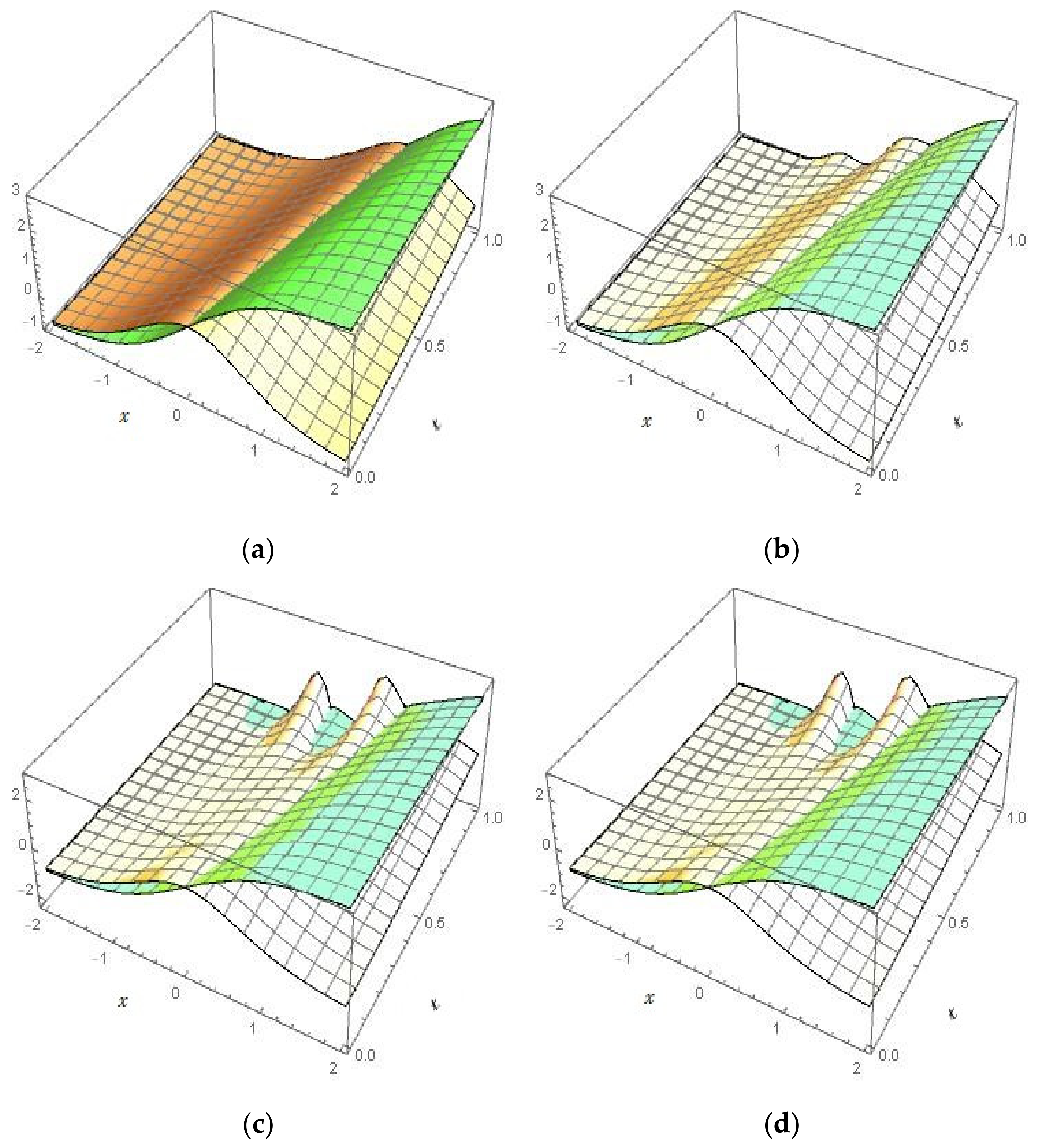
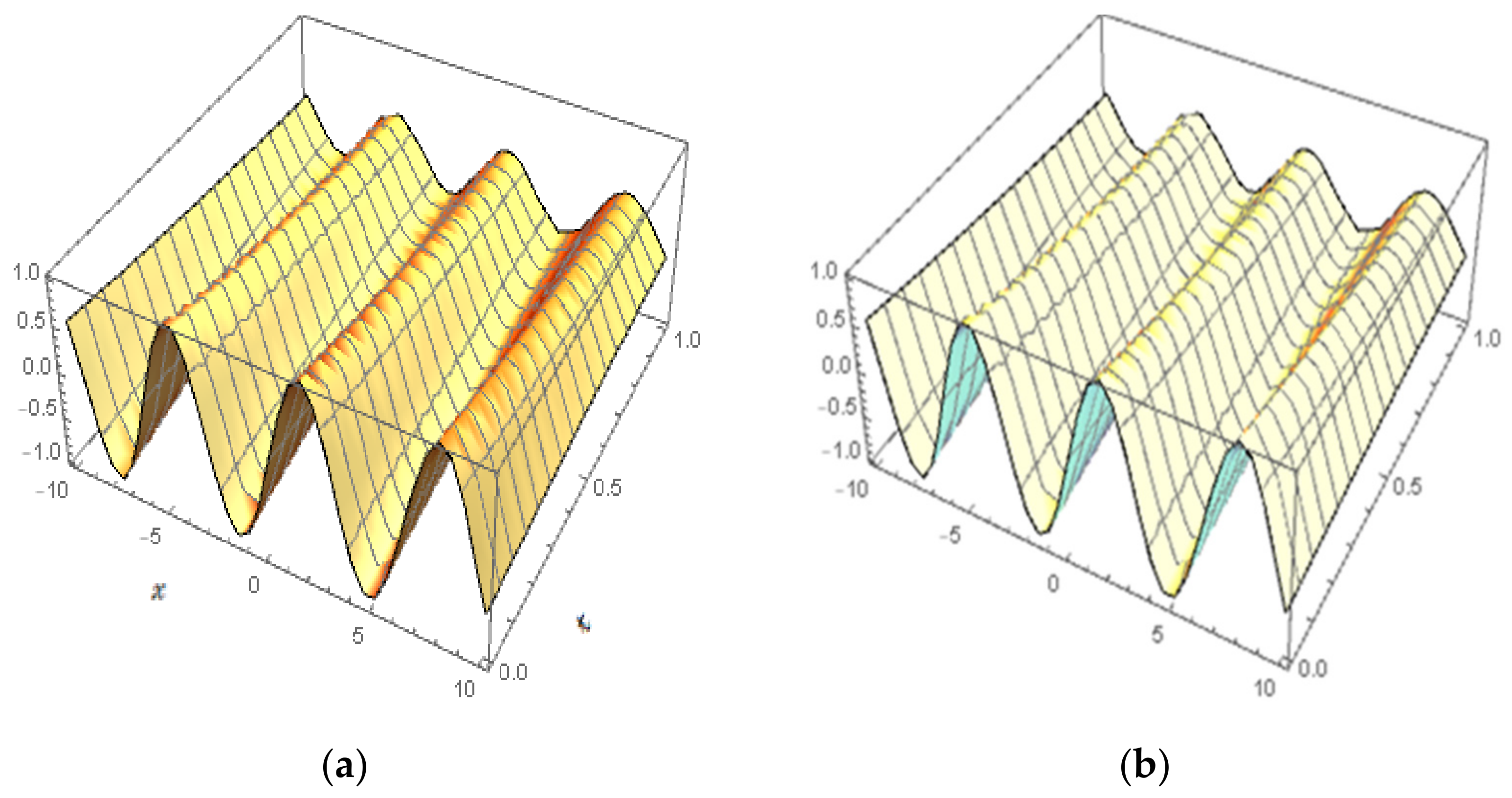
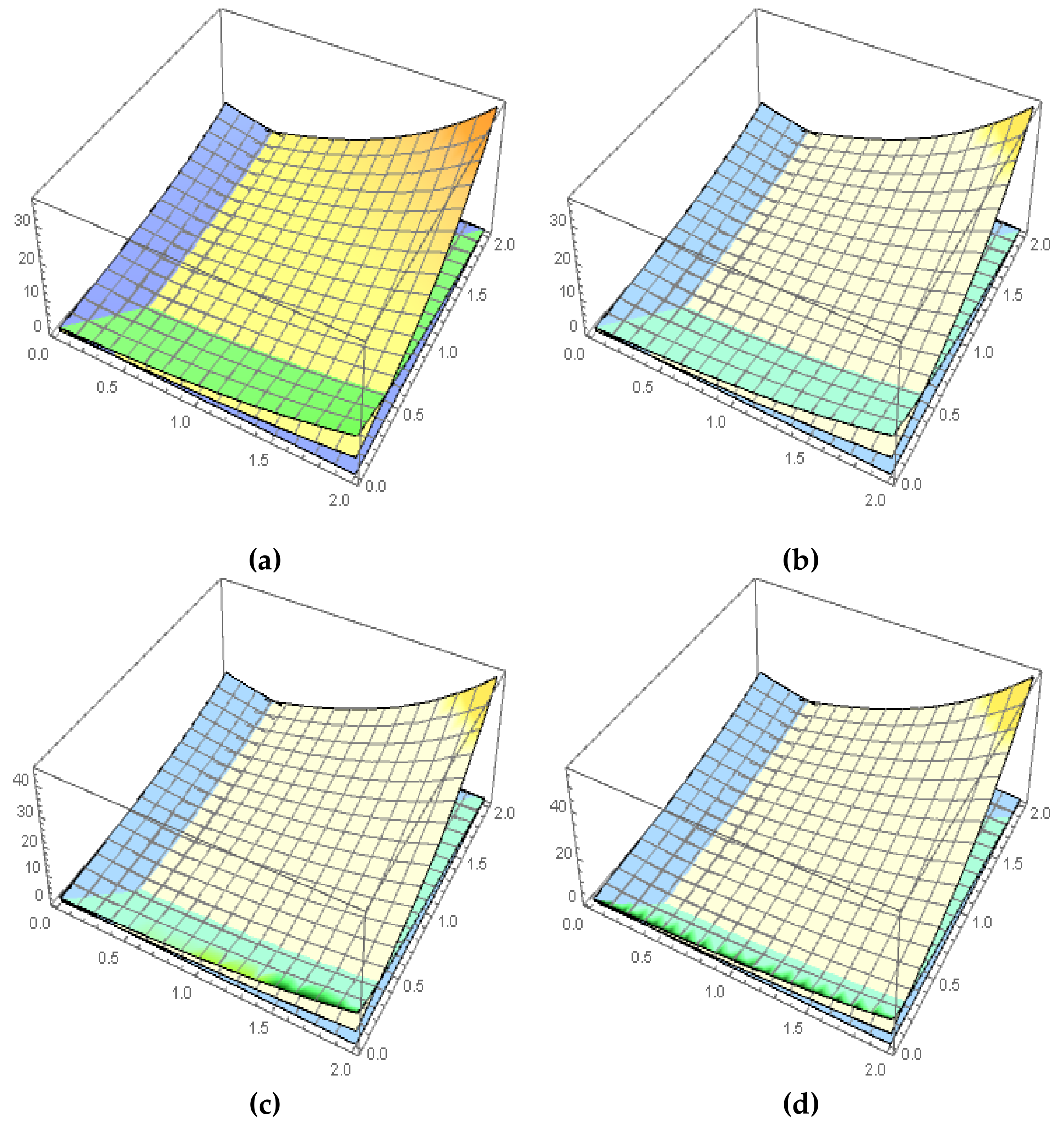
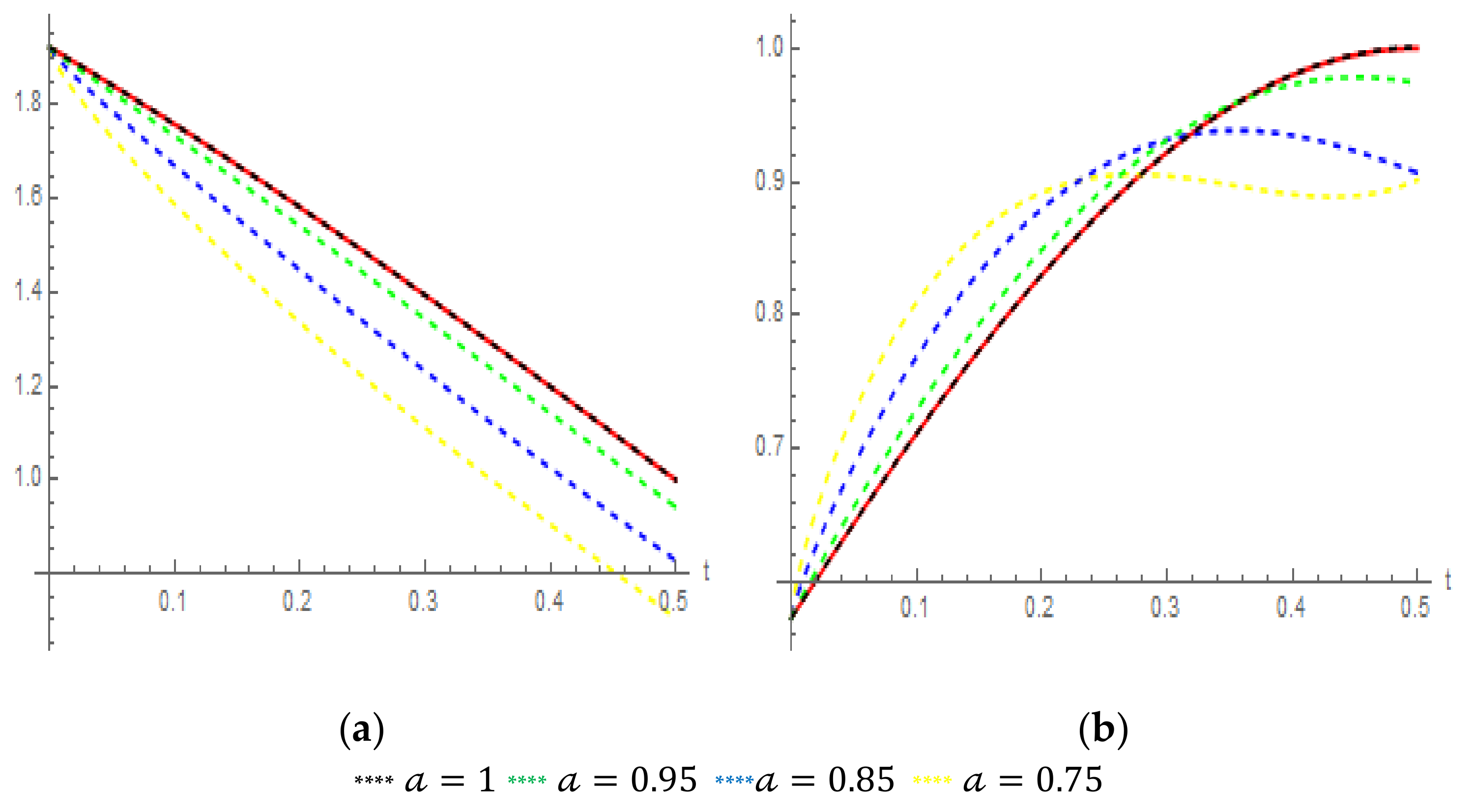
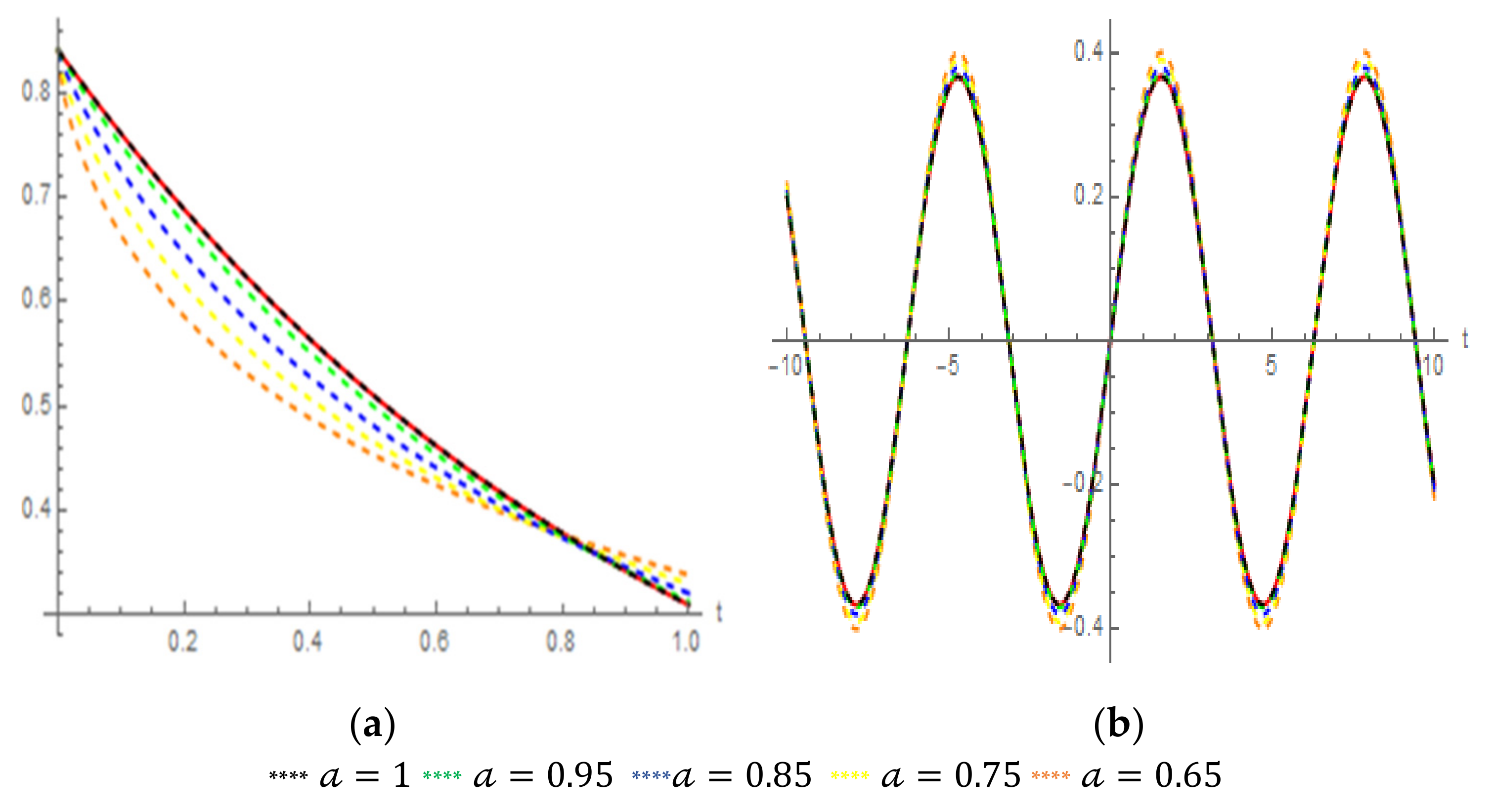
The 3D plots behavior of the approximate solutions of the time-FPDEs (7), (20), and (44) by Laplace RPSM are shown respectively in Figure 1, Figure 2 and Figure 3 at various values of 𝓪   which are compared with the exact solutions on their domains. Obviously, from these figures, it can be deduced that the geometric behaviors almost agree and strongly match each other, particularly when the integer order derivative is considered. From these graphics, we can conclude that the dynamic behaviors match and correspond well with each other, specifically when the standard order derivative is considered. Moreover, Figure 4 and Figure 5 demonstrate the behavior of the obtained Laplace RPS solutions for the systems of the time-FPDEs (7) and (20) at various values of 𝓪   . It is observed from these figures that the Laplace RPSM approximate solutions match with solutions at 𝓪 = 1   , and this reinforces the effectiveness of the proposed method.

6. Conclusions

This investigation of time-FPDEs with initial conditions constructs a proper framework for the mathematical modeling of several fractional problems that appear in physical and engineering applications. The current work has introduced the analytical and approximate solutions for known systems of nonlinear time-FPDEs via applying Laplace RPSM. Three nonlinear time-FPDEs systems, including Broer-Kaup and Burgers’ systems, have been investigated utilizing Caputo-time fractional derivatives. The exact and the Laplace RPS solutions have been displayed numerically and graphically at various values of the fractional order 𝒶 over (0, 1]. The analysis of simulation results revealed that the Laplace RPS solutions are in imminent consistency with each other, as well as with the exact solutions at integer-order of 𝒶, which confirms the performance of the proposed method. Numerical comparisons of the obtained results with the results previously calculated by other numerical methods, such as modified generalized Mittag–Leffler function method MGMLFM [40] and fractional natural decomposition method FNDM [41], have been achieved, which indicates the high accuracy and effectiveness of the Laplace RPSM. Consequently, the analysis of attained results and their simulations confirm that the Laplace RPSM is an easy and systematic, robust, efficient, and suitable instrument to generate analytical and approximate solutions of several fractional physical and engineering problems with fewer computations and iteration steps.

Author Contributions

Conceptualization, H.A. and M.A.; methodology, H.A.; software, H.A.; validation, M.A., A.I. and M.D.; writing—original draft preparation, H.A.; writing—review and editing, A.I. and M.D.; supervision, A.I. and M.D.; funding acquisition, A.I. All authors have read and agreed to the published version of the manuscript.

Funding

Universiti Kebangsaan Malaysia (DIP-2020-001).

Data Availability Statement

Not applicable.

Conflicts of Interest

The authors declare no conflict of interest.

References

  1. Mainardi, F.; Raberto, M.; Gorenflo, R.; Scalas, E. Fractional calculus and continuous-time finance II: The waiting-time distribution. Phys. A Stat. Mech. Its Appl. 2000, 287, 468–481. [Google Scholar] [CrossRef] [Green Version]
  2. He, J.H. Some applications of nonlinear fractional differential equations and their approximations. Bull. Sci. Technol. 1999, 15, 86–90. [Google Scholar]
  3. Caputo, M. Linear models of dissipation whose Q is almost frequency independent—II. Geophys. J. Int. 1967, 13, 529–539. [Google Scholar] [CrossRef]
  4. Oldham, K.B.; Spanier, J. The Fractional Calculus. Integrations and Differentiations of Arbitrary Order; Academic Press: Cambridge, MA, USA, 1974. [Google Scholar]
  5. Podlubny, I. Fractional Differential Equations; Academic Press: Cambridge, MA, USA, 1999. [Google Scholar]
  6. Alabedalhadi, M.; Al-Smadi, M.; Abu Arqub, O.; Baleanu, D.; Momani, S. Structure of optical soliton solution for nonlinear resonant space-time Schrödinger equation in conformable sense with full nonlinearity term. Phys. Scr. 2020, 95, 105215. [Google Scholar] [CrossRef]
  7. Al-Smadi, M.; Abu Arqub, O. Computational algorithm for solving fredholm time-fractional partial integrodifferential equations of Dirichlet functions type with error estimates. Appl. Math. Comput. 2019, 342, 280–294. [Google Scholar] [CrossRef]
  8. Jleli, M.; Kumar, S.; Kumar, R.; Samet, B. Analytical approach for time fractional wave equations in the sense of Yang-Abdel-Aty-Cattani via the homotopy perturbation transform method. Alex. Eng. J. 2020, 59, 2859–2863. [Google Scholar] [CrossRef]
  9. Hasan, S.; Al-Smadi, M.; Dutta, H.; Momani, S.; Hadid, S. Multi-step reproducing kernel algorithm for solving Caputo–Fabrizio fractional stiff models arising in electric circuits. Soft Comput. 2022, 26, 3713–3727. [Google Scholar] [CrossRef]
  10. Hasan, S.; El-Ajou, A.; Hadid, S.; Al-Smadi, M.; Momani, S. Atangana-Baleanu fractional framework of reproducing kernel technique in solving fractional population dynamics system. Chaos Solitons Fract. 2020, 133, 109624. [Google Scholar] [CrossRef]
  11. Liu, Y.; Liu, Z.; Wen, C.F. Existence of solutions for space-fractional parabolic hemivariational inequalities. Discret. Contin. Dyn. Syst. B 2019, 24, 1297. [Google Scholar] [CrossRef] [Green Version]
  12. Li, X.; Li, Y.; Liu, Z.; Li, J. Sensitivity analysis for optimal control problems described by nonlinear fractional evolution inclusions. Fract. Calc. Appl. Anal. 2018, 21, 1439–1470. [Google Scholar] [CrossRef]
  13. Liu, Y.; Liu, Z.; Wen, C.F.; Yao, J.C. Existence of solutions for non-coercive variational-hemivariational inequalities involving the nonlocal fractional p-Laplacian. Optimization 2022, 71, 485–503. [Google Scholar] [CrossRef]
  14. Al-Smadi, M.; Dutta, H.; Hasan, S.; Momani, S. On numerical approximation of Atangana-Baleanu-Caputo fractional integro-differential equations under uncertainty in Hilbert Space. Math. Model. Nat. Phenom. 2021, 16, 41. [Google Scholar] [CrossRef]
  15. Al-Smadi, M.; Abu Arqub, O.; Zeidan, D. Fuzzy fractional differential equations under the Mittag-Leffler kernel differential operator of the ABC approach: Theorems and applications. Chaos Solitons Fract. 2021, 146, 110891. [Google Scholar] [CrossRef]
  16. Al-Smadi, M.; Abu Arqub, O.; Gaith, M. Numerical simulation of telegraph and Cattaneo fractional-type models using adaptive reproducing kernel framework. Math. Methods Appl. Sci. 2021, 44, 8472–8489. [Google Scholar] [CrossRef]
  17. Alabedalhadi, M.; Al-Smadi, M.; Al-Omari, S.; Momani, S. New optical soliton solutions for coupled resonant Davey-Stewartson system with conformable operator. Opt. Quant. Electron. 2022, 54, 392. [Google Scholar] [CrossRef]
  18. Shqair, M.; Farrag, E.A.M.; Al-Smadi, M. Solving Multi-Group Reflected Spherical Reactor System of Equations Using the Homotopy Perturbation Method. Mathematics 2022, 10, 1784. [Google Scholar] [CrossRef]
  19. Shqair, M.; Alabedalhadi, M.; Al-Omari, S.; Al-Smadi, M. Abundant exact travelling wave solutions for a fractional massive hirring model using extended Jacobi elliptic function method. Fract. Fract. 2022, 6, 252. [Google Scholar] [CrossRef]
  20. Wang, G. A (2 + 1)-dimensional sine-Gordon and sinh-Gordon equations with symmetries and kink wave solutions. Nucl. Phys. B 2020, 953, 114956. [Google Scholar] [CrossRef]
  21. Kumar, P.; Baleanu, D.; Erturk, V.S.; Inc, M.; Govindaraj, V. A delayed plant disease model with Caputo fractional derivatives. Adv. Cont. Discr. Mod. 2022, 2022, 11. [Google Scholar] [CrossRef]
  22. Wu, L.; Xie, L.d.; Zhang, J.f. Adomian decomposition method for nonlinear differential-difference equations. Commun. Nonlinear Sci. Numer. Simul. 2009, 14, 12–18. [Google Scholar] [CrossRef]
  23. Odibat, Z.; Momani, S. Application of variational iteration method to nonlinear differential equations of fractional order. Int. J. Nonlinear Sci. Numer. Simul. 2006, 7, 27–34. [Google Scholar] [CrossRef]
  24. Yulita Molliq, R.; Noorani, M.S.M. Solving the fractional Rosenau-Hyman equation via variational iteration method and homotopy perturbation method. Int. J. Differ. Equ. 2012, 2012, 472030. [Google Scholar] [CrossRef] [Green Version]
  25. Xu, H.; Liao, S.-J.; You, X.-C. Analysis of nonlinear fractional partial differential equations with the homotopy analysis method. Commun. Nonlinear Sci. Numer. Simul. 2009, 14, 1152–1156. [Google Scholar] [CrossRef]
  26. Hasan, S.; Al-Smadi, M.; El-Ajou, A.; Momani, S.; Hadid, S.; Al-Zhour, Z. Numerical approach in the Hilbert space to solve a fuzzy Atangana-Baleanu fractional hybrid system. Chaos Solitons Fract. 2021, 143, 110506. [Google Scholar] [CrossRef]
  27. Al-Smadi, M.; Freihat, A.; Khalil, H.; Momani, S.; Ali Khan, R. Numerical multistep approach for solving fractional partial differential equations. Int. J. Comput. Methods 2017, 14, 1750029. [Google Scholar] [CrossRef]
  28. Alaroud, M.; Al-Smadi, M.; Ahmad, R.R.; Din, U.K.S. Computational optimization of residual power series algorithm for certain classes of fuzzy fractional differential equations. Int. J. Differ. Equ. 2018, 2018, 8686502. [Google Scholar] [CrossRef]
  29. Al-Smadi, M.; Abu Arqub, O.S. Momani, Numerical computations of coupled fractional resonant Schrödinger equations arising in quantum mechanics under conformable fractional derivative sense. Phys. Scr. 2020, 95, 075218. [Google Scholar] [CrossRef]
  30. Al-Smadi, M.; Abu Arqub, O.; Hadid, S. Approximate solutions of nonlinear fractional Kundu-Eckhaus and coupled fractional massive Thirring equations emerging in quantum field theory using conformable residual power series method. Phys. Scr. 2020, 95, 105205. [Google Scholar] [CrossRef]
  31. Alaroud, M.; Ahmad, R.R.; Din, U.K.S. An efficient analytical-numerical technique for handling model of fuzzy differential equations of fractional-order. Filomat. 2019, 33, 617–632. [Google Scholar] [CrossRef] [Green Version]
  32. Bataineh, M.; Alaroud, M.; Al-Omari, S.; Agarwal, P. Series Representations for Uncertain Fractional IVPs in the Fuzzy Conformable Fractional Sense. Entropy 2019, 23, 1646. [Google Scholar] [CrossRef]
  33. Freihet, A.; Hasan, S.; Alaroud, M.; Al-Smadi, M.; Ahmad, R.R.; Din, U.K.S. Toward computational algorithm for time-fractional Fokker–Planck models. Adv. Mech. Eng. 2019, 11, 1687814019881039. [Google Scholar] [CrossRef]
  34. Al-Smadi, M. Fractional residual series for conformable time-fractional Sawada–Kotera–Ito, Lax, and Kaup–Kupershmidt equations of seventh order. Math. Methods Appl. Sci. 2021, 1–22. [Google Scholar] [CrossRef]
  35. Alaroud, M.; Al-smadi, M.; Ahmad, R.R.; Salma Din, U.K. Numerical computation of fractional Fredholm integro-differential equation of order 2β arising in natural sciences. J. Phys. Conf. Ser. 2019, 1212, 012022. [Google Scholar] [CrossRef]
  36. Hanna, J.; Rowland, J. Fourier Series, Transforms, and Boundary Value Problems; Wiley: New York, NY, USA, 1990. [Google Scholar]
  37. El-Ajou, A. Adapting the Laplace transform to create solitary solutions for the nonlinear time-fractional dispersive PDEs via a new approach. Eur. Phys. J. Plu. 2021, 136, 229. [Google Scholar] [CrossRef]
  38. Alaroud, M.; Tahat, N.; Al-Omari, S.; Suthar, D.L.; Gulyaz-Ozyurt, S. An Attractive Approach Associated with Transform Functions for Solving Certain Fractional Swift-Hohenberg Equation. J. Funct. Spaces 2021, 2021, 3230272. [Google Scholar] [CrossRef]
  39. Aljarrah, H.; Alaroud, M.; Ishak, A.; Darus, M. Approximate solution of nonlinear time-fractional PDEs by Laplace residual power series method. Mathematics 2022, 10, 1980. [Google Scholar] [CrossRef]
  40. Ali, H.M.; Ahmad, H.; Askar, S.; Ameen, I.G. Efficient approaches for solving systems of nonlinear time-fractional partial differential equations. Fract. Fract. 2022, 6, 32. [Google Scholar] [CrossRef]
  41. Rawashdeh, M.S.; Al-Jammal, H. New approximate solutions to fractional nonlinear systems of partial differential equations using the FNDM. Adv. Differ. Equ. 2016, 2016, 235. [Google Scholar] [CrossRef]
Figure 1. 3D-Surfaces plot of the exact solution of U 𝓍 , 𝓉 and V 𝓍 , 𝓉 , and the 7 t h approximate solution U 7 𝓍 , 𝓉 and V 7 𝓍 , 𝓉 , for IVP (7), with 𝓉 0 , 1 , and   𝓍   2 , 2 , at various values of 𝓪 . (a) U 𝓍 , 𝓉 , V 𝓍 , 𝓉 . (b) U 7 𝓍 , 𝓉 , V 7 𝓍 , 𝓉 : 𝓪 = 1 . (c) U 7 𝓍 , 𝓉 , V 7 𝓍 , 𝓉 : 𝓪 = 0.97 . (d) U 7 𝓍 , 𝓉 , V 7 𝓍 , 𝓉 : 𝓪 = 0.87 .
Fractalfract 06 00650 g001
Figure 2. 3D-Surfaces plot of exact solutions U 𝓍 , 𝓉 , V 𝓍 , 𝓉 , and the 7 t h approximate solutions U 7 𝓍 , 𝓉 , V 7 𝓍 , 𝓉 , for system (20), with 𝓉 0 , 1 , and 𝓍 10 , 10 , at various values of 𝓪 . (a) U 𝓍 , 𝓉 , V 𝓍 , 𝓉 .   b U 7 𝓍 , 𝓉 , V 7 𝓍 , 𝓉 : 𝓪 = 1 .     c U 7 𝓍 , 𝓉 , V 7 𝓍 , 𝓉 : 𝓪 = 0.95 .   d   U 7 𝓍 , 𝓉 , V 7 𝓍 , 𝓉 : 𝓪 = 0.85 .
Fractalfract 06 00650 g002aFractalfract 06 00650 g002b
Figure 3. 3D-Surfaces Plot of Exact solutions of U , V ,   W the 7 t h approximate solution U 7 , V 7 ,   W 7 , for system (33), with 𝓉 0 , 2 , and 𝓍 0 , 2 and 𝓎 = 0.4 , at various values of 𝓪 . (a) U , V ,   W .   (b) U 7 , V 7 ,   W 7   :   𝓪 = 1 .   (c) U 7 , V 7 ,   W 7 : 𝓪 = 0.8 . (d) U 7 , V 7 ,   W 7 : 𝓪 = 0.6 .
Fractalfract 06 00650 g003
Figure 4. (a) 2D-Plots of exact solutions U (𝓍,𝓉), and the 7-th approximate solutions U 7 (𝓍,𝓉) and V 7 (𝓍,𝓉), for system (7), with 𝓉 ∈ [0, 0.5], and 𝓍 = 1, at various values of 𝒶. (b) 2D-Plots of exact solutions V (𝓍,𝓉), and the 7-th approximate solutions V 7 (𝓍,𝓉), for system (7), with 𝓉 ∈ [0, 0.5], and 𝓍 = 1, at various values of 𝒶.
Fractalfract 06 00650 g004
Figure 5. Plots of exact solutions ( U (𝓍,𝓉), V (𝓍,𝓉)), and the 7-th approximate solutions ( U 7 (𝓍,𝓉), V 7 (𝓍,𝓉)), for system (20) at various values of 𝒶. (a) 𝓉 ∈ [0, 1], and 𝓍 = 1. (b) 𝓍 ∈ [−10, 10], and 𝓉 = 1.
Fractalfract 06 00650 g005
Table 1. Numerical results for Example 1 at 𝓍 = 1 ,   𝓪 = 1 ,   and   n = 7 .
Numerical   Results   of   U 𝓍 , 𝓉  
𝓉 i   U 𝓍 , 𝓉 U 7 𝓍 , 𝓉 U U 7  
0.1 2.4325957403980487 2.4325957405419616 1.439128816116408 × 10 10
0.2 2.3280735405356980 2.3280735789915883 3.845589047202225 × 10 8
0.3 2.2087355542343268 2.2087365789980504 1.024763723656008 × 10 6
0.4 2.0740991339960706 2.0741097277878920 1.059379182155595 × 10 5
0.5 1.9242343145200196 1.9242993140796738 6.499955965422188 × 10 5
0.6 1.7598979245104498 1.7601838692172310 2.859447067811161 × 10 4
0.7 1.5826252249031816 1.5836225257595018 9.973008563202157 × 10 4
0.8 1.3947506404498080 1.3976783358533416 2.927695403533548 × 10 3
0.9 1.1993359892499116 1.2068540917157446 7.518102465833065 × 10 3
Numerical Results of V 𝓍 , 𝓉
𝓉 i V 𝓍 , 𝓉 V 7 𝓍 , 𝓉 V V 7
0.1 0.0261652777033167 0.0261652782859831 5.82666359605355 × 10 10
0.2 0.11811033546448813 0.11811018874091550 1.46723572624907 × 10 7
0.3 0.26947917996491720 0.26947552093723215 3.659027685065652 × 10 6
0.4 0.42315552517444555 0.42312041684151236 3.510833293318694 × 10 5
0.5 0.57289546593185480 0.57269750532341330 1.497960608441461 × 10 4
0.6 0.71127757216235540 0.71048682802189810 7.907441404573223 × 10 4
0.7 0.83027392365325850 0.82780654822770770 2.467375425550755 × 10 3
0.8 0.92208596593223320 0.91572529863721930 6.360667295013944 × 10 3
0.9 0.98013258169487960 0.96613158040482160 1.400100129005799 × 10 3
Table 2. Numerical results for Example 2 at x = 10 ,   𝓪 = 1 ,   and   n = 7 .
Numerical   Results   of   U 𝓍 , 𝓉  
𝓉 i   U 𝓍 , 𝓉 U 7 𝓍 , 𝓉 Abs. Error
0.2 0.4454068138087739 0.4454068137749855 3.378847202029078 × 10 11
0.4 0.3646682560957220 0.3646682476310534 8.464668632690575 × 10 9
0.6 0.2985651159368848 0.2985649035620645 2.123748202298436 × 10 7
0.8 0.2444444422138206 0.2444423647493085 2.077464512112437 × 10 6
1 0.2001341822594486 0.2001220515057324 1.213075371614413 × 10 5
Numerical Results of V 𝓍 , 𝓉
𝓉 i V 𝓍 , 𝓉 V 7 𝓍 , 𝓉 Abs. Error
0.2 0.4454068138087739 0.4454068137749855 3.378847202029078 × 10 11
0.4 0.3646682560957220 0.3646682476310534 8.464668632690575 × 10 9
0.6 0.2985651159368848 0.2985649035620645 2.123748202298436 × 10 7
0.8 0.2444444422138206 0.2444423647493085 2.077464512112437 × 10 6
1 0.2001341822594486 0.2001220515057324 1.213075371614413 × 10 5
Table 3. Numerical results for Example 3 at different values of 𝓍 , 𝓎 = 0.4 , 𝓪 = 1 ,   and   n = 7 .
Numerical   Results   of   U 𝓍 , 𝓎 , 𝓉
𝓍 i   𝓉 i   U 𝓍 , 𝓎 , 𝓉 U 7 𝓍 , 𝓎 , 𝓉 U U 7  
0.5 0.3 1.8221188003905090 1.8221187965176793 3.872829834605795 × 10 9
0.6 1.3498588075760032 1.3498578473967784 9.601792247959650 × 10 7
0.9 1.0 0.9999761481976381 2.385180236186279 × 10 5
1 0.3 3.0041660239464334 3.0041660175612160 6.385217243831676 × 10 9
0.6 2.2255409284924680 2.2255393454245560 1.583067911870017 × 10 6
0.9 1.6487212707001284 1.6486819457262294 3.932497389902423 × 10 5
1.5 0.3 4.9530324243951150 4.9530324138676710 1.052744380558579 × 10 8
0.6 3.6692966676192444 3.6692940575815050 2.610037739270154 × 10 6
0.9 2.718281828459045 2.718216992538108 6.483592093697865 × 10 5
Numerical Results of V 𝓍 , 𝓎 , 𝓉
𝓍 i 𝓉 i V 𝓍 , 𝓎 , 𝓉 V 7 𝓍 , 𝓎 , 𝓉 V V 7
0.5 0.3 1.4918246976412703 1.4918246957811063 1.860164022815524 × 10 9
0.6 2.0137527074704766 2.0137522144484308 4.930220458554402 × 10 7
0.9 2.7182818284590450 2.7182687338653180 1.309459372711430 × 10 5
1 0.3 2.4596031111569500 2.4596031080900580 3.066891629543988 × 10 9
0.6 3.3201169227365480 3.3201161098806145 8.128559336739727 × 10 7
0.9 4.4816890703380645 4.4816674810028550 2.158933520934880 × 10 5
1.5 0.3 4.0551999668446745 4.0551999617882260 5.056448593165896 × 10 9
0.6 5.4739473917272010 5.4739460515543330 1.340172867791977 × 10 6
0.9 7.3890560989306500 7.3890205041344710 3.559479617898376 × 10 5
Numerical Results of W 𝓍 , 𝓎 , 𝓉
𝓍 i 𝓉 i W 𝓍 , 𝓎 , 𝓉 W 7 𝓍 , 𝓎 , 𝓉 W W 7
0.5 0.3 1.2214027581601699 1.2214027566371966 1.52297330302531 × 10 9
0.6 1.6487212707001282 1.6487208670478177 4.03652310465574 × 10 7
0.9 2.2255409284924674 2.2255302075458845 1.07209465829427 × 10 5
1 0.3 0.7408182206817179 0.7408182197579880 9.2372987037236 × 10 10
0.6 1.0 0.9999997551724980 2.44827502049461 × 10 7
0.9 1.3498588075760030 1.3498523049931992 6.50258280376903 × 10 6
1.5 0.3 0.4493289641172216 0.4493289635569510 5.60270607685710 × 10 10
0.6 0.6065306597126334 0.6065305112172470 1.48495386431690 × 10 7
0.9 0.8187307530779818 0.8187268090621439 3.94401583792003 × 10 6
Table 4. Numerical results of approximated solutions, at n   =   7 ,    𝓍 = 1, and different values of 𝒶, for Example 1.
U 7 (𝓍,𝓉)
𝓉i𝒶 = 1𝒶 = 0.97𝒶 = 0.87𝒶 = 0.77
0.152.38213894343579102.36604882210417702.31649856735528342.2494580999988480
0.302.20873657899805042.17988404194171362.09466914785703471.9890784760486064
0.452.00106802012981031.96054981086795091.84754909835536421.7270938997910783
0.601.76018386921723171.71106108439648201.58716114810741641.4930439371551603
0.751.49157844419139851.44045463656961431.33619124668197961.3308640595516880
0.901.20685409171574461.16532852414006421.12849344411488441.2968610082469043
V 7 (𝓍,𝓉)
𝓉i𝒶 = 1𝒶 = 0.97𝒶 = 0.87𝒶 = 0.77
0.150.04484596090082980.06638699880978890.1296414678807820.2067709053195330
0.300.26947552093723190.30093126502847300.38258278261974650.4565703174103681
0.450.49887123982751660.52983701509168160.59145242449456690.6089345684206415
0.600.71048682802189810.72694689723144790.72682683742870520.6726093727343672
0.750.87598244531398460.86236112829113880.77448584554374310.7307371590702421
0.900.96613158040482160.91124501352223430.75966241765392460.9841962235906878
Table 5. Numerical results of approximated solutions, at n = 7, 𝓍 = 10, and different values of 𝒶, for Example 2.
U 7 (𝓍,𝓉)
𝓉i𝒶 = 1𝒶 = 0.95𝒶 = 0.85𝒶 = 0.75
0.2−0.4454068138087739−0.4366187365008558−0.41802625689971980−0.3985414981473607
0.4−0.3646682560957220−0.3565811645027616−0.34129966933185546−0.3275638100454310
0.6−0.2985651159368848−0.2934671682315440−0.28497017140893940−0.2786635555415501
0.8−0.2444444422138206−0.2429390773523567−0.24160764152557102−0.2420836601179408
1.0−0.2001341822594486−0.2021160815904085−0.20726098237141660−0.2132493814323069
V 7 (𝓍,𝓉)
𝓉i𝒶 = 1𝒶 = 0.95𝒶 = 0.85𝒶 = 0.75
0.2−0.4454068138087739−0.4366187365008558−0.41802625689971980−0.3985414981473607
0.4−0.3646682560957220−0.3565811645027616−0.34129966933185546−0.3275638100454310
0.6−0.2985651159368848−0.2934671682315440−0.28497017140893940−0.2786635555415501
0.8−0.2444444422138206−0.2429390773523567−0.24160764152557102−0.2420836601179408
1.0−0.2001341822594486−0.2021160815904085−0.20726098237141660−0.2132493814323069
Table 6. Numerical results of approximated solutions, at y = 0.4 and different values of 𝓍, 𝓉, and 𝒶, with n   =   7 for Example 3.
U 7 (𝓍,𝓎,𝓉)
𝓍i𝓉i𝒶 = 1𝒶 = 0.95𝒶 = 0.75𝒶 = 0.55
0.50.31.822118796517671.7818543549229401.6241658153249871.485973706352699
0.61.349857847396771.32681020195098821.2598807922279961.224207523196436
0.90.999976148197631.00125590867025931.0258447213131541.048930393543767
10.33.004166017561212.9377811762511182.6777967268703222.449956457364802
0.62.225539345424552.1875402021385262.0771922606928272.018376983245085
0.91.648681945726221.6507919140388411.6913320124644421.729393851319466
1.50.34.953032413867674.84358231394765954.4149404222022814.039295323546481
0.63.669294057581503.60664406177744653.4247110635379493.327741064567730
0.92.718216992538102.72169574217561432.7885350647661802.851288428088421
V 7 (𝓍,𝓎,𝓉)
𝓍i𝓉i𝒶 = 1𝒶 = 0.95𝒶 = 0.75𝒶 = 0.55
0.50.31.491824695781111.5337767163298841.7639063480076792.173624234307866
0.62.013752214448432.0905174670117992.5008221664199683.2070987754409066
0.92.718268733865322.8365533351812823.4639094781914944.5195588991940581
10.32.459603108090052.5287702967176762.9081899154832453.5837005096126577
0.63.320116109880613.4466806146325074.1231587000149785.2876119683057565
0.94.481667481002854.6766858191887715.7110212364740987.4514928912833001
1.50.34.055199961788224.1692373769131074.7947945728928345.9085232580172781
0.65.473946051554335.6826156426544066.7979394511869848.7177983233542732
0.97.389020504134477.7105513864781829.41588218999499412.285434828329576
W 7 (𝓍,𝓎,𝓉)
𝓍i𝓉i𝒶 = 1𝒶 = 0.95𝒶 = 0.75𝒶 = 0.55
0.50.31.221402756637191.2557501660142391.4441643726633611.7796130062634311
0.61.648720867047811.7115709400892452.0475000156271312.6257503956122070
0.92.225530207545882.3223734482588332.8360092156736813.7003018611174463
10.30.740818219757980.7616509766268660.87592996968498961.0793898507221418
0.60.999999755172491.0381202514373021.24187153523995121.5925981196913803
0.91.349852304993191.4085906996715331.72012654053366632.2443465289594501
1.50.30.449328963556950.461964669324270.53127838237510360.6546830382456215
0.60.606530511217240.629651760965310.75323316154742840.9659595881935124
0.90.818726809062150.854353446336851.04330948541909431.3612649808335340
Table 7. Numerical comparisons for Example 1 at 𝒶 = 1 and different values of 𝓍 and 𝓉.
U U 2
𝓍 = −1𝓍 = 0.5𝓍 = 1
𝓉iLRPSMMGMLFM [40]LRPSMMGMLFM [40]LRPSMMGMLFM [40]
0.0035.59911 × 10−94.51907 × 10−55.11357 × 10−94.53038 × 10−55.59013 × 10−93.28798 × 10⁻⁵
0.0064.48282 × 10−81.79812 × 10−44.11223 × 10−81.80805 × 10−44.46846 × 10−81.2751 × 10⁻⁴
0.0091.51413 × 10−74.02448 × 10−41.3951 × 10−74.05897 × 10−41.50686 × 10−72.78165 × 10⁻⁴
V V 2
𝓍 = −1𝓍 = 0.5𝓍 = 1
𝓉iLRPSMMGMLFM [40]LRPSMMGMLFM [40]LRPSMMGMLFM [40]
0.0035.94837 × 10−91.3969 × 10−53.55919 × 10−82.14755 × 10−56.02338 × 10−91.25863 × 10⁻⁴
0.0064.72882 × 10−85.5459 × 10−52.84908 × 10−78.62386 × 10−54.84885 × 10−84.93352 × 10⁻⁴
0.0091.58592 × 10−71.23872 × 10−49.62139 × 10−71.94798 × 10−41.64669 × 10−71.08802 × 10⁻³
Table 8. Numerical comparisons for Example 1 at different values of 𝓍, 𝒶, and 𝓉 for the function U .
𝒶 = 1
(𝓍,𝓉i) U (𝓍,𝓉i) LRPSMMGMLFM [40]
(−0.5, 0.003)0.07105354590.07105354080.0710849
(−0.5, 0.006)0.06635451990.06635447970.0664763
(0.5, 0.003)1.91950909151.919509086361.91955
(0.5, 0.006)1.91477081581.914770774691.91495
𝒶 = 0.9
(𝓍,𝓎,𝓉i) U (𝓍,𝓎,𝓉i)LRPSMMGMLFM [40]
(−0.5, 0.003)0.07105354590.067189858100.0671357
(−0.5, 0.006)0.06635451990.059895889860.0598679
(0.5, 0.003)1.91950909151.915838607831.91561
(0.5, 0.006)1.91477081581.909880837471.90838
𝒶 = 0.8
(𝓍,𝓎,𝓉i) U (𝓍,𝓎,𝓉i)LRPSMMGMLFM [40]
(−0.5, 0.003)0.07105354590.060668681200.0600753
(−0.5, 0.006)0.06635451990.049760893520.0489784
(0.5, 0.003)1.91950909151.909950395331.90859
(0.5, 0.006)1.91477081581.898763008511.8977
Table 9. Numerical comparisons for Example 2 at different values of 𝓍, 𝒶, and 𝓉 for the function U .
𝒶 = 1
(𝓍,𝓉i) U (𝓍,𝓉i) LRPSMMGMLFM [40]
(−10, 0.2)0.44540681380.44540681370.4454068
(−10, 0.4)0.36466825700.36466824760.3646684
(−5, 0.2)0.78510079350.78510079350.7851008
(−5, 0.4)0.64278616390.64278614900.6427865
𝒶 = 0.9
(𝓍,𝓎,𝓉i) U (𝓍,𝓎,𝓉i)LRPSMMGMLFM [40]
(−10, 0.2)0.44540681380.427472543280.4274714
(−10, 0.4)0.36466825700.348778612880.3487726
(−5, 0.2)0.78510079350.753496656290.7534867
(−5, 0.4)0.64278616390.614775257330.6147676
𝒶 = 0.75
(𝓍,𝓎,𝓉i) U (𝓍,𝓎,𝓉i)LRPSMMGMLFM [40]
(−10, 0.2)0.44540681380.398551498150.3985421
(−10, 0.4)0.36466825700.327663810080.3275878
(−5, 0.2)0.78510079350.702503174230.7024943
(−5, 0.4)0.64278616390.577493639470.5774259
Table 10. Numerical comparisons for Example 3 at different values of 𝓍, 𝒶, and 𝓉 for the function U .
𝒶 = 1
(𝓍,𝓎,𝓉i) U (𝓍,𝓎,𝓉i) LRPSMMGMLFM [40]FNDM [41]
(0.5, 0.4, 0.3)1.82211881.82211881.82211891.82217
(0.5, 0.4, 0.6)1.34985881.34985781.34987151.35131
(0.5, 0.4, 0.9)1.00000000.99997611.000211.0105
(1, 0.4, 0.3)3.00416603.00416603.00416623.00424
(1, 0.4, 0.6)2.22554002.22553942.2255622.22793
(1, 0.4, 0.9)1.64872001.64868201.6490671.66603
(1.5, 0.4, 0.3)4.95303004.95303244.95303274.95316
(1.5, 0.4, 0.6)3.66930003.66929403.66933123.6323
(1.5, 0.4, 0.9)2.71828002.71821692.7188512.74682
𝒶 = 0.9
(𝓍,𝓎,𝓉i) U (𝓍,𝓎,𝓉i)LRPSMMGMLFM [40]FNDM [41]
(0.5, 0.4, 0.3)1.82211881.74158231.741581.74178
(0.5, 0.4, 0.6)1.34985881.30632221.30639961.31047
(0.5, 0.4, 0.9)1.00000001.00484841.00584451.02931
(1, 0.4, 0.3)3.00416602.87138382.8713852.8717
(1, 0.4, 0.6)2.22554002.15376112.15388892.1606
(1, 0.4, 0.9)1.64872001.65671491.65835721.69705
(1.5, 0.4, 0.3)4.95303004.73411164.73411434.73464
(1.5, 0.4, 0.6)3.66930003.55095183.55116243.56223
(1.5, 0.4, 0.9)2.71828002.73146112.73416892.79796
𝒶 = 0.75
(𝓍,𝓎,𝓉i) U (𝓍,𝓎,𝓉i)LRPSMMGMLFM [40]FNDM [41]
(0.5, 0.4, 0.3)1.82211881.62416581.62418971.6256
(0.5, 0.4, 0.6)1.34985881.25988081.26079141.27791
(0.5, 0.4, 0.9)1.00000001.02584471.0334971.10414
(1, 0.4, 0.3)3.00416602.67779672.67783622.68017
(1, 0.4, 0.6)2.22554002.07719222.07869352.10692
(1, 0.4, 0.9)1.64872001.69133201.70394861.82042
(1.5, 0.4, 0.3)4.95303004.41494044.41500554.41885
(1.5, 0.4, 0.6)3.66930003.42471113.42718633.47372
(1.5, 0.4, 0.9)2.71828002.78853512.8093363.00136
Publisher’s Note: MDPI stays neutral with regard to jurisdictional claims in published maps and institutional affiliations.