Article

Sensitivity of Fractional-Order Recurrent Neural Network with Encoded Physics-Informed Battery Knowledge

1
School of Vehicle and Mobility, Tsinghua University, Beijing 100084, China
2
Department of Engineering, University of California, Merced, CA 95343, USA
*
Authors to whom correspondence should be addressed.
Fractal Fract. 2022, 6(11), 640; https://doi.org/10.3390/fractalfract6110640
Submission received: 26 September 2022 / Revised: 27 October 2022 / Accepted: 30 October 2022 / Published: 2 November 2022
(This article belongs to the Special Issue Advances in Fractional Order Systems and Robust Control)

Abstract

:
In the field of state estimation for the lithium-ion battery (LIB), model-based methods (white box) have been developed to explain battery mechanism and data-driven methods (black box) have been designed to learn battery statistics. Both white box methods and black box methods have drawn much attention recently. As the combination of white box and black box, physics-informed machine learning has been investigated by embedding physic laws. For LIB state estimation, this work proposes a fractional-order recurrent neural network (FORNN) encoded with physics-informed battery knowledge. Three aspects of FORNN can be improved by learning certain physics-informed knowledge. Firstly, the fractional-order state feedback is achieved by introducing a fractional-order derivative in a forward propagation process. Secondly, the fractional-order constraint is constructed by a voltage partial derivative equation (PDE) deduced from the battery fractional-order model (FOM). Thirdly, both the fractional-order gradient descent (FOGD) and fractional-order gradient descent with momentum (FOGDm) methods are proposed by introducing a fractional-order gradient in the backpropagation process. For the proposed FORNN, the sensitivity of the added fractional-order parameters are analyzed by experiments under the federal urban driving schedule (FUDS) operation conditions. The experiment results demonstrate that a certain range of every fractional-order parameter can achieve better convergence speed and higher estimation accuracy. On the basis of the sensitivity analysis, the fractional-order parameter tuning rules have been concluded and listed in the discussion part to provide useful references to the parameter tuning of the proposed algorithm.

1. Introduction

As the main energy source and energy storage device, the lithium-ion battery (LIB) and its management have drawn much attention recently. For battery management, safety [1], durability [2], and heterogeneity [3] are the three aspects to be investigated, and the state estimation is the basic function for the three aspects [4,5]. Among the state-of-art literature, the estimation of the state of charge (SOC) [6], state of health (SOH) [7], and remaining useful life (RUL) [8] have been realized by various model-based methods and data-driven methods [9,10]. Model-based methods, especially the electrochemical model [11], can describe inner reactions and lithium concentration changes, such as a loss of lithium inventory (LLI) and loss of active material (LAM) [12,13]. The fractional-order element, also called a Warburg element, has been introduced into the equivalent circuit model (ECM) to construct a fractional-order model (FOM) [14,15]. The FOM can reflect diffusion dynamics in the electrochemical impedance spectrum (EIS), such as the charge transfer reaction and double layer effects in the mid-frequency, and the solid diffusion dynamics in the low-frequency [16,17]. However, the computation burden and complexity of partial derivative equations (PDEs) limit the application of model-based methods in realistic situations. The data-driven method provides a new estimation pattern and replacement for the traditional model-based methods [18]. For realistic battery data with unstable quality [19], data-driven methods are usually designed with a machine learning (ML) algorithm. Among the ML algorithm, neural networks (NNs) are the mainly investigated direction [20], such as the deep neural network (DNN) [21], long short term memory (LSTM) [22], and gated recurrent unit (GRU) [23]. However, the inner battery knowledge cannot be mapped and learned by the state-of-art algorithms due to the lack of interpretability. Hence, current algorithms need to be enhanced to learn the battery’s inner information.
As presented above, model-based methods (white box) and data-driven methods (black box) have been developed independently in two different directions. Hence, physics-informed machine learning has been proposed to combine the advantages of the model-based method and data-driven method, by encoding a physical law of the predicted object. The embedded physics information in ML algorithms were mainly concluded into an observational bias, inductive bias, and learning bias [24]. In this work, we take the advantages of the fractional-order recurrent neural network (FORNN) and fractional-order gradients, which have been investigated theoretically to process time-series data [25,26]. A fractional-order recurrent neural network encoded with physics-informed knowledge of LIB is proposed, called FORNN with PIBatKnow. With encoding battery physical laws, the neural network can be informed by battery knowledge, which acts as a part of the states feedback, the network loss function, and the gradient in backpropagation. The proposed algorithm applies the widely used PDEs to reflect battery physics meanings, which are included in the modeling of LIBs, such as an electrochemical model and ECMs [27,28]. Then, PDEs with physics meanings of the battery are embedded into the network framework; thus, it serves as the representation of battery dynamic characteristic and convergence constraints for network update. Enhanced by physics-informed battery knowledge, nine key fractional-order parameters have been added, and this paper focuses on the sensitivity of the fractional-order parameters to the performance of the proposed FORNN with PIBatKnow. Experiments under dynamic operation conditions are conducted to analyze the sensitivity, and several conclusions have been made in the discussion part to provide useful instructions to the parameter tuning of the proposed algorithm.

2. Preliminaries

2.1. Fractional-Order Derivative

2.1.1. Fractional-Order Derivative Definitions

Fractional calculus is generalized beyond integer calculus by introducing the fractional order α , and many definitions of the fractional operator has been developed in the literature. Three commonly used definitions for fractional derivatives are Riemann-Liouville (R-L), Grünwald-Letnikov (G-L), and Caputo [29]. The R-L definition has too complicated initial conditions to calculated in application, thus this work considers the G-L definition and Caputo definition.
Definition 1
(Grünwald-Letnikov (G-L) Derivative [30]).
G L D t α f ( t ) = lim h 0 h α j = 0 [ t t 0 h ] ( 1 ) j α j f ( t j h ) ,
where G L D t α represents the fractional operator in G-L definition, f ( t ) is a certain integrable function in [ a , b ] , [ t t 0 h ] represents the approximate recursive terms of integer order parts, α j = α ! / j ! ( α j ) ! represents the coefficients of the approximate recursive terms.
Lemma 1 (Finite form of Grünwald-Letnikov Derivative).
If the infinite form in (1) is limited as finite terms L, G L D t α can be discretized as [31]
Δ α f ( x ) = j = 0 L ( 1 ) j α j f ( k j ) ,
where the sum formula in the right side only selects L finite terms of f ( k j ) , j = 0 , 1 , , L , which are the discrete values in the L previous sampling moments.
Definition 2
(Caputo Derivative [30]).
C D t α f ( t ) = 1 Γ ( n α ) t 0 t f ( n ) ( τ ) ( t τ ) α n + 1 d τ , t > t 0 ,
where C D x α represents the fractional operator in Caputo definition, α ( n 1 , n ) , Γ ( · ) is the Gamma function.
Lemma 2.
If f ( x ) is smooth with finite fractional-order derivative, Caputo derivative in (3) can be discretized as [32]
x 0 C D x α f ( x ) = i = n f ( i ) ( x 0 ) Γ ( i + 1 α ) ( x x 0 ) i α .
Lemma 3.
In (4), if f ( x ) = ( x x 0 ) λ , (4) can be deduced as [33]
x 0 C D x α ( x x 0 ) λ = Γ ( λ + 1 ) Γ ( λ α + 1 ) ( x x 0 ) λ α ,
where λ α + 1 > 0 .
The G-L definition in (2) has a discrete implement form for application, and the Caputo definition in (5) holds a simple form for quadratic function, which can apply the fractional-order chain rule. As more general forms of the derivative than the integer-order one, both the G-L definition and Caputo definition can transfer into the integer-order derivative when α = 1 . Hence, we employ G-L derivative for the fractional-order state feedback and fractional-order constraints, then the Caputo derivative for backpropagation with the fractional-order gradient in this work.

2.1.2. Fractional-Order Gradient

The gradient usually works as the iteration direction to search the optimal minimum point of an unconstrained convex optimization problem [34].
min x f ( x ) ,
where f ( x ) is a smooth convex function with a unique global extreme point x * . Gradient in continuous form can be presented as
x ˙ = ρ f ( x ) ,
where ρ > 0 is the iteration step size, and f ( x ) is the gradient of f ( x ) at x. Equation (7) can be discretized as
x k + 1 = x k ρ f ( x k ) ,
where k is the iteration step, and x k is the discrete value at step k. Fractional-order derivative introduces a fractional order α with more flexible performance in fractional-order gradient. The fractional-order gradient in the Caputo definition can be presented as
x k + 1 = x k ρ x k C D x k + 1 α f ( x ) ,
where 0 < α < 1 . The convergence of the fractional-order gradient in (9) depends on the fractional order α and the initial value x 0 , and (9) can converge to a global extreme point x * if the Caputo definition is calculated by the discrete equation (4). In this work, fractional-order gradients are embedded into the backpropagation of FORNN to accelerate the training process and improve prediction accuracy with battery physics information.

2.2. Fractional-Order Equivalent Circuit Model

Compared to the electrochemical model, ECM for LIB holds simpler structure but enough battery physics information for the application to NNs. The fractional order constant phase element (CPE), or called the Warburg element, is introduced due to the capacitance of LIBs in low frequency and mid-frequency, which are not ideal ones with the first-order derivative, which should be modelled as a fractional-order element [30]. Hence, in this work, FOM is employed to describe the three main parts (high-frequency inductive tail, mid-frequency reaction, and low-frequency diffusion dynamics) of the battery EIS [16].
Warburg element or CPE can manifest the phenomenon of capacitance dispersion instead of an ideal capacitor in LIBs [30]. The voltage-current relationship in time domain and the impedance in the frequency domain of a CPE is presented as
i ( t ) = C C P E d α u ( t ) d t α , 0 < α < 1 , t 0 Z C P E ( s ) = U ( s ) I ( s ) = 1 C C P E · s α = 1 C C P E ( j ω ) α ,
where Z C P E is the complex impedance, C C P E is the capacity coefficient, j is the imaginary unit, α is the fractional order related to capacitance dispersion and ω is the angular frequency.
Figure 1 presents the mainly used fractional-order ECM in four different forms. If n = 1 in Figure 1a, ECM in Figure 1a becomes a fractional-order Thevenin model (also called 1-RC model), which only considers high-frequency and mid-frequency reactions, and ignores the Warburg element of diffusion effects [35]. Figure 1b and Figure 1c are fractional-order Partnership for a New Generation of Vehicles (PNGV) and fractional-order “Randles” model, respectively, and both of them are systems with two fractional orders. Fractional-order Randles model in Figure 1c is proposed to mainly reflect the double layer effect in mid-frequency, which shows like a semi-ellipse rather than a semi-circle due to capacitance dispersion, while the fractional-order PNGV model in Figure 1b is a widely used FOM due to the full-scale reflection of LIB dynamics in all frequency range. The corresponding state-space model (SSM) of the fractional-order PNGV model is [16]
d α 1 U C P E 1 d t α 1 d α 2 U C P E 2 d t α 2 = 1 R 1 C C P E 1 0 0 0 U C P E 1 U C P E 2 + 1 C C P E 1 1 C C P E 2 I , U t = [ 1 1 ] U C P E 1 U C P E 2 + R ohm I + E ,
where U C P E 2 and U C P E 1 are the voltages of Warburg element C P E 2 and C P E 1 ; C C P E 2 and C C P E 1 are the capacitance of C P E 2 and C P E 1 ; α 1 and α 2 are the fractional orders of C P E 2 and C P E 1 , respectively; I is the current. For higher modeling accuracy, some extended high-order FOMs for LIB are proposed by adding low-frequency component and replacing ideal capacitor with CPEs [15], which results in a high-order FOM with three fractional orders, as shown in Figure 1d.

3. Fractional-Order Recurrent Neural Network with Physics-Informed Knowledge

To make algorithm informed by physics and mechanism, the fractional-order derivative is applied to the recurrent neural network to construct the fractional-order recurrent neural network with physics-informed knowledge, simplified as FORNN with PIBatKnow in the following. The integral architecture of FORNN with PIBatKnow is presented in Figure 2. Three aspects of FORNN with PIBatKnow can be improved as fractional-order state feedback for forward propagation, fractional-order constraints for loss function, and fractional-order gradients for backpropagation, which are introduced in every subsection of this part, respectively.
The basis of FORNN with PIBatKnow in Figure 2 is an RNN, which contains an input layer with m neurons (first layer in Figure 2), several hidden layers ( h 1 , , h p 1 , h p , , h l ) with n p ( p = 1 , 2 , , l ) neurons (middle part in Figure 2), and an output layer with q neurons (last layer in Figure 2), respectively. Suppose the training input dataset is ( x i , y i ) , ( i = 1 , 2 , , N ) , where x i = ( x i 1 , x i 2 , , x i m ) T is the network input, and y i = ( y i 1 , y i 2 , , y i q ) T is the network target (training label). To simplify expression, vectors x i and y i are presented as x and y in the rest of this paper. The specific part of RNN is the chain structure inside the hidden layers, which hold hidden states feedback in time series. Assume W p and b p be the weight and bias matrix connecting the ( p 1 ) th hidden layer to the p th hidden layer, W h p be the weights for memory updates of the p th hidden layer in the chain structure of RNN, g ( · ) be the activation functions, and L ( g ( x ) , y ) be the loss function. Within the pre-set epochs threshold of training process, RNN would go through forward propagation and backpropagation with training data, and the forward propagation starting from the input layer can be presented as
a p ( x ) = W p h p 1 ( x ) + b p , h p ( x ) = g ( a p ( x ) ) , p = 1 , 2 , , l
where a p ( x ) and h p ( x ) are the input and the output of the p th hidden layer, respectively. Equation (9) is the basic iterative equation of the proposed FORNN with PIBatKnow.

3.1. Fractional-Order State Feedback

Fractional-order derivative can be introduced into the state feedback in the chain structure of the proposed FORNN, resulting in fractional-order state feedback, as shown in Figure 3b. Figure 3a is the integer-order state feedback, which can be presented as
t 0 D t h p ( t ) = W h p h p ( t ) + W p g ( h p 1 ( t ) ) + d p , p = 1 , 2 , , l
where W p is a coefficient related with weights W p , d p is a constant related with bias b p , and memory weights W h p are shared among all the moments in the time series.
Fractional-order state feedback in Figure 3b is extended from the integer-order one in Figure 3a, thus fractional-order state feedback can be presented as
t 0 D t α h p ( t ) = W h p h p ( t ) + W p g ( h p 1 ( t ) ) + d p , p = 1 , 2 , , l
where t 0 D t α is the fractional-order derivative of h p ( t ) in [ t 0 , t ] , and (14) includes the integer-order derivative (13) when α = 1 . Equation (14) can be discretized by the G-L definition in (2), which is
Δ α h p ( t ) = j = 0 L ( 1 ) j α j h p ( k j )
Take (15) into (14), we obtain that
j = 0 L ( 1 ) j α j h p ( k j ) = W h p ( k ) h p ( k 1 ) + W p ( k ) g ( h p 1 ( k ) ) + d p
Note that h p ( k ) is included in the first item ( j = 0 ) of (15), and the second item of (15) is h p ( k 1 ) when j = 1 . Hence, expanding the first item and the second item in (15), then normalizing the coefficients, the discrete form of fractional-order state feedback can be deduced as
h p ( k ) = ( 1 W h p ( k ) ) h p ( k 1 ) + j = 2 L ( 1 ) j + 1 α j h p ( k j ) + W p ( k ) g ( h p 1 ( k ) ) + d p
The upper limit L of the finite discrete form in (17) should be selected as a suitable constant when realistic application. From (17), fractional-order state feedback is essentially a fractional-order differential of the hidden states h p ( k ) . Before discretization, the fractional-order system presented by (14) still has a Mittag-Leffler stable problem, which would influence the embedding into the network and the training process of the proposed FORNN with PIBatKnow.

3.2. Fractional-Order Constraints

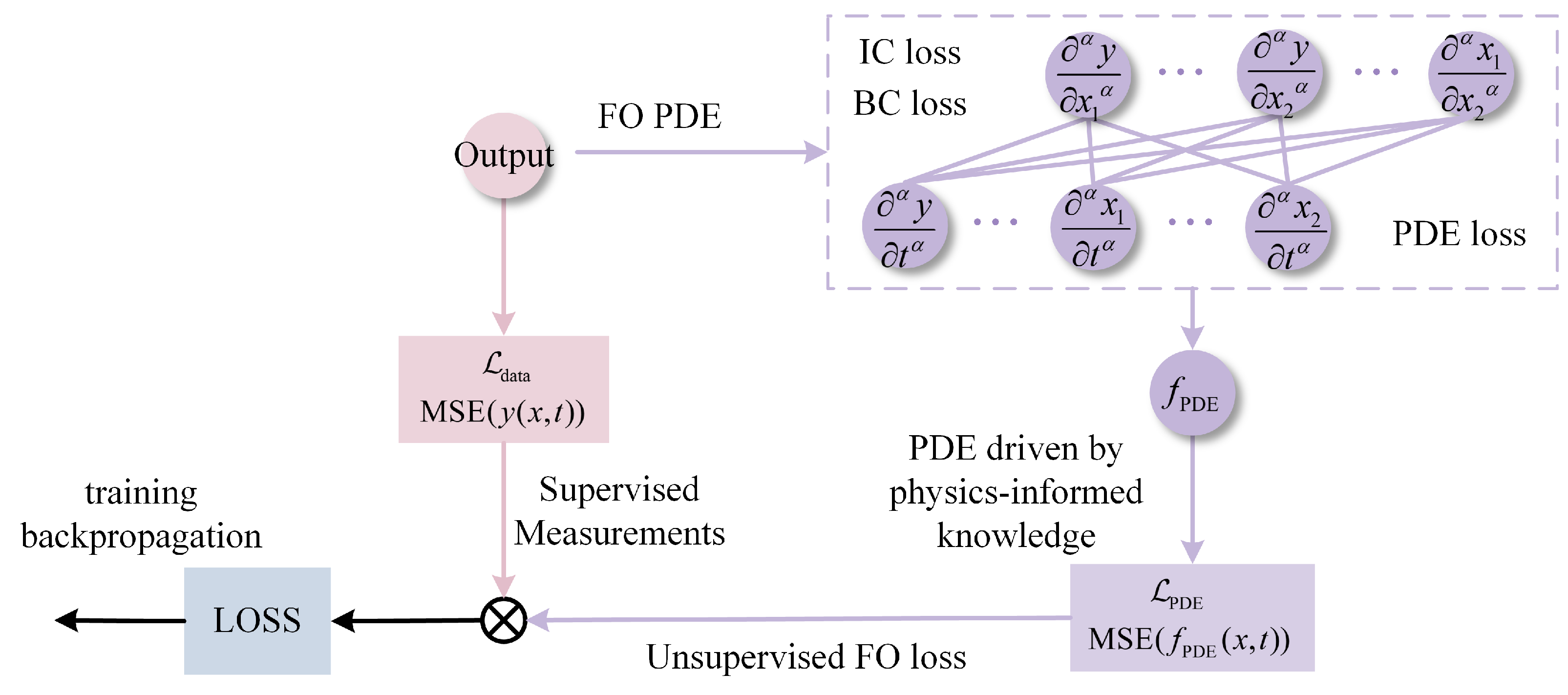
As provided in the introduction Section 1, the embedded physics information in ML algorithms were mainly concluded into observational bias, inductive bias, and learning bias [24]. A typical example of learning bias is that physics are enforced via soft penalty constraints into the loss function of NNs. In this subsection, the soft penalty constraint is realized by a fractional-order PDE reflecting battery knowledge and embedded into the loss function of RNN, as shown in Figure 4. Except for the common loss of the supervised measurement of outputs, a fractional-order PDE driven by physics-informed knowledge is added as an unsupervised fractional-order loss, constructing the final loss for training backpropagation.

3.2.1. Constraint in Fractional-Order PDE Form

As shown in Figure 4, the unsupervised constraint is in a fractional-order PDE form, which can include various types of fractional-order derivatives, such as PDE loss, initial condition (IC) loss, and boundary condition (BC) loss. The fractional-order PDE constraint is firstly presented in this part, then the specific fractional-order PDE for LIB is presented in the following part. The general form of a PDE with initial condition and boundary condition is given in Definition 3.
Definition 3.
PDE with initial and boundary conditions [36].
L [ y ] ( x ) = f ( x ) , x Ω × [ 0 , T ] , B [ y ] ( x ) = y b ( x ) , x Ω × [ 0 , T ] , y ( x , 0 ) = y 0 ( x ) , x Ω ,
where L and B represents the differential operators, Ω is the spatio-temporal domain, y is the solution, y b and y 0 are the boundary and initial functions.
The exact solution y * of the PDE in Definition 3 usually lies in an infinite dimensional space, and the FORNN with PDE constraint in this work would parameterize the solution y * of as y (18) to approximate the ground truth in a numerical way. If the differential operator in Definition 3 is chosen as integer-order derivative, it can obtain an integer-order PDE constraint as stated in Lemma 4.
Lemma 4.
If the differential operators in (18) is an integer-order derivative, a simple physics-informed PDE constraint can be presented as
f PDE ( x , t ) = y t + a 1 y x + a 2 2 y x 2 ,
where a 1 and a 2 are the coefficients of boundary condition loss (BC loss) and initial condition loss (IC loss). The PDE constraint in (19) satisfies a certain physics-informed law of the object, and (19) can be extended to a complex form with extra information by adding other types of derivatives more than IC loss or BC loss.
Remark 1.
The PDE constraint in Lemma 4 could be integer-order PDEs, integro-differential equations, fractional-order PDEs, or stochastic PDEs [24].
As stated in Remark 1, the PDE constraint in Lemma 4 may vary from different physical equations according to the investigated object in different problems, such as the viscous Burgers’ equation y t + y y x = v 2 y x 2 with a initial condition and Dirichlet boundary conditions. Considering the embedding battery knowledge represented by FOMs in this work, the integer-order PDE constraint in Lemma 4 would be extended to a fractional-order one, as stated in Lemma 5.
Lemma 5.
Combining with the various forms of fractional-order derivatives in Figure 4, and if the differential operators in (18) is a fractional-order derivative, the fractional-order PDE constraint with physics-informed knowledge can be presented as
f FOPDE ( x , t ) = α y t α PDE loss + a 1 α y x 1 α + a 2 α y x 2 α condition loss + b 1 α x 1 t α + b 2 α x 2 t α input constraint + c 1 α x 1 x 2 α coupled rate ,
where a i , i = 1 , 2 , b i , i = 1 , 2 , and c 1 are the coefficients of condition loss (such as IC loss and BC loss), input constraint, and coupled rate, respectively. The fractional-order PDE constraint f FOPDE ( x , t ) in (20) normalizes the coefficient of PDE loss ( α y / t α ) as 1, and sets the fractional order α as the same, which can be various in application. The fractional-order PDE constraint f FOPDE ( x , t ) in (20) satisfies a certain fractional-order physics-informed law of the object.
The fractional-order PDE constraint in Lemma 5 contains PDE loss, condition loss, input constraint, and coupled constraint. Among the four parts, input constraint may be the input derivative in time series, and coupled constraint may be the coupled rate or coupled relationships among inputs, which usually exists in physical systems. Note that the fractional-order PDE in (20) covers the integer-order one in (19) when the fractional-order is set as 1.
Lemma 6.
According to [24], and referring to the fractional-order PDE constraint in (20), the final loss function can be deduced as
L = w data L data + w PDE L PDE ,
where
L data = 1 N data i = 1 N data ( y ( x i , t i ) y i ) 2
is the supervised loss of data output error, and
L PDE = 1 N PDE j = 1 N PDE [ f FOPDE ( x , t ) ] 2 | ( x j , t j ) = 1 N PDE j = 1 N PDE ( α y t α + a i α y x m α + b i α x m t α + c i α x m x n α ) 2 | ( x j , t j , m = 1 , 2 , m n , n = 1 , 2 )
is the unsupervised loss of fractional-order PDE constraint f FOPDE ( x , t ) .
In (21)–(23), w data and w PDE are the weights to balance the two loss L data and L PDE ; y i are values of y at ( x i , t i ) ; ( x i , t i ) and ( x j , t j ) are two sets of points sampled at the initial/boundary locations and in the entire domain, respectively.
With Lemmas 5 and 6, the general form of a fractional-order PDE constraint is proposed to encode physics-informed knowledge into the loss function of FORNN. For a specific object, the physics-informed PDE in (20) should be extracted from certain equations by object modeling.

3.2.2. Constraint of Battery Terminal Voltage Derivative Equation

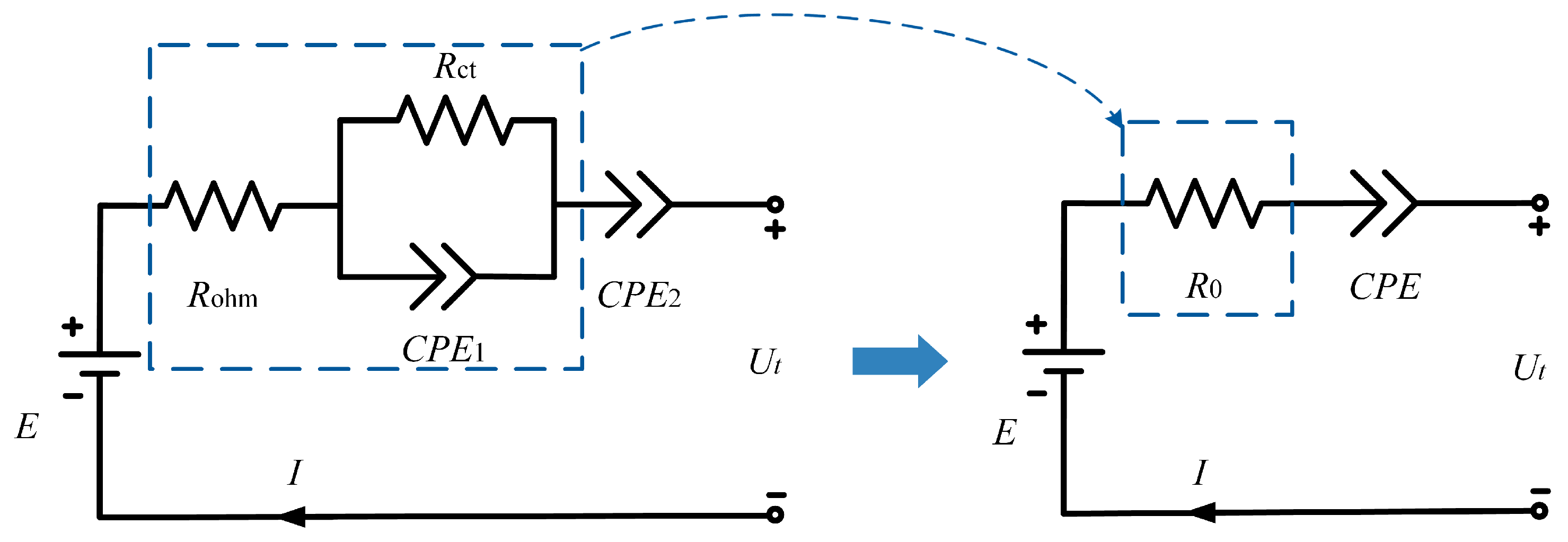
As introducing in Section 2.2, the physics-informed laws of LIBs can be described by fractional-order elements in battery FOM, which is a suitable choice to be transferred to the fractional-order PDE constraint as stated in Lemma 5. A second-order FOM is firstly considered in this work as shown in Figure 5 [37,38].
In Figure 5, the impedance of the second-order FOM in the left side can be presented as
Z = R ohm + Z ARC + Z Warburg = R ohm + R c t R c t C 1 s α 1 + 1 + 1 C 2 s α 2
where E is the open circuit voltage (OCV), U t is the terminal voltage, and R ohm , RC tank Z ARC ( R c t and C P E 1 ), and Z Warburg ( C P E 2 ) represent the ohmic resistance in high-frequency, double layer effects and charge transfer reactions in mid-frequency, and solid diffusion dynamics in low-frequency of EIS of LIBs, respectively. Specifically, the time constant of R ohm and RC tank Z ARC is less than 0.05 s and Z Warburg is longer than 50 s in the time scale [37], while the sampling frequency of general BMS is about 1 10 Hz, which cannot accurately identify the transient response of R ohm and the dynamic response of Z ARC . Considering R ohm and RC tank Z ARC as one process, the second-order FOM is simplified as a RC tank as shown in the right side of Figure 5, which has the impedance as
U t ( s ) E ( s ) I ( s ) = R 0 + Z Warburg = R 0 + 1 C s α ,
where R 0 = R ohm + Z ARC . Equation (25) acts as the basis of the fractional-order constraints for the loss function of PIRNN, which is furtherly deduced in the latter part.
Take the simplified FOM in Figure 5, and the corresponding voltage-current equation (25) can be presented as
U t ( s ) E ( s ) = ( R 0 + 1 C s α ) I ( s ) C s α ( U t ( s ) E ( s ) ) = ( R 0 C s α + 1 ) I ( s ) ,
where U t is the terminal voltage, E is the OCV, and I is the current; R 0 and C are the resistance part and capacity value of the FOM in Figure 5, respectively.
Applying inverse Laplace transform, transfer (26) into time domain as
C · D α ( u t ( t ) E ( t ) ) = ( R 0 C · D α + 1 ) i ( t ) ,
where u t ( t ) , E ( t ) , and i ( t ) are the time-series terminal voltage, OCV, and current in time domain. Rewrite (27) as
C α u t ( t ) t α = C α E ( t ) t α + R 0 C α i ( t ) t α + i ( t ) ,
In (28), the terminal voltage u t ( t ) and current i ( t ) can be directly obtained from realistic sampled EV data, while OCV E ( t ) is an inside variable of the battery that can be hardly measured in real operation conditions. However, SOC have a relationship with OCV, which can be approximately calculated as [39]
E ( t ) = f ( S O C ) = k = 0 d k S O C k ( t ) ,
where d k is the coefficients of S O C k ( t ) . Considering (28) as the fractional-order PDE constraint and a finite terms k in (29), some certain assumptions are proposed to replace OCV in (28) by SOC, as stated in Lemma 6.
Lemma 7.
According to the measured SOC-OCV curves in literature, let k in (29) holds k = 1 and assume OCV E ( t ) is monotonic with S O C ( t ) , so that the fractional-order derivative of E ( t ) holds the relationship with the fractional-order derivative of S O C ( t ) as
α E ( t ) t α = d s o c α S O C ( t ) t α ,
where d s o c is the ratio of ( α E ( t ) / t α ) to ( α S O C ( t ) / t α ) .
Take (30) into (28), we obtain the fractional-order PDE constraint from the FOM of battery as
C α u t ( t ) t α = d s o c C α S O C ( t ) t α + R 0 C α i ( t ) t α + i ( t ) .
For FORNN with PIBatKnow, the inputs and outputs should be carefully selected and combined with the fractional-order constraint (31). Moreover, it should consider the available variables from realistic data, the influence of temperature, and the aim of the proposed FORNN. For example, taking state estimation as target, then the inputs are defined as x ( t ) = [ x 1 ( t ) , x 2 ( t ) , x 3 ( t ) ] T = [ u t ( t ) , i ( t ) , T t e m p ( t ) ] T , and the output as y ( t ) = S O C ( t ) , thus the fractional-order PDE constraint can be deduced as
f S O C ( x , t ) = d s o c C α y ( t ) t α + R 0 C α x 2 ( t ) t α + x 2 ( t ) C α x 1 ( t ) t α ,
Combining (32) with (23), the loss of fractional-order PDE constraint can be calculated in the form of a mean sum of square (MSS), and embedded into the loss function as a fractional-order unsupervised loss. G-L definition can be employed to discrete the fractional-order derivatives in (32) for calculation. Select finite terms L = 5 in (2), and the fractional-order derivatives of inputs x ( t ) and output y ( t ) in (32) can be deduced as
Δ α M ( t ) = j = 0 5 ( 1 ) j α j M ( k j ) ,
where M ( t ) = x 1 ( t ) , x 2 ( t ) , or y ( t ) , and k is the discrete step. Note that the discrete equation in (33) requires the history data in previous { 5 j , ( j = 0 , 1 , , 5 ) } moments, which can be found in the time-series data of the realistic sampled voltage, current, and the output SOC. With (32) and (33), a FORNN with a fractional-order PDE constraint is constructed and encoded by battery voltage equation, then the proposed FORNN can be applied to conduct SOC estimation or further life prediction.

3.3. Fractional-Order Descent Methods

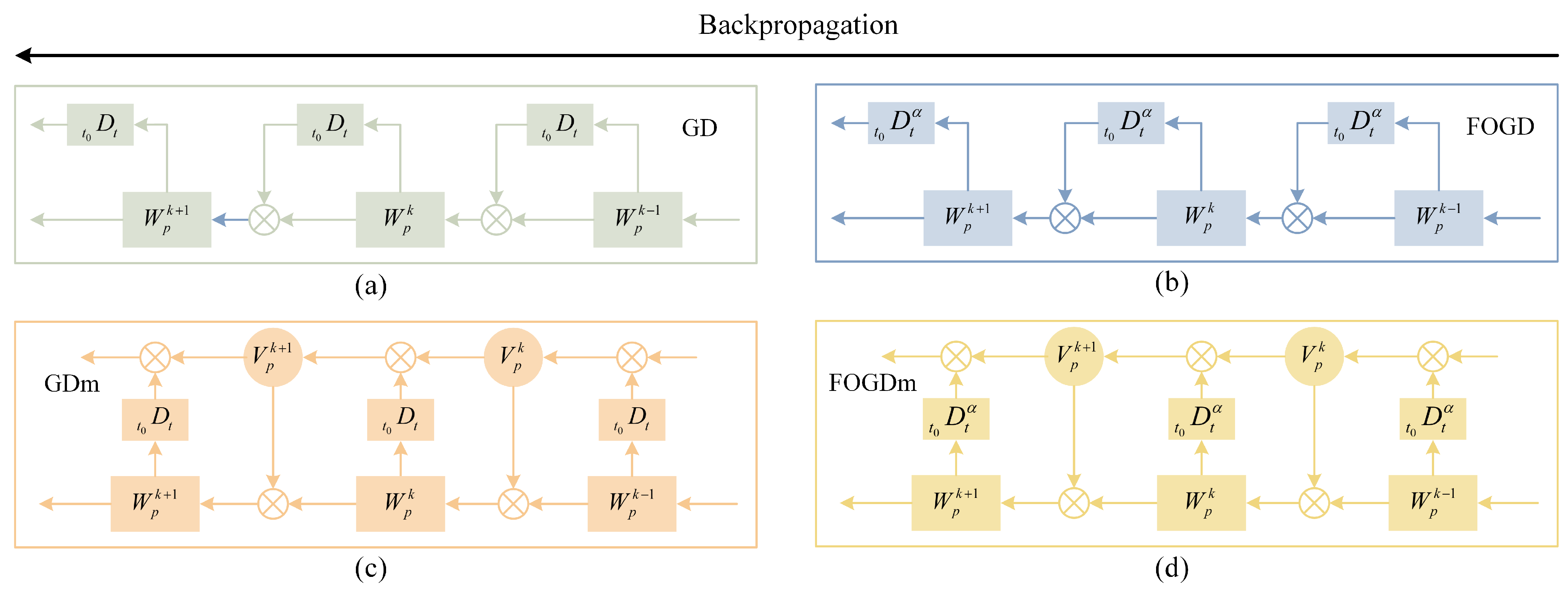
Besides fractional-order state feedback and fractional-order constraint, the FORNN can also be enhanced in the backpropagation process by fractional-order gradients. In the opposite direction of forward propagation, backpropagation starts from the output layer to the input layer, mainly updating weights W p , W h p , and bias b p , ( p = 1 , 2 , , l ) in the gradient descent direction, which is called the gradient descent (GD) method, as shown in Figure 6a. It always makes the weights W p = W h p in a realistic application, and the bias b p holds the same update with weight W p , thus only weight W p is discussed in the following. During backpropagation, the layer state gradients are calculated, then weight gradients are based on the layer gradients to update weight W p . The gradients of the p th hidden layer for the k th , ( k = 1 , 2 , , N ) input sample are presented as
L ( g ( x ) , y ) h p k ( x ) = W p + 1 k L ( g ( x ) , y ) a p + 1 k ( x ) L ( g ( x ) , y ) a p k ( x ) = L ( g ( x ) , y ) h p k ( x ) · g ( a p k ( x ) ) = W p + 1 k L ( g ( x ) , y ) a p + 1 k ( x ) · g ( a p k ( x ) ) ,
where L ( g ( x ) , y ) / h p k ( x ) and L ( g ( x ) , y ) / a p k ( x ) are the gradients of the output h p k ( x ) and the input a p k ( x ) of the p th hidden layer, respectively. Since the backpropagation starts from the output layer, it supposes that the gradients L ( g ( x ) , y ) / h t k ( x ) and L ( g ( x ) , y ) / a t k ( x ) of the t th , ( t = p + 1 , p + 2 , , l , l + 1 ) layer are already known. With layer gradients in (34), fractional-order derivative is introduced from the output layer to calculate the fractional-order gradients of loss function L ( g ( x ) , y ) ; then, all the weights gradients of hidden layers are transferred to fractional-order ones, which turns out to be a fractional-order gradient descent (FOGD) method, as shown in Figure 6b. For time-series battery dataset as the inputs of the proposed FORNN, if considering the gradient descent method with momentum (GDm) shown in Figure 6c, the FOGD method can be extended to the FOGD method with momentum (FOGDm), as presented in Figure 6d.

3.3.1. Fractional-Order Gradient Descent

FOGD employs the fractional-order gradients of the loss function and weights W p instead of the integer-order gradients. Based on the fractional-order gradient in (9), the FOGD for the updates of weight W p is presented as
W p k + 1 = W p k η · W p 0 D W p k α L ( f ( x ) , y ) = W p k η · α L ( f ( x ) , y ) W p k α
According to a p ( x ) = W p h p 1 ( x ) + b p in (12) and the chain rule, (35) is deduced as
W p k + 1 = W p k η · L ( g ( x ) , y ) a p k ( x ) · α a p k ( x ) W p k α
where L ( g ( x ) , y ) / ( W p k ) α is the fractional-order gradients of weight W p to the loss function L ( g ( x ) , y ) , and η is the learning rate (iteration step size). It should be noted that, according to Lemma 3 in Section 2.1.1, the chain rule in (36) for fractional-order partial derivatives only validates when the loss function L ( g ( x ) , y ) holds an exponential form as the function f ( x ) in (5). In (36), the gradient of the input a p k ( x ) to the loss function ( L ( g ( x ) , y ) / a p k ( x ) ) can be obtained by (34), and α a p k ( x ) / ( W p k ) α can be calculated by (5). Hence, combining (34) and the discrete Caputo definition in (5), the fractional-order gradients of weight W p to the loss function L ( g ( x ) , y ) can be deduced as
α L ( g ( x ) , y ) ( W p k ) α = h p 1 k ( x ) Γ ( 2 α ) · L ( g ( x ) , y ) a p k ( x ) W p k W p 0 1 α
where W p 0 is the initial values of weight W p . Take (37) into (36), we can obtain the FOGD method for backpropagation as
W p k + 1 = W p k η · h p 1 k ( x ) Γ ( 2 α ) · L ( f ( x ) , y ) a p k ( x ) W p k W p 0 1 α
where α is a fractional order that may be related to battery knowledge and sensitive to the training results. The sensitivity of the fractional order α and the corresponding influence on network output is discussed in the experimental part.

3.3.2. Fractional-Order Gradient Descent with Momentum

FOGDm method is extended from FOGD method by adding momentum, which demonstrates the changing direction of the fractional-order gradients. Given the integer-order gradient descent (GD) method with momentum as
V p k + 1 = μ · V p k η · L ( g ( x ) , y ) W p k W p k + 1 = W p k + V p k + 1
where μ is the momentum factor, which is the proportion of history gradient data, and V p is the weight momentum. Then the weight update by FOGDm method can be presented as
V p k + 1 = μ · V p k η · α L ( g ( x ) , y ) W p k α W p k + 1 = W p k + V p k + 1
Take the fractional-order gradients of weight W p to the loss function L ( g ( x ) , y ) in (37) into (40), we obtain the discrete updating equation of weight W p by the FOGDm method as
V p k + 1 = μ · V p k η · h p 1 k ( x ) Γ ( 2 α ) · L ( g ( x ) , y ) a p k ( x ) W p k W p 0 1 α W p k + 1 = W p k + V p k + 1
With (41) to encode the momentum of fractional-order gradient into the backpropagation process, the FOGDm method accelerates the convergence of the proposed FORNN with faster updates of weight W p and bias b p , and adjusts fractional-order gradients more rapidly than the FOGD method.

4. Experiment Setups

4.1. Battery and Operation Conditions

The proposed FORNN with PIBatKnow in this work may contain fractional-order state feedback, fractional-order loss constraint, and fractional-order gradient for backpropagation, which bring more parameters for algorithm tuning. Hence, the sensitivity analysis is necessary to identify suitable values and maximize the effectiveness for the practical estimation of LIB. For sensitivity analysis, experiments under five temperatures (5 C , 15 C , 25 C , 35 C , 45 C ) are conducted for a 18650 cell to collect battery data, and FUDS operation condition is employed to simulate the dynamic working condition. The parameters of the 18650 cell is shown in Table 1. The experimental data is sampled by a BTS-4 battery tester, and the cell is put in an incubator to control the testing temperature. The cell is fully charged by constant-current constant-voltage (CC-CV) method before applying FUDS, then fully discharged to the cut-off voltage 2.75 V under cycling FUDS periods.

4.2. Dataset and Initialization

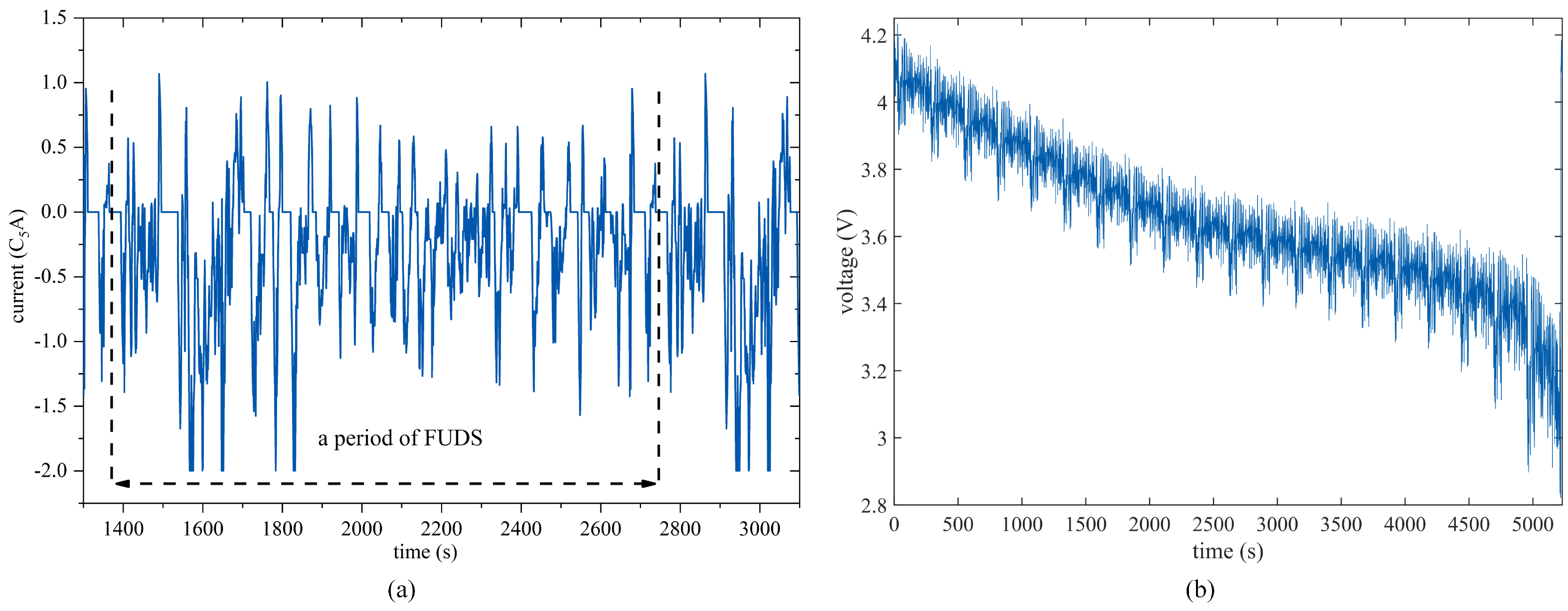
With the collected data, SOC is set as the estimation target of the proposed FORNN with PIBatKnow, so that the relationship between the input and the output can be constructed and analyzed clearly. The real SOC values are calculated by the ampere-hour integral method. Take the influence of temperature into consideration, this work for the sensitivity analysis takes the current, voltage, and temperature as the three main dimensions related to SOC. Hence, the inputs are selected as x ( t ) = [ x 1 ( t ) , x 2 ( t ) , x 3 ( t ) ] T = [ u t ( t ) , i ( t ) , T t e m p ( t ) ] T , and the output as y ( t ) = S O C ( t ) . Figure 7 is the current and voltage data after preprocess. The total amount of data is 27,213 points, which can support the big-data learning during training process for the proposed algorithm. The collected data is divided according to the five temperatures, that is, 45 C is selected as the testing data, and data under 5 C , 15 C , 25 C , and 35 C is divided into training data and validation data. The division ratio is 0.75:0.048:0.202, resulting in training data (20,410 points), validation data (1306 points), and testing data (5497 points). Since the aim of this work is the sensitivity analysis of parameters, only the data of one cell is enough, and any one of five temperatures (not specific 45 C ) can be selected as testing data. Moreover, some unchanged parameters are initialized and listed in Table 2.

5. Sensitivity Analysis and Estimation Results

After the dataset division and initialization of the proposed algorithm, the sensitivity of the main parameters related to the fractional-order knowledge are investigated in this work. According to Section 3, nine fractional-order parameters are investigated and divided into three categories, as shown in Table 3, that is, parameters’ sensitivity in the FOGD and FOGDm method (fractional-order gradient sensitivity), parameters’ sensitivity in fractional-order PDE constraint (impedance sensitivity), and weights in loss calculation (loss weight sensitivity). A certain possible range of the parameters are also provided in Table 3, in which only capacitance C bat and ohm resistance R 0 have physic units, that is, C and Ω , respectively, and other seven fractional-order parameters hold the unit 1. For example, the parameter range in impedance sensitivity is determined according to the battery FOM in (25) and Figure 5. With the three categories in Table 3 and other initialized network parameters in Table 2, the sensitivity analysis is conducted in the following sections, respectively.

5.1. Estimation with Fractional-Order Gradient Sensitivity

The first sensitivity category is the fractional-order gradient sensitivity, which contains the fractional order α 1 , the momentum weight μ , and the learning rate η in the FOGD and FOGDm method. Fractional order reflects and embeds battery fractional-order characteristics. In this section, only fractional order α 1 , momentum weight μ , and learning rate η change in the range provided in Table 3, respectively. Other parameters stay unchanged as shown in Table 4, and the default values of fractional order α 1 , momentum weight μ , and learning rate η are also provided when acting as the unchanged values in the other two sensitivity categories.
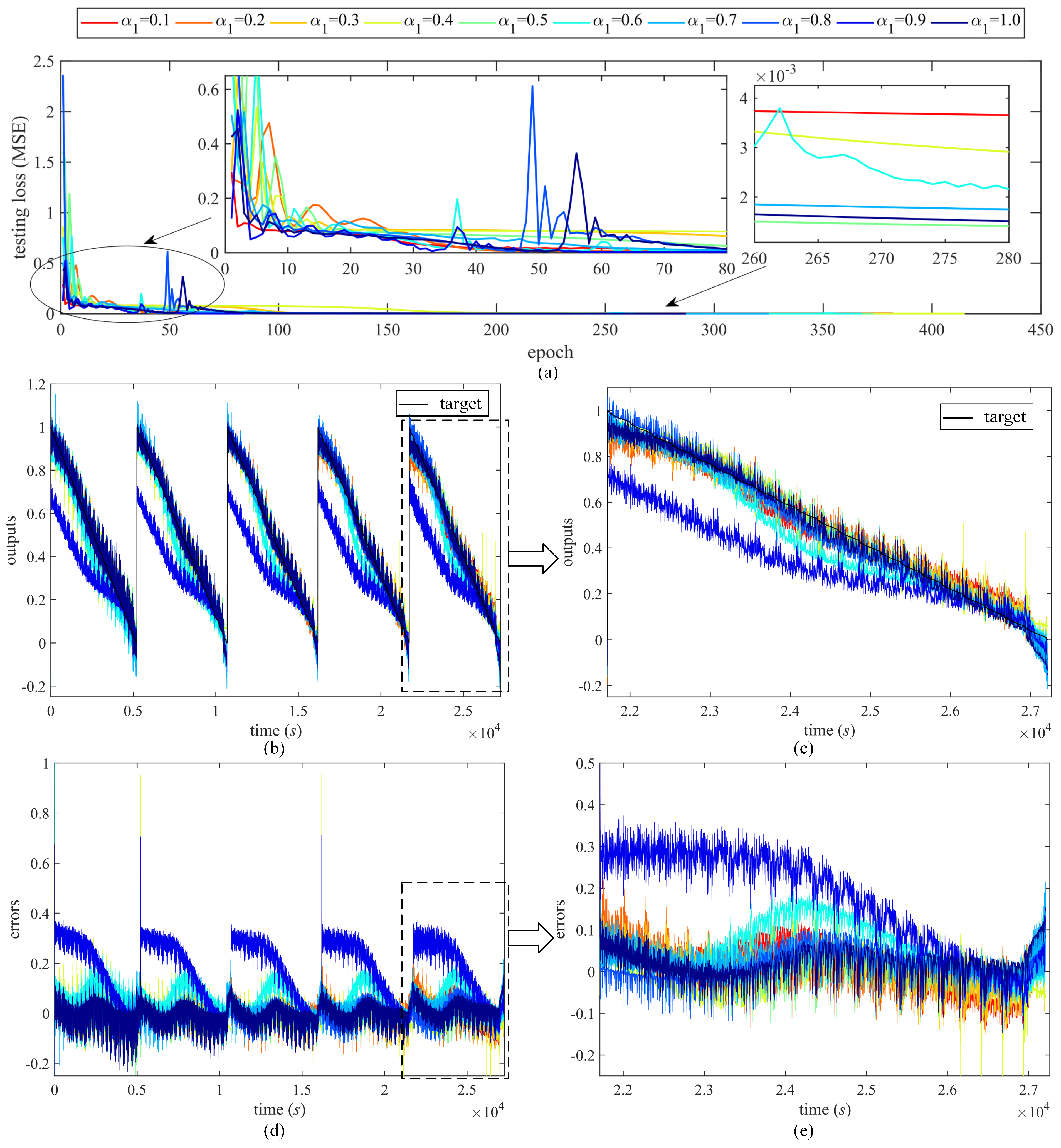
To verify the estimation effects, SOC is taken as the output of the proposed FORNN with PIBatKnow. Figure 8 presents the SOC estimation results under the sensitivity of the fractional order α 1 ( α 1 = 0.1:0.1:1) in FOGD and FOGDm methods. Expression variable = a:interval:b denotes that v a r i a b l e changes from a to b in the range [ a , b ] and takes the values in every interval i n t e r v a l , then this expression is applied to all the parameter sensitivity in the following part. Combined with Section 4.2, Figure 8b contains five discharging snippets under FUDS condition in five temperature (5 C , 15 C , 25 C , 35 C , 45 C ). Snippet in 45 C is the testing dataset, whose outputs and errors are enlarged in Figure 8c and Figure 8e, respectively.
The testing loss in Figure 8a shows that loss decreases and converges faster with larger α 1 , but the training process turns unstable when α > 0.5 , especially α = 1 . Moreover, the outputs of all dataset (training, validation, and testing) and errors (errors = target − outputs) are presented in Figure 8b and Figure 8d, respectively. Figure 8b,d also show the unstable accuracy performance. For fractional order α 1 , there exists a trade-off between performance and stability. With the outputs and the corresponding errors, it proves that the training dataset and testing dataset have similar performance, and the network does not overfit or underfit.
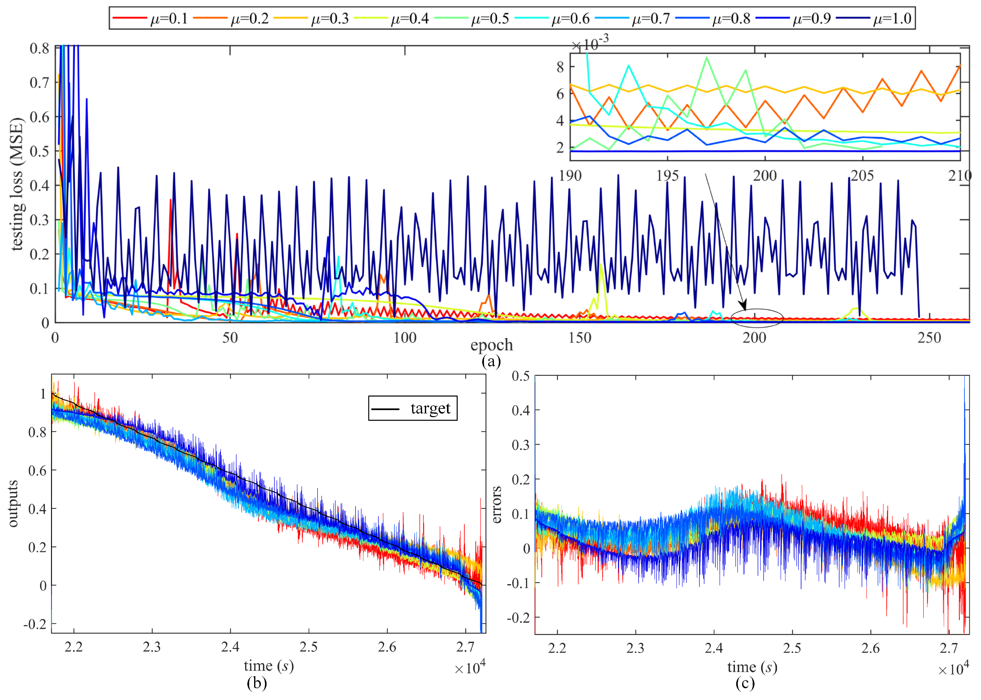
Similarly, the sensitivity of momentum μ and learning rate η are provided in Figure 9 and Figure 10, respectively. Since the testing prediction is the main point, and performance of the training or validation datasets are consistent with the testing dataset, only the testing outputs and testing errors are provided to focus on the testing performance, which is different from Figure 8.
From Figure 9, larger momentum weight μ would cause lower convergence speed and more instability, especially when μ = 1.0 , in which the network cannot converge, but the accuracy is enhanced by a larger μ . It should be noted that only the FOGDm method has the momentum weight μ , which determines the ratio of the previous momentum V p , as shown in (40). As to the learning rate η in Figure 10, it is very sensitive to the convergence speed and algorithm stability but not so sensitive to the accuracy, because the testing loss in Figure 10a varies a lot with different η , while the outputs and errors in Figure 10b,c do not show too much difference. A value of η larger than 0.2 is not suitable for the proposed FORNN with PIBatKnow.

5.2. Estimation with Impedance Sensitivity

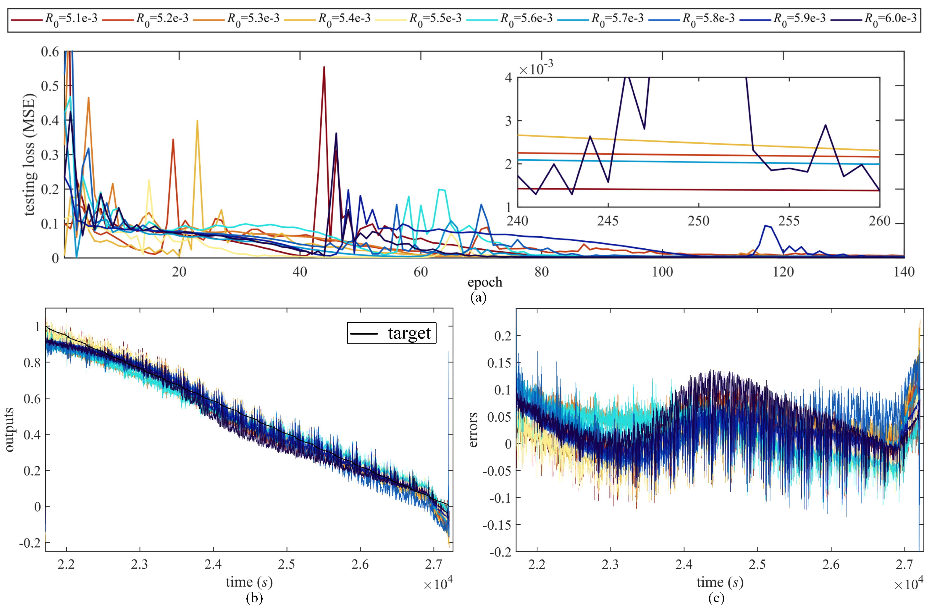
The second sensitivity category is the impedance sensitivity. For the fractional-order PDE constraint in loss function of the proposed FORNN with PIBatKnow, the main parameters include α 2 , d s o c , C bat , and R 0 of the battery FOM, and the sensitivity of the four impedance parameters are investigated in this section.
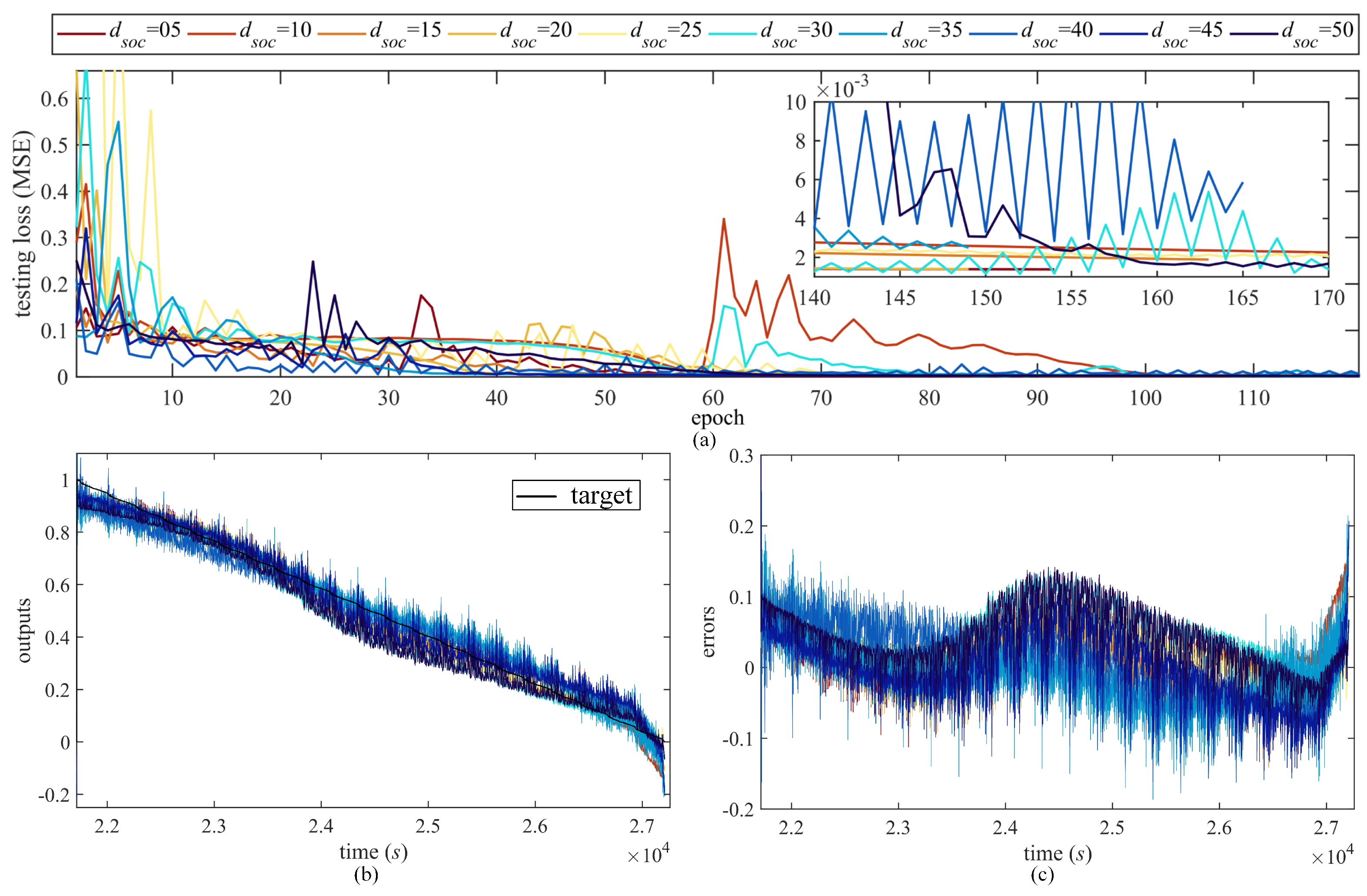
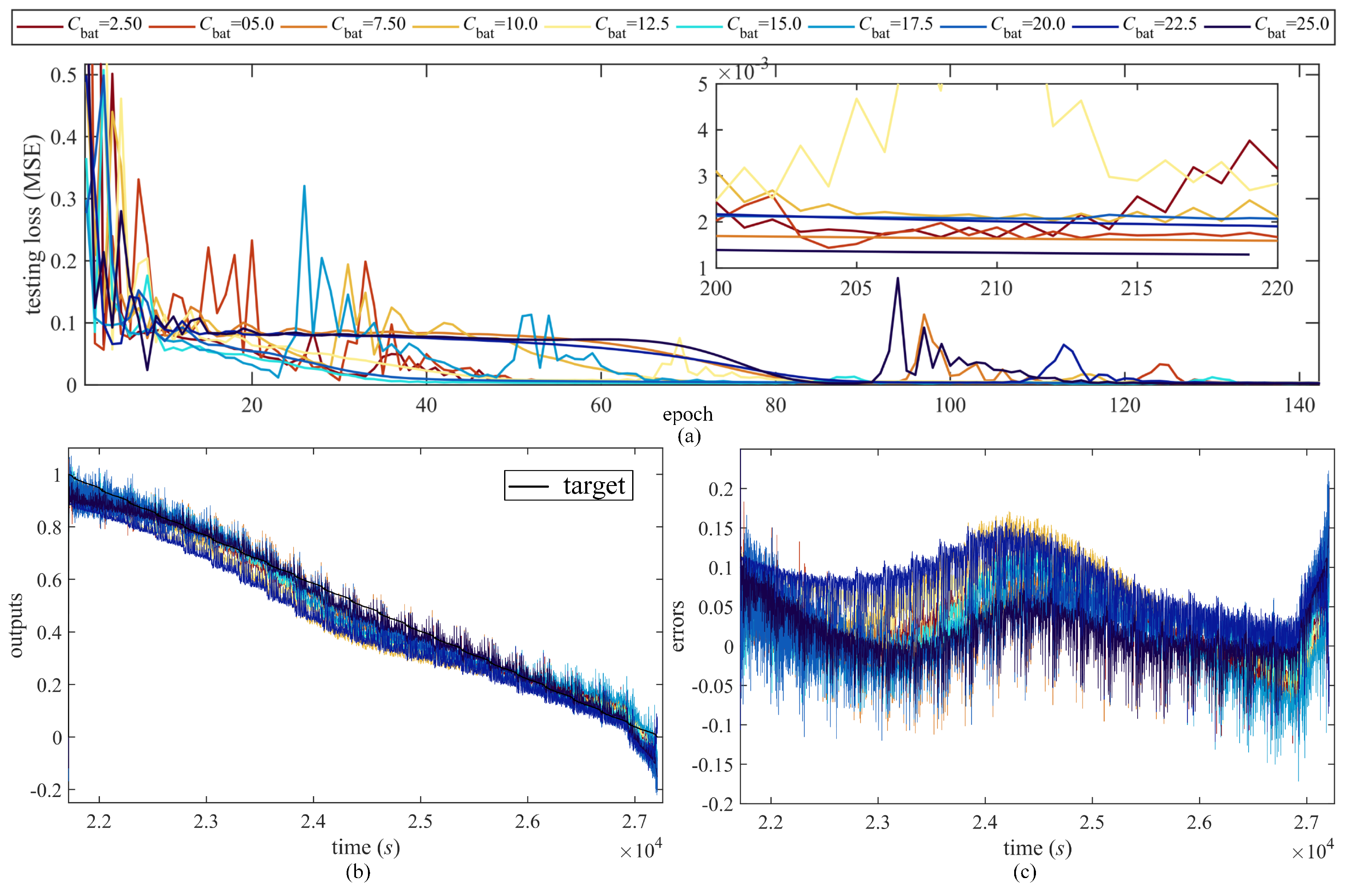
Figure 11, Figure 12, Figure 13 and Figure 14 are the testing loss, testing outputs, and corresponding errors under the four impedance parameters α 2 , d s o c , C bat , and R 0 , respectively. To better illustrate the loss value, the testing loss is enlarged within the early stage of epochs, and a subfigure enlarging the stable loss in later epochs is added in every figure of testing loss, like Figure 11a. Part of the training process would be terminated before the max epoch (300) when reaching the training goal (1.6 × 10 4 ) or other validation conditions. For example, in the subfigure of Figure 11a, the training process with α 2 = 0.1 stopped at 159th epoch. From the accuracy aspect, the outputs and errors in Figure 11, Figure 12, Figure 13 and Figure 14 do not show large fluctuations when the impedance parameters change. Most of the errors with various α 2 , d s o c , C bat , and R 0 maintain the magnitude within 0.15 .
From Figure 11, the testing loss decreases and becomes more stable with larger fractional order α 2 , and the errors also decrease to within 0.05 , as shown in Figure 11c. From Figure 12, the testing loss and outputs accuracy do not show certain sensitive pattern when the ratio d s o c between OCV and SOC changes, but the testing loss becomes more unstable with larger d s o c . From Figure 13, the testing loss converges faster when the capacitance C bat is in the middle value (such as 15 , 17.5 , 20 ). The stable loss becomes flatter and the errors become smaller with larger C bat . From Figure 14, a large resistance R 0 would cause unstable convergence process and large testing loss, but the estimation accuracy in high SOC range may be improved.

5.3. Estimation with Loss Weight Sensitivity

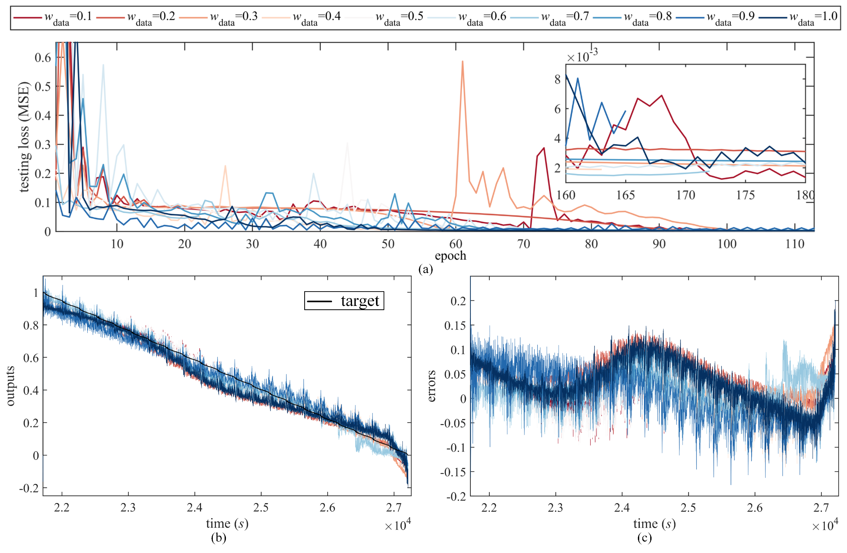
The third sensitivity category is the loss weight sensitivity. The loss weight w data and w PDE can determine the ratio of the supervised measurement loss and the unsupervised fractional-order loss calculated by physics-informed PDE in Figure 4. Since loss weight w data and w PDE hold the relationship w PDE = 1 w data , the two parameters may be considered as one parameter sensitivity, as presented in Figure 15. w data = 0.1:0.1:1 corresponds to w PDE = 0.9:0.1:0. The testing loss in Figure 15a demonstrates that larger w data makes the network process converge faster and more stable, which reflects the relative instability of the physics-informed knowledge embedding. However, the algorithm can achieve a trade-off with sensitivity analysis and suitable tuning. As to the estimation accuracy, the outputs and errors in Figure 15b,c do not show much improvement both in the small value and large value of w data .

5.4. Correlation Analysis

Correlation analysis is provided in this section to present the dynamic relationship between parameters and the proposed algorithm performance. Based on the possible range in Table 3, the three categories (nine parameters) are sampled as ten groups of values randomly, as shown in Table 5. Mean square error (MSE) is selected as the evaluation function in this work, thus the change of MSE is considered as the indicator of the algorithm performance, marked as p e r f and presented in Table 5. Despite the total MSE p e r f , the performance of training dataset, validation dataset, and testing dataset can be calculated as t r p e r f , v p e r f , and t p e r f , respectively.
To quantize the dynamic trend between the nine fractional-order parameters and algorithm performance, the Pearson correlation coefficients are calculated with Table 3 and listed in Table 6. From the correlation coefficients in Table 6, the fractional order α 1 in gradients and learning rate η have a strong influence on the algorithm, while the momentum weight μ in the gradient method mainly contributes to the validation performance. The impedance (mainly d s o c , C bat , and R 0 ) of battery FOM (25) have strong correlations with the validation performance and testing performance, while the fractional order α 2 has weaker influence on the testing dataset. The loss weight w data and w PDE have weaker influence on training performance than the other parameters, but the two of them have the same correlation coefficients due to the relationship w PDE = 1 w data . The total performance p e r f and training performance t r p e r f have very close values because the division ratio is 0.75:0.048:0.202, which demonstrates that training performance constructs the main part of the total performance.

6. Discussion

Combined with the estimation results under the three sensitivity categories and the correlation analysis, the sensitivity and correlation of the nine main fractional-order parameters to the algorithm performance can be concluded as shown in Table 7.
Take convergence speed, testing loss, estimation accuracy, and stability as the algorithm performance indexes, several notes can be listed as references and instructions for the tuning of the nine main fractional-order parameters in the proposed FORNN with PIBatKnow as follows.
  • For the convergence speed, it would be boosted by a larger value of α 1 , d s o c , and w data , and by a smaller value of μ , η , α 2 , R 0 , and w PDE ;
  • For the testing loss, it would be improved by a larger value of α 1 , μ , and α 2 , and by a smaller value of R 0 , but does not show sensitivity to η , d s o c , C bat , w PDE , and w data ;
  • For the estimation accuracy, it would be improved by a larger value of α 1 , μ , α 2 , C bat , and R 0 , but does not show sensitivity to η , d s o c , w PDE , and w data ;
  • For the algorithm stability, it would be enhanced by a larger value of α 2 , C bat , and w PDE , and by a smaller value of α 1 , μ , η , d s o c , R 0 and w PDE ;
  • According to the correlation analysis, if the nine fractional-order parameters can be tuned adaptively, the fractional order α 1 , the learning rate η , and the capacitance C bat have the most dynamic correlation to the performance;
  • For the fractional order α 1 in FOGD and FOGDm methods, a value in range ( 0.5 , 1 ) is suitable and a trade-off would be made between performance and stability;
  • The ratio of the previous momentum V p , larger μ means larger inertia of the previous convergence, which makes the speed slow but improves the learning ability to achieve higher accuracy;
  • The proposed algorithm achieves faster convergence speed in the middle values of the capacitance C bat in battery FOM;
  • The loss weight w PDE has opposite tuning direction to the loss weight w data .

7. Conclusions

This paper presents the sensitivity analysis of a fractional-order recurrent neural network (FORNN) with physics-informed knowledge of lithium-ion battery. A recurrent neural network is physics-informed by encoding with fractional-order battery knowledge, resulting in the proposed algorithm, called FORNN with PIBatKnow. Three types of physics-informed patterns are proposed as the fractional-order state feedback for forward propagation, the fractional-order PDE constraint for loss function, and the FOGD methods for backpropagation. Then, the sensitivity of nine main fractional-order parameters from the FOGD and FOGDm methods, the battery FOM, and the loss calculation are taken into consideration. Both SOC estimation experiment under parameter sensitivity and correlation analysis are conducted. Several notes and discussions are presented to provide possible instructions for the tuning of the fractional-order parameters in the proposed FORNN with PIBatKnow. The discretization of fractional-order derivatives is the key point to embed fractional-order dynamics into neural network. For example, the fractional-order state feedback can be achieved by changing the discrete state calculating equations of the hidden layer; the fractional-order constraints need to rewrite the loss function code with the GL discrete form; the FOGD methods need to rewrite the training function code to introduce fractional-order gradients in the discrete form. As presented in the theoretical section Section 3, the fractional-order state feedback, the fractional-order constraints, and the FOGD methods can also be applied to other objects more than batteries. It only needs to transfer the fractional-order constraints related to the fractional-order physics knowledge of the other objects, and all methods in this work can be easily employed.
In future research, an enhanced FORNN can be furtherly investigated by improving fractional-order dynamics of the RNN system. The Caputo and GL derivatives used in this work can partly capture the battery mechanism dynamics to achieve faster convergence speed or higher estimation accuracy, and further discussion about the employed fractional-order definitions in the FORNN can be conducted in our future work. Specifically, the fractional-order derivatives can be furtherly improved, such as employing the fractional-order Caputo-Fabrizio or Atangana-Baleanu-Caputo derivative instead of the Caputo and GL derivative, the explanations of fractional-order derivative in the FORNN, and so on. Moreover, the fractional-order neural network is the combination of battery fractional-order modeling with machine learning; thus, more fractional-order information may be added into the network design to develop a physics-informed system. Hence, the fractional-order neural network can be enhanced by designing a specialized architecture of RNN. For example, FORNN with physics embedded in the loss function can be extended into multi-task learning algorithms, by introducing a set of physical constraints from various LIBs.

Author Contributions

Conceptualization, Y.W. and Y.C.; methodology, Y.W. and Y.C.; software, Y.W.; validation, Y.W.; formal analysis, Y.W.; investigation, Y.W. and X.H.; resources, X.H.; data curation, X.H. and M.O.; writing—original draft preparation, Y.W.; writing—review and editing, X.H., L.L. and Y.C.; supervision, M.O.; project administration, X.H. and M.O.; funding acquisition, Y.W., X.H. and M.O. All authors have read and agreed to the published version of the manuscript.

Funding

This research was funded by National Natural Science Foundation of China under Grant No. 62103220 and No. 52177217, Beijing Natural Science Foundation under Grant No. 3212031.

Data Availability Statement

Not applicable.

Conflicts of Interest

The authors declare no conflict of interest.

Sample Availability

Not applicable.

References

  1. Yang, R.; Xiong, R.; Ma, S.; Lin, X. Characterization of external short circuit faults in electric vehicle Li-ion battery packs and prediction using artificial neural networks. Appl. Energy 2020, 260, 114253. [Google Scholar] [CrossRef]
  2. Roman, D.; Saxena, S.; Robu, V.; Pecht, M.; Flynn, D. Machine learning pipeline for battery state-of-health estimation. Nat. Mach. Intell. 2021, 3, 447–456. [Google Scholar] [CrossRef]
  3. Tanim, T.R.; Dufek, E.J.; Walker, L.K.; Ho, C.D.; Hendricks, C.E.; Christophersen, J.P. Advanced diagnostics to evaluate heterogeneity in lithium-ion battery modules. ETransportation 2020, 3, 100045. [Google Scholar] [CrossRef]
  4. Wang, Y.; Tian, J.; Sun, Z.; Wang, L.; Xu, R.; Li, M.; Chen, Z. A comprehensive review of battery modeling and state estimation approaches for advanced battery management systems. Renew. Sustain. Energy Rev. 2020, 131, 110015. [Google Scholar] [CrossRef]
  5. Lu, Y.; Li, K.; Han, X.; Feng, X.; Chu, Z.; Lu, L.; Huang, P.; Zhang, Z.; Zhang, Y.; Yin, F.; et al. A method of cell-to-cell variation evaluation for battery packs in electric vehicles with charging cloud data. ETransportation 2020, 6, 100077. [Google Scholar] [CrossRef]
  6. Schindler, M.; Sturm, J.; Ludwig, S.; Schmitt, J.; Jossen, A. Evolution of initial cell-to-cell variations during a three-year production cycle. ETransportation 2021, 8, 100102. [Google Scholar] [CrossRef]
  7. Su, L.; Wu, M.; Li, Z.; Zhang, J. Cycle life prediction of lithium-ion batteries based on data-driven methods. ETransportation 2021, 10, 100137. [Google Scholar] [CrossRef]
  8. Yang, H.; Wang, P.; An, Y.; Shi, C.; Sun, X.; Wang, K.; Zhang, X.; Wei, T.; Ma, Y. Remaining useful life prediction based on denoising technique and deep neural network for lithium-ion capacitors. ETransportation 2020, 5, 100078. [Google Scholar] [CrossRef]
  9. How, D.N.; Hannan, M.; Lipu, M.H.; Ker, P.J. State of charge estimation for lithium-ion batteries using model-based and data-driven methods: A review. IEEE Access 2019, 7, 136116–136136. [Google Scholar] [CrossRef]
  10. Lipu, M.H.; Hannan, M.; Hussain, A.; Ayob, A.; Saad, M.H.; Karim, T.F.; How, D.N. Data-driven state of charge estimation of lithium-ion batteries: Algorithms, implementation factors, limitations and future trends. J. Clean. Prod. 2020, 277, 124110. [Google Scholar] [CrossRef]
  11. Wang, Y.; Wang, L.; Li, M.; Chen, Z. A review of key issues for control and management in battery and ultra-capacitor hybrid energy storage systems. ETransportation 2020, 4, 100064. [Google Scholar] [CrossRef]
  12. Han, X.; Feng, X.; Ouyang, M.; Lu, L.; Li, J.; Zheng, Y.; Li, Z. A comparative study of charging voltage curve analysis and state of health estimation of lithium-ion batteries in electric vehicle. Automot. Innov. 2019, 2, 263–275. [Google Scholar] [CrossRef] [Green Version]
  13. Zhu, J.; Wang, Y.; Huang, Y.; Bhushan Gopaluni, R.; Cao, Y.; Heere, M.; Mühlbauer, M.J.; Mereacre, L.; Dai, H.; Liu, X.; et al. Data-driven capacity estimation of commercial lithium-ion batteries from voltage relaxation. Nat. Commun. 2022, 13, 2261. [Google Scholar] [CrossRef] [PubMed]
  14. Tian, J.; Xiong, R.; Yu, Q. Fractional-order model-based incremental capacity analysis for degradation state recognition of lithium-ion batteries. IEEE Trans. Ind. Electron. 2018, 66, 1576–1584. [Google Scholar] [CrossRef]
  15. Li, S.; Hu, M.; Li, Y.; Gong, C. Fractional-order modeling and SOC estimation of lithium-ion battery considering capacity loss. Int. J. Energy Res. 2019, 43, 417–429. [Google Scholar] [CrossRef] [Green Version]
  16. Nasser-Eddine, A.; Huard, B.; Gabano, J.D.; Poinot, T. A two steps method for electrochemical impedance modeling using fractional order system in time and frequency domains. Control Eng. Pract. 2019, 86, 96–104. [Google Scholar] [CrossRef]
  17. Wang, X.; Wei, X.; Zhu, J.; Dai, H.; Zheng, Y.; Xu, X.; Chen, Q. A review of modeling, acquisition, and application of lithium-ion battery impedance for onboard battery management. ETransportation 2021, 7, 100093. [Google Scholar] [CrossRef]
  18. Sulzer, V.; Mohtat, P.; Aitio, A.; Lee, S.; Yeh, Y.T.; Steinbacher, F.; Khan, M.U.; Lee, J.W.; Siegel, J.B.; Stefanopoulou, A.G.; et al. The challenge and opportunity of battery lifetime prediction from field data. Joule 2021, 5, 1934–1955. [Google Scholar] [CrossRef]
  19. Feng, X.; Merla, Y.; Weng, C.; Ouyang, M.; He, X.; Liaw, B.Y.; Santhanagopalan, S.; Li, X.; Liu, P.; Lu, L.; et al. A reliable approach of differentiating discrete sampled-data for battery diagnosis. ETransportation 2020, 3, 100051. [Google Scholar] [CrossRef]
  20. Ng, M.F.; Zhao, J.; Yan, Q.; Conduit, G.J.; Seh, Z.W. Predicting the state of charge and health of batteries using data-driven machine learning. Nat. Mach. Intell. 2020, 2, 161–170. [Google Scholar] [CrossRef]
  21. Tian, J.; Xiong, R.; Shen, W.; Lu, J.; Yang, X.G. Deep neural network battery charging curve prediction using 30 points collected in 10 min. Joule 2021, 5, 1521–1534. [Google Scholar] [CrossRef]
  22. Hong, J.; Wang, Z.; Chen, W.; Wang, L.; Lin, P.; Qu, C. Online accurate state of health estimation for battery systems on real-world electric vehicles with variable driving conditions considered. J. Clean. Prod. 2021, 294, 125814. [Google Scholar] [CrossRef]
  23. Chen, Z.; Zhao, H.; Zhang, Y.; Shen, S.; Shen, J.; Liu, Y. State of health estimation for lithium-ion batteries based on temperature prediction and gated recurrent unit neural network. J. Power Source 2022, 521, 230892. [Google Scholar] [CrossRef]
  24. Karniadakis, G.E.; Kevrekidis, I.G.; Lu, L.; Perdikaris, P.; Wang, S.; Yang, L. Physics-informed machine learning. Nat. Rev. Phys. 2021, 3, 422–440. [Google Scholar] [CrossRef]
  25. Hu, T.; He, Z.; Zhang, X.; Zhong, S. Finite-time stability for fractional-order complex-valued neural networks with time delay. Appl. Math. Comput. 2020, 365, 124715. [Google Scholar] [CrossRef]
  26. Huang, Y.; Yuan, X.; Long, H.; Fan, X.; Cai, T. Multistability of fractional-order recurrent neural networks with discontinuous and nonmonotonic activation functions. IEEE Access 2019, 7, 116430–116437. [Google Scholar] [CrossRef]
  27. Lai, X.; Yi, W.; Cui, Y.; Qin, C.; Han, X.; Sun, T.; Zhou, L.; Zheng, Y. Capacity estimation of lithium-ion cells by combining model-based and data-driven methods based on a sequential extended Kalman filter. Energy 2021, 216, 119233. [Google Scholar] [CrossRef]
  28. Wang, Y.; Chen, Y.; Liao, X. State-of-art survey of fractional order modeling and estimation methods for lithium-ion batteries. Fract. Calc. Appl. Anal. 2019, 22, 1449–1479. [Google Scholar] [CrossRef]
  29. Alsaedi, A.; Ahmad, B.; Kirane, M. A survey of useful inequalities in fractional calculus. Fract. Calc. Appl. Anal. 2017, 20, 574–594. [Google Scholar] [CrossRef]
  30. Zhang, Q.; Shang, Y.; Li, Y.; Cui, N.; Duan, B.; Zhang, C. A novel fractional variable-order equivalent circuit model and parameter identification of electric vehicle Li-ion batteries. ISA Trans. 2020, 97, 448–457. [Google Scholar] [CrossRef]
  31. Marc, W. Efficient Numerical Methods for Fractional Differential Equations and Their Analytical Background. Ph.D. Thesis, Technischen Universität Braunschweig, Braunschweig, Germany, 2005. [Google Scholar]
  32. Lovoie, J.L.; Osler, T.; Tremblay, R. Fractional derivatives and special functions. SIAM Rev. 1976, 18, 240–268. [Google Scholar] [CrossRef]
  33. Khan, S.; Ahmad, J.; Naseem, I.; Moinuddin, M. A novel fractional gradient-based learning algorithm for recurrent neural networks. Circuits Syst. Signal Process. 2018, 37, 593–612. [Google Scholar] [CrossRef]
  34. Chen, Y.; Gao, Q.; Wei, Y.; Wang, Y. Study on fractional order gradient methods. Appl. Math. Comput. 2017, 314, 310–321. [Google Scholar] [CrossRef]
  35. Mu, H.; Xiong, R.; Zheng, H.; Chang, Y.; Chen, Z. A novel fractional order model based state-of-charge estimation method for lithium-ion battery. Appl. Energy 2017, 207, 384–393. [Google Scholar] [CrossRef]
  36. Peng, W.; Zhang, J.; Zhou, W.; Zhao, X.; Yao, W.; Chen, X. IDRLnet: A physics-informed neural network library. arXiv 2021, arXiv:2107.04320. [Google Scholar]
  37. Guo, D.; Yang, G.; Feng, X.; Han, X.; Lu, L.; Ouyang, M. Physics-based fractional-order model with simplified solid phase diffusion of lithium-ion battery. J. Energy Storage 2020, 30, 101404. [Google Scholar] [CrossRef]
  38. Guo, D.; Yang, G.; Han, X.; Feng, X.; Lu, L.; Ouyang, M. Parameter identification of fractional-order model with transfer learning for aging lithium-ion batteries. Int. J. Energy Res. 2021, 45, 12825–12837. [Google Scholar] [CrossRef]
  39. Zou, C.; Hu, X.; Dey, S.; Zhang, L.; Tang, X. Nonlinear fractional-order estimator with guaranteed robustness and stability for lithium-ion batteries. IEEE Trans. Ind. Electron. 2017, 65, 5951–5961. [Google Scholar] [CrossRef]
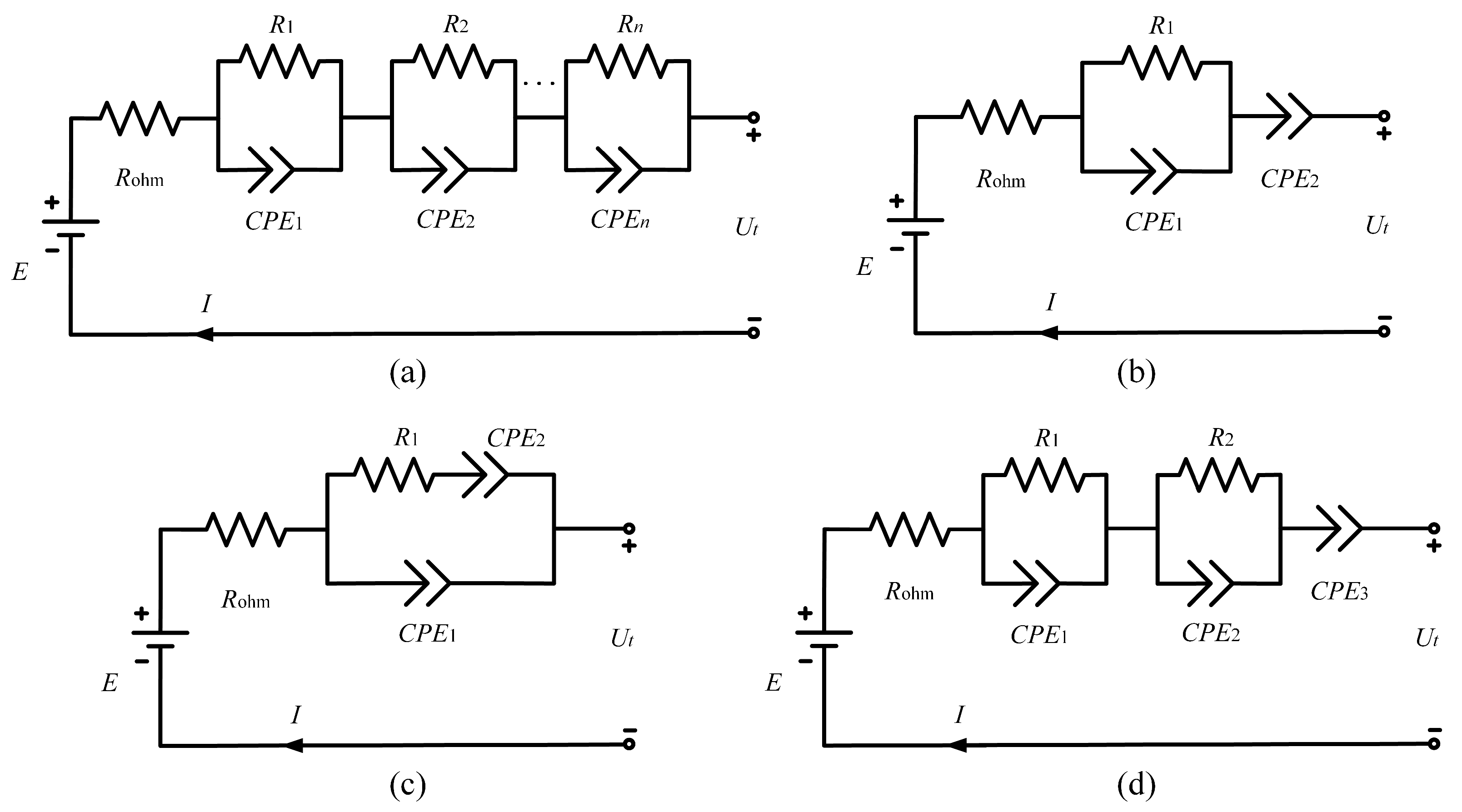
Figure 1. Fractional-order equivalent circuit model of LIBs in various forms, (a) n- R C α Model, (b) fractional-order PNGV model, (c) fractional-order Randles model, and (d) three-orders fractional-order model ( C P E i , i = 1 , 2 , , n ).
Fractalfract 06 00640 g001
Figure 2. Fractional-order recurrent neural network encoding with physics-informed battery knowledge.
Fractalfract 06 00640 g002
Figure 3. Fractional-order state feedback in the forward propagation of recurrent neural network, (a) integer-order state feedback, and (b) fractional-order state feedback.
Fractalfract 06 00640 g003
Figure 4. Fractional-order partial differential equation constraint.
Fractalfract 06 00640 g004
Figure 5. Simplifie FOM of LIBs as fractional-order PDE constraint.
Fractalfract 06 00640 g005
Figure 6. Fractional-order gradient descent methods, (a) integer-order GD method, (b) fractional-order GD method (FOGD), (c) integer-order GD method with momentum (GDm), and (d) fractional-order GD method with momentum (FOGDm).
Fractalfract 06 00640 g006
Figure 7. Collected dataset, (a) current in FUDS operation condition; (b) voltage in FUDS operation condition.
Fractalfract 06 00640 g007
Figure 8. Sensitivity of the fractional order α 1 in FOGD and FOGDm method, α 1 = 0.1:0.1:1, (a) testing loss, (b) outputs of all dataset including training, validation, and testing data, (c) outputs of testing dataset, (d) errors of all dataset, (e) errors of testing dataset.
Fractalfract 06 00640 g008
Figure 9. Sensitivity of the momentum of fractional-order gradient, μ = 0.1:0.1:1, (a) testing loss, (b) testing outputs, and (c) testing errors.
Fractalfract 06 00640 g009
Figure 10. Sensitivity of the learning rate, η = 0.08:0.02:0.26, (a) testing loss, (b) testing outputs, and (c) testing errors.
Fractalfract 06 00640 g010
Figure 11. Sensitivity of the fractional order α 2 in PDE constraint encoded into loss function, α 2 = 0.1:0.1:1, (a) testing loss, (b) testing outputs, and (c) testing errors.
Fractalfract 06 00640 g011
Figure 12. Sensitivity of the ratio d s o c between OCV and SOC in battery FOM for fractional-order PDE constraint, d s o c = 5:5:50, (a) testing loss, (b) testing outputs, and (c) testing errors.
Fractalfract 06 00640 g012
Figure 13. Sensitivity of the capacitance C bat in battery FOM for fractional-order PDE constraint, C bat = 2.5:2.5:25, (a) testing loss, (b) testing outputs, and (c) testing errors.
Fractalfract 06 00640 g013
Figure 14. Sensitivity of the ohm resistance R 0 in battery FOM for fractional-order PDE constraint, R 0 = 5.1 × 10 3 :1 × 10 4 :6 × 10 3 , (a) testing loss, (b) testing outputs, and (c) testing errors.
Fractalfract 06 00640 g014
Figure 15. Sensitivity of the loss weights w data and w PDE in loss function calculation, w data = 0.1:0.1:1, (a) testing loss, (b) testing outputs, and (c) testing errors.
Fractalfract 06 00640 g015
Table 1. LIB 18650 cell parameters.
ParametersValuesParametersValues
Rated capacity (0.5 C 5 A)2000 mAhRated voltage3.7 V
Max charge voltage4.2 VDischarge cut-off voltage2.75 V
Working temperature (charge)0 C –45 C Working temperature (discharge)−20 ° C –60 ° C
Table 2. Unchanged parameters of the proposed FORNN with PIBatKnow.
NameValue/RangeNameValue/Range
Hidden layers1Hidden neurons12
max epoch E max 300Performance functionMSE
train:valid:test0.75:0.048:0.202Training goal1.6 × 10 4
Table 3. Sensitivity categories of the fractional-order constraint and the fractional-order gradient in the proposed algorithm.
TypeNameValue/RangeAttribution
Fractional-order
Gradient sensitivity
Fractional order α 1 [ 0.1 , 1 ] FOGDm in (41)
Momentum weight μ [ 0.1 , 1 ]
Learning rate η [ 0.08 , 0.26 ]
Impedance sensitivityFractional order α 2 [ 0.1 , 1 ] FO PDE f S O C ( x , t ) in (32)
Ratio of OCV-SOC d s o c [ 5 , 50 ]
Capacitance C bat (unit: C) [ 2.5 , 25 ]
ohm resistance R 0 (unit: Ω )[5 × 10 3 , 6 × 10 3 ]
Loss weight sensitivityLoss weight w data [ 0.1 , 1 ] final loss L in (20)
Loss weight w PDE 1 w data
Table 4. Default values of the nine main fractional-order parameters.
α 1 μ η α 2 d soc C bat R 0 w data w PDE
0.90.750.180.940200.0050.80.2
Table 5. Ten groups of radom values of the nine parameters in the three categories for correlation analysis.
No. α 1 μ η α 2 d soc C bat R 0 w data w PDE perf trperf vperf tperf
110.720.1250.511.7522.755.24 × 10 3 0.890.110.0013490.0011580.0024340.001799
20.470.60.2510.2339.218.0255.34 × 10 3 0.660.340.0013270.0011770.0013090.001889
30.540.980.1520.1623.4524.3255.45 × 10 3 0.380.620.2183430.2325470.0053160.216220
40.080.660.14840.3233.3511.7255.12 × 10 3 0.30.70.0023580.0020980.0039000.002954
50.970.150.21860.68.1523.4255.52 × 10 3 0.290.710.0290440.0321810.0039430.023360
60.620.130.10880.4736.959.9255.85 × 10 3 0.890.110.0106730.0090130.0110970.016737
70.450.910.2330.7845.53.6255.67 × 10 3 0.150.850.0043870.0042790.0007540.005652
80.910.920.13940.8216.2516.6755.93 × 10 3 0.910.090.0008610.0008940.0006920.000782
90.810.140.19340.2845.56.7755.45 × 10 3 0.520.480.0240460.0251490.0037200.024783
100.120.040.08540.6612.22.955.19 × 10 3 0.340.661.0444501.2351870.0463510.573336
Table 6. Correlation coefficients of performance with nine main fractional-order parameters.
MSE α 1 μ η α 2 d soc C bat R 0 w data w PDE
p e r f 0.51030.39070.51730.16860.38430.38700.37370.28550.2855
t r p e r f 0.51040.39770.51610.17940.38390.39570.37440.28210.2821
v p e r f 0.51080.55320.59480.19630.33570.47480.31960.18870.1887
t p e r f 0.50190.32720.51740.08120.38180.31150.36320.30910.3091
The numbers are in bold to highlight the strong correlation coefficients larger than 0.5 or near 0.5 (smaller than 0.5 but within 0.05).
Table 7. Positive and negative correlation of the nine main fractional-order parameters to the algorithm performance.
index α 1 μ η α 2 d s o c C bat R 0 w data w PDE
speed 1middle 4
loss 2-----
accuracy 3----
stability
1 speed means convergence speed. 2 Eloss means testing loss. 3 accuracy means estimation accuracy. 4 middle means that the algorithm achieves faster convergence speed in the middle values of Cbat. The direction of arrows means postive (upward arrow) or negative (downward arrow) correlation trends.
Publisher’s Note: MDPI stays neutral with regard to jurisdictional claims in published maps and institutional affiliations.