A Novel Adaptive Fractional Differential Active Contour Image Segmentation Method

Abstract

When the image is affected by strong noise and uneven intensity, the traditional active contour models often cannot obtain accurate results. In this paper, a novel adaptive fractional differential active contour image segmentation method is proposed to solve the above problem. At first, in order to extract more texture parts of the image, an adaptively fractional order matrix is constructed according to the gradient information of the image, varying the fractional order of each pixel. Then, the traditional edge-stopping function in the regularization term is susceptible to noise, and a new fractional-order edge-stopping function is designed to improve noise resistance. In this paper, a fitting term based on adaptive fractional differentiation is introduced to solve the problem of improper selection of the initial contour position leading to inaccurate segmentation results so that the initial contour position can be selected arbitrarily. Finally, the experimental results show that the proposed method can effectively improve the segmentation accuracy of noise images and weak-edge images and can arbitrarily select the position selection of the initial contour.

1. Introduction

The active contour model (ACM) [1] has the advantages of sub-pixel accuracy, topology adaptability, etc. Therefore, it has been widely used in the fields of image segmentation [2,3,4,5], video clipping [6,7], scene understanding [8], and object tracking [9,10]. Image segmentation based on ACM is a nonlinear segmentation method. Its initial contour is induced to move towards the image boundary, and the target area in the image domain is finally extracted [11]. However, in practical applications, images are often affected by noise and nonuniformity of intensity, resulting in over-segmentation or local minimum problems. Therefore, it is necessary to optimize the image segmentation method based on ACM to improve the image segmentation accuracy.

ACMs are roughly divided into two categories: edge-based models [12,13,14,15] and region-based models [16,17,18,19,20]. The edge-based model mainly defines the edge-stopping function according to the gradient information near the active contour curve. This method can handle the image with a clear object boundary well, but the segmentation results of the image with blurred boundary are generally unsatisfactory. In addition, it is easy to fall into a local minimum due to factors such as noise and texture. The corresponding region-based model pays more attention to global statistical information so that it can segment images with weak edges and is robust to the initial contour position and noise. However, it is difficult to obtain ideal segmentation results for some images with non-uniform gray levels in the target or background area.

After years of research, scholars at home and abroad have proposed numerous ACMs. The following were representative ACMs. In 1993, Caselles et al. [21] first introduced the level set method into ACM and proposed the geodesic active contour (GAC) model. The basic idea of this model is to transform the problem of image segmentation into the problem of finding the shortest geodesic, in which the weight is determined by the image gradient at the position of the curve. Li et al. [22] designed a distance regularization term to be added to the energy function of the GAC model to solve the problem of re-initializing the level set function in the iterative process, thus ensuring the stability of the level set function evolution. Chan and Vese [23] proposed the Chan–Vese (CV) model, which is insensitive to noise as well as the position of the initial contour. However, it is difficult for this model to obtain ideal segmentation results for some images with uneven gray levels in the target or background areas. Li et al. [24] proposed a variable region fitting (RSF) model by embedding local image information. The RSF model greatly improves the segmentation performance of images with uneven intensity.

To further improve the segmentation performance of noise and weak edge images, scholars at home and abroad have found that fractional differential plays a special role in signal singularity detection and extraction [25,26,27,28]. It can improve the high-frequency component of the signal while retaining the low-frequency component of the signal nonlinearly. Ref. [12] proposed a fractional edge-stopping function using a fractional gradient instead of a conventional gradient. Ref. [18] proposed a fractional active contour model by applying different types of noise to images. Ref. [29] introduced new edge energy, which is driven by the difference between the inward and outward fractional differential of the evolution profile. The above fractional order models have advantages over traditional ACM. However, these models perform fixed order differentiation on the image, which means that the texture part of the image is easy to be smoothed or destroyed due to improper order, and the experiment needs to be repeated to obtain the desired order. Refs. [30,31] proposed a fractional differential model with adaptive fractional order, and its segmentation performance is improved to a certain extent compared with the fixed order fractional ACM. In the research process of adaptive fractional order, Refs. [32,33,34] provides research strategies for nonlinear parameter optimization, to effectively and quickly determine the optimal value of parameters. Refs. [35,36] adaptively selects fractional order according to the noise standard deviation of the source image, which not only retains the gradient feature but also makes up for the lack of ignoring pixels. At present, ACMs based on adaptive fractional order show improvement, but they only rely on the edge or region information of the image, and still have the problem of instability. To solve these problems, this paper proposes a new active contour image segmentation method based on the edge and region information of the image to achieve accurate segmentation of noisy images and weak edge images.

Based on these previous works, we propose an adaptive fractional differential active contour image segmentation method. The main contributions of the paper are summarized as follows:

• According to the gradient information of the image, an adaptively changing order matrix is constructed, and the fractional order of each pixel of the image is adaptively changed. Different differential orders are used in the edge texture and smooth area of the image, which preserves richer image information.
• A fractional-order edge-stopping function is proposed, which can effectively improve the performance of the segmentation of noisy images. It solves the problem that the traditional edge-stopping function is trapped in a local minimum due to the influence of noise points.
• The fitting term is designed by combining adaptive fractional differential and Gaussian kernel function, which makes the new method effectively overcome the problem of sensitivity to the initial contour position.

The rest of the structure of the paper is as follows. Section 2 introduces the related knowledge of the classical active contour model. Section 3 proposes an adaptive fractional differentiation and fractional edge-stopping function. Section 4 proposes an adaptive fractional derivative active contour image segmentation method. The experimental results are given in Section 5 to illustrate the effectiveness of the algorithm. Finally, the conclusions are given in Section 6.

2. Active Contour Classic Model

In this section, we briefly introduce two classical active contour models, the edge-based distance-regularized level set evolution (DRLSE) model [37] and the region-based region scalable fitting (RSF) model [24].

2.1. Distance Regularized Level Set Evolution (DRLSE) Model

Let $\mathrm{\Omega }$ be the image area, and $\varphi (x,y)$ be the level set function defined on $\mathrm{\Omega }$. The energy function of the DRLSE model in [37] is defined as follows,

$$E(\varphi )=\mu {\displaystyle {\int }_{\mathrm{\Omega }}R(\left|\nabla \varphi \right|)dx}+\lambda {\displaystyle {\iint }_{\mathrm{\Omega }}g(x,y)\delta (\varphi )\left|\nabla \varphi \right|dxdy}+v{\displaystyle {\iint }_{\mathrm{\Omega }}g(x)H(-\varphi )dxdy},$$

(1)

where $\mu >0$, $\lambda >0$, and $\nu \in R$ are the weight coefficients of the respective energy terms. $R(\left|\nabla \varphi \right|)$ is a double-well potential function. $g(x,y)$ is the edge-stopping function. $\delta (\cdot )$ and $H(\cdot )$ are the Dirac function and the Heaviside function respectively.

The first term in the Equation (1) is a penalty term, which essentially maintains the regularity of the level set function in the evolution process; the second term is the long term, and the line integral of the edge-stopping function on the contour of the zero level set is calculated; the third term is the area term, which calculates the weighted area of the area within the active contour. The second and third terms are used to drive the curve to evolve towards the target boundary.

The integrand used in this model is,

$$R(\left|\nabla \varphi \right|)=\{\begin{array}{cc}\frac{1}{(2\pi {)}^2}\left[1-\cos (2\pi \left|\nabla \varphi \right|)\right],& \left|\nabla \varphi \right|<1\\ \frac{1}{2}{(\left|\nabla \varphi \right|-1)}^2,& \left|\nabla \varphi \right|\ge 1\end{array}.$$

(2)

In addition, for most edge-based active contour models [12,13,14,15], the edge-stopping function $g(x,y)$ is defined as follows,

$$g(x,y)=\frac{1}{1+{\left|\nabla G_{\sigma }\cdot I(x,y)\right|}^2},$$

(3)

where $G_{\sigma }$ is a Gaussian kernel function with standard deviation $\sigma$, which is used to smooth the image to reduce the effect of noise. $I(x,y)$ is image information.

$\delta (\cdot )$ and $H(\cdot )$ are defined in [37] as follows,

$${\delta }_{\epsilon }(x)=\{\begin{array}{cc}\frac{1}{2\epsilon }\left[1+\cos (\frac{\pi x}{\epsilon })\right],& \left|x\right|<\epsilon \\ 0,& \left|x\right|>\epsilon \end{array},$$

(4)

$$H_{\epsilon }(x)=\{\begin{array}{cc}\frac{1}{2}(1+\frac{x}{\epsilon }+\frac{1}{\pi }\sin (\frac{\pi x}{\epsilon })),& \left|x\right|\le \epsilon \\ 1,& x>\epsilon \\ 0,& x<-\epsilon \end{array}$$

(5)

where $\epsilon$ is the smoothing parameter, and its value is usually set to 1.5.

In Equation (1), $E(\varphi )$ is a function of the level set function $\varphi$, and the optimal $\varphi$ is found by minimizing the energy function $E(\varphi )$. Using the variational method and according to the gradient descent flow theory [38], the gradient descent flow equation of the level set function $\varphi$ is obtained as follows,

$$\frac{\partial \varphi }{\partial t}=\mu \mathrm{div}(d_R\left|\nabla \varphi \right|\cdot \nabla \varphi )+\lambda {\delta }_{\epsilon }(\varphi )\mathrm{div}(g\frac{\nabla \varphi }{\left|\nabla \varphi \right|})+vg{\delta }_{\epsilon }(\varphi ),$$

(6)

where div is the divergence operator, and the function $d_R$ is defined as,

$$d_R(\left|\nabla \varphi \right|)=\frac{R^{\prime }(\left|\nabla \varphi \right|)}{\left|\nabla \varphi \right|}=\{\begin{array}{cc}\frac{\sin (2\pi \left|\nabla \varphi \right|)}{2\pi \left|\nabla \varphi \right|},& \left|\nabla \varphi \right|<1\\ 1-\frac{1}{\left|\nabla \varphi \right|},& \left|\nabla \varphi \right|\ge 1\end{array}.$$

(7)

Compared with the traditional edge active contour model, the DRLSE model can accurately and stably segment objects with a clear boundary. However, when segmenting a noisy image, the evolution curve tends to fall into a local minimum due to noise interference; relying only on edge information, the result is sensitivity to the position of the initial contour. In addition, at the weak boundary of the image, the gradient of the image is small, which makes the value of the edge-stopping function larger, and the evolution curve easily crosses the target boundary.

2.2. Region Scalable Fitting (RSF) Model

The RSF model [24] uses the Gaussian kernel function to define the energy functional, and the expression is as follows,

$$\begin{array}{ll}E(\varphi )=& {\lambda }_1{\displaystyle {\iint }_{\mathrm{\Omega }}{K}_{\sigma }(x-y){(I(y)-f_1(x))}^{2}H(\varphi (y))dxdy}\\ & +{\lambda }_2{\displaystyle {\iint }_{\mathrm{\Omega }}{K}_{\sigma }(x-y){(I(y)-f_2(x))}^2(1-H(\varphi (y)))dxdy}\\ & +\mu {\displaystyle {\int }_{\mathrm{\Omega }}\frac{1}{2}{(\left|\nabla \varphi \right|-1)}^{2}dx}+\nu {\displaystyle {\int }_{\mathrm{\Omega }}\left|\nabla H(\varphi (x))\right|dx}\end{array}$$

(8)

where $K_{\sigma }(x)$ is a Gaussian kernel function with a standard deviation of $\sigma$, $f_1(x)$,$f_2(x)$ are the fitting means of the given pixel $x$ in the local area inside and outside the contour curve respectively, and the expression is,

$$f_i(x)=\frac{K_{\sigma }(x)\cdot [H_i(\varphi (x))I(x)]}{K_{\sigma }(x)\cdot H_i(\varphi (x))} i=1,2,$$

(9)

where $H_1(\varphi (x))=H(\varphi (x))$, $H_2(\varphi (x))=1-H(\varphi (x))$.

The first term in the Equation (8) is a local fitting term, which is used to drive the evolution curve to stop at the target contour; the second term is the penalty term to prevent the re-initialization of the evolution curve; the third term is the regular term, which controls the length of the evolution curve.

The gradient descent flow equation of the level set function $\varphi$ is obtained by minimizing the energy functional (8) as follows,

$$\begin{array}{ll}\frac{\partial \varphi }{\partial t}=& \delta (x)(-{\lambda }_1{\displaystyle \int K_{\sigma }(x-y){(I(y)-f_1(x))}^{2}dy}\\ & +{\lambda }_2{\displaystyle \int K_{\sigma }(x-y){(I(y)-f_2(x))}^{2}dy}\\ & +\mu ({\nabla }^2\varphi -\mathrm{div}(\frac{\nabla \varphi }{\left|\nabla \varphi \right|}))+\nu \delta (x)\mathrm{div}(\frac{\nabla \varphi }{\left|\nabla \varphi \right|})\end{array}$$

(10)

The RSF model greatly improves the segmentation performance of the image with uneven intensity. Because only the local information of the image is used, the model is very sensitive to noise. In addition, the model is prone to fall into local optimization and is sensitive to the initial position of the evolution curve. To obtain the ideal segmentation result, it is necessary to select the appropriate initial position according to the segmentation result, which limits its application.

Through the above brief analysis of DRLSE and RSF models, it can be concluded that both models are sensitive to the position of the initial contour and noise. In addition, this is not applicable to the target edge blurred image. Therefore, it is necessary to optimize the active contour image segmentation method.

3. Adaptive Fractional Differential

The fractional differential has the characteristic of increasing the high-frequency component of the signal while retaining the low-frequency component of the signal nonlinearly. Therefore, fractional differentiation can increase the signal size of the image edge and texture part, while retaining the regional information where the gray value changes slowly, and has good robustness to noise. Therefore, fractional differentiation has received more and more attention and applications in the field of image processing.

3.1. Fractional Differential

Fractional order differential is a branch of integer order differential, which extends the traditional integer order differential. There are three classical fractional differential definitions, namely Riemann–Liouville (R-L), Grüwald–Letnikov (G-L), and Caputo [25,26,27,28]. R-L and Caputo are both defined by the Cauchy integral formula, which is complex and is not conducive to large-scale data calculation. The definition referenced by G-L can be converted into convolution form, so the former has a better effect on image processing than the other two definitions.

G-L of function $f(t)$ is defined as follows,

$$\begin{array}{ll}{}_a{}^{GL}\mathcal{D}_t^{\alpha }f(t)& =\underset{h\to 0}{\lim }{h}^{-\alpha }{\displaystyle \sum _{j=0}^{\left[(t-a)/h\right]}{(-1)}^j}\left(\begin{array}{c}\alpha \\ j\end{array}\right)f(t-jh)\\ \approx h^{-\alpha }{\displaystyle \sum _{j=0}^{\left[(t-a)/h\right]}{\omega }_j^{(\alpha )}}f(t-jh)\end{array}$$

(11)

where $\left(\begin{array}{c}\alpha \\ j\end{array}\right)$ represents the combination number parameter.

For $n\times m$ a two-dimensional image $f(x,y)$, the definition of fractional differential in the $x-$ and the $y-$ directions are as follows:

$$\begin{array}{ll}\frac{{\partial }^{\alpha }f(x,y)}{\partial x^{\alpha }}\approx & f(x,y)+(-\alpha )f(x-1,y)+\frac{(-\alpha )(-\alpha +1)}{2}f(x-2,y)\\ & +\cdots +\frac{\mathrm{\Gamma }(-\alpha +1)}{n!\mathrm{\Gamma }(-\alpha +n+1)}f(x-n,y)+\cdots \end{array}$$

(12)

$$\begin{array}{ll}\frac{{\partial }^{\alpha }f(x,y)}{\partial y^{\alpha }}\approx & f(x,y)+(-\alpha )f(x,y-1)+\frac{(-\alpha )(-\alpha +1)}{2}f(x,y-2)\\ & +\cdots +\frac{\mathrm{\Gamma }(-\alpha +1)}{n!\mathrm{\Gamma }(-\alpha +n+1)}f(x,y-n)+\cdots \end{array}$$

(13)

3.2. Adaptive Fractional Differential

The traditional image processing method, based on the fractional differential, is to use the same order differential operation for each pixel in the image. This is often inconsistent with the characteristics of different pixel values so that the texture details of the image are smoothed or destroyed, and eventually, the image information is lost. It will seriously affect the image quality and further analysis and processing.

In this paper, we propose a new fractional-order varying method for each pixel and construct an adaptive fractional order matrix, $P$, according to the gradient information of the image. So, different differential orders are adopted in the smooth part and the edge texture part of the image to obtain more abundant image information. The expression of the adaptive order matrix $P$ is,

$$P=\frac{\left|\nabla I(x,y)\right|+\alpha \cdot \mathrm{ones}}{\left|\nabla I(x,y)\right|+\beta \cdot \mathrm{ones}},$$

(14)

where $I(x,y)$ is a two-dimensional image of $n\times m$, $\left|\nabla I(x,y)\right|$ is the gradient information of the image $I(x,y)$, and the dimension is $n\times m$, the $\mathrm{ones}$ represents a matrix whose elements are all 1 and its dimension is $n\times m$, and $\alpha$ and $\beta$ are the correction parameters. The order interval of the fractional differential operation is controlled by the value of the correction parameter, and the value depends on the specific situation in different images.

The experimental object of this paper is mainly infrared images. Because the infrared image is obtained by “measuring” the heat radiated from the object, it usually has the characteristics of poor resolution, low contrast, large background noise, and blurred visual effect. Through many experiments and relevant literature references, combined with the characteristics of infrared images, the interval of differential order and the constraint conditions of modified parameters will be analysed later.

The fractional order matrix $P$ can be adaptively adjusted according to the local statistical information and structural features of the image. Make it have a larger differential order at the strong edges of the image and a smaller differential order at the weak edges and textures of the image. Taking the template of image grayscale information $5\times 5$ as an example, the correction parameters are $\alpha =1,\beta =0.8$, and the corresponding order changes are shown in Figure 1.

In this paper, the fractional-order variable differential of the image $I(x,y)$ can be obtained by using the definition of G-L, and the results of the fractional-order differential operation with different orders for each pixel point are as follows,

$${}^{GL}\mathcal{D}^{P}I(x,y)=\left(\begin{array}{llll}{\mathcal{D}}^{P_{11}}I(1,1)\hfill & {\mathcal{D}}^{P_{12}}I(1,2)\hfill & \cdots \hfill & {\mathcal{D}}^{P_{1m}}I(1,m)\hfill \\ {\mathcal{D}}^{P_{21}}I(2,1)\hfill & {\mathcal{D}}^{P_{22}}I(2,2)\hfill & \cdots \hfill & {\mathcal{D}}^{P_{2m}}I(2,m)\hfill \\ ⋮\hfill & ⋮\hfill & \ddots \hfill & ⋮\hfill \\ {\mathcal{D}}^{P_{n1}}I(n,1)\hfill & {\mathcal{D}}^{P_{n2}}I(n,2)\hfill & \cdots \hfill & {\mathcal{D}}^{P_{nm}}I(n,m)\hfill \end{array}\right)\in R^{n\times m},$$

(15)

where ${}^{GL}\mathcal{D}^{P}I(x,y)$ is fractional order changing image, $P_{nm}$ is the element in the fractional order matrix $P$.

Since the fractional derivative is a linear operator, in this paper, the absolute value operations in $x$, $y$ directions are used to ensure that the linear change of the image grayscale information is preserved. The image $I(x,y)$ processed by adaptive fractional differentiation can be updated as,

$${}^{GL}\mathcal{D}^{P}I(x,y)=({\mathcal{D}}_x^{P}I(x,y),{\mathcal{D}}_y^{P}I(x,y)),$$

(16)

$$\left|{}^{GL}\mathcal{D}^{P}I(x,y)\right|=\left|{\mathcal{D}}_x^{P}I(x,y)\right|+\left|{\mathcal{D}}_y^{P}I(x,y)\right|.$$

(17)

3.3. Fractional Edge-Stopping Function

In the edge-based active contour model, the edge stop function plays an important role in image segmentation. The traditional edge stop function can be a non-negative function with monotone decreasing, and its main function is to control the evolution speed of the curve. However, because it only depends on the gradient information of the image, it is easy to be affected by noise and can not accurately segment the noisy image and the target edge blurred image.

To improve the robustness of the traditional edge-stopping function to noise, this paper introduces the adaptive fractional differential into the Equation (3), defines a new edge-stopping function, and proposes an edge-stopping function based on the adaptive fractional differential,

$$g(x,y)=\frac{1}{1+G_{\sigma }\cdot \left|{}^{GL}\mathcal{D}^{P}I(x,y)\right|},$$

(18)

where $\left|{}^{GL}\mathcal{D}^{P}I(x,y)\right|$ is the result of performing the fractional-order variable operation on each pixel point of the image $I(x,y)$. The calculation method is shown in Equation (17).

4. Image Segmentation Based on Adaptive Fractional Differentiation

In this section, combined with Section 3, an image segmentation method based on adaptive fractional differentiation is proposed. The energy functional of this method consists of three parts: penalty term $E^P$, regularization term $E^R$, and fitting term $E^F$, which will be described in detail below,

$$E=E^P+E^R+E^F.$$

(19)

4.1. Penalty Term $E^P$

The first term in the Equation (19) is the penalty term, and its function is to avoid the re-initialization step of ACM. The energy function is as follows,

$$E^P=\mu {\displaystyle {\int }_{\mathrm{\Omega }}R(\left|\nabla \varphi \right|)}dx,$$

(20)

where $\mu >0$ is the weight coefficient, and $\varphi$ is the level set function. As defined in Equation (2), this is a double-well potential function.

In Ref [22], the accumulated function is the symbol distance function (SDF), and its expression is $p={(\left|\nabla \varphi \right|-1)}^2/2$. The diffusion rate of the integrand can be obtained from the gradient flow equation, and its expression is $r_1=1-(1/\left|\nabla \varphi \right|)$. When $\left|\nabla \varphi \right|=1$, the level set function is the target boundary, and the diffusion rate $r_1=0$ is stable; when $\left|\nabla \varphi \right|=0$, the level set function be far from the target boundary, and the diffusion rate is $r_1\to -\infty$. This will make the level set function more and more irregularly in the iterative process, resulting in oscillation during the evolution process. As a result, the calculation accuracy will be seriously affected, and the stability of the level set evolution will be destroyed. Therefore, the integrand proposed in [37] is introduced in this paper, and the diffusion rate of the integrand (2) can be obtained from the gradient flow equation,

$$r_2=\{\begin{array}{cc}(\left|\nabla \varphi \right|-1)(2\left|\nabla \varphi \right|-1),& \left|\nabla \varphi \right|<1\\ 1-\frac{1}{\left|\nabla \varphi \right|},& \left|\nabla \varphi \right|\ge 1\end{array}.$$

(21)

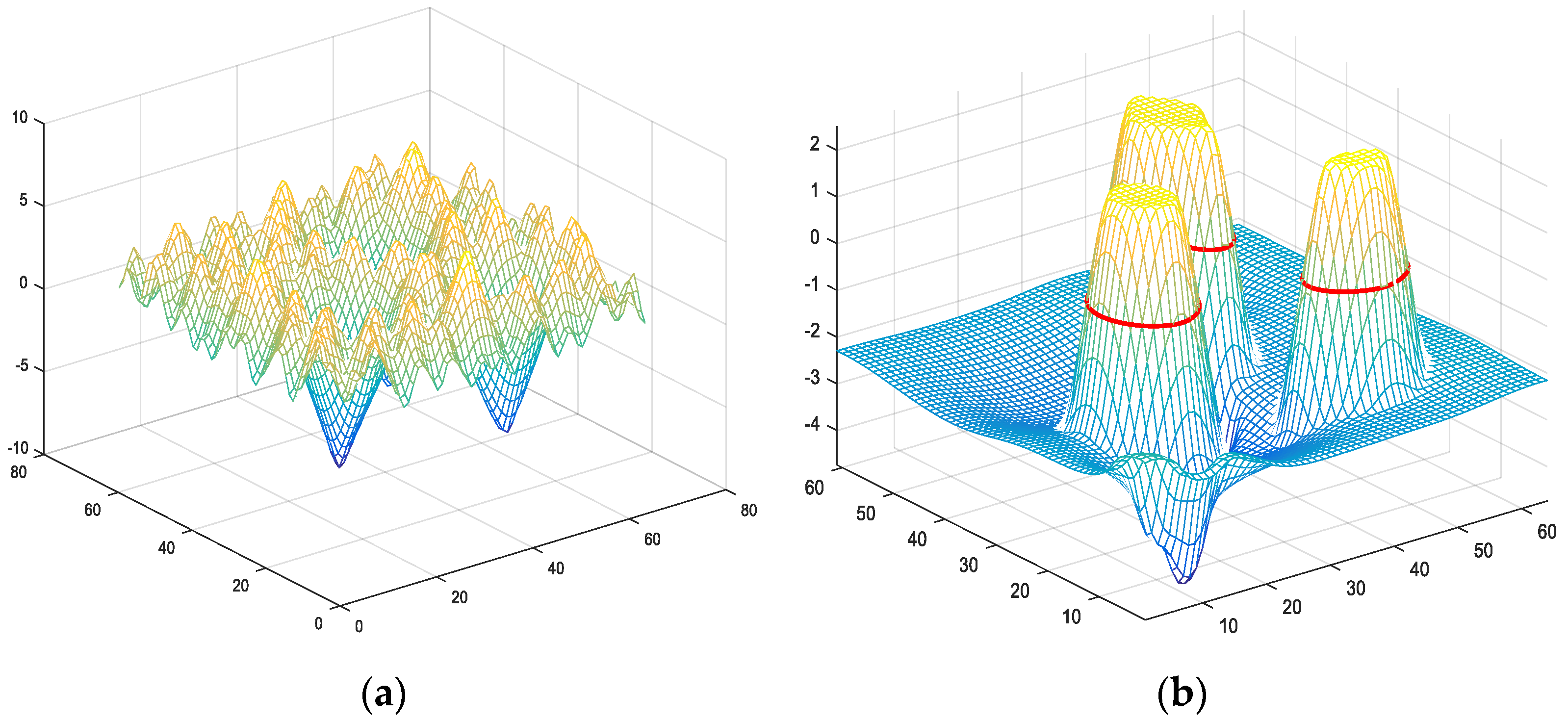
It can be seen from Equation (21) that when $\left|\nabla \varphi \right|=1$, $r_1=0$ is in a stable state; when $\left|\nabla \varphi \right|=0$, $r_1=1$ is also in a stable state. Therefore, under the action of the double-well potential function, the final level set function is relatively smoother, as shown in Figure 2.

The gradient descent flow equation of the level set function $\varphi$ obtained by minimizing the energy functional (20) is as follows,

$$\frac{\partial \varphi }{\partial t}=\mu \mathrm{div}(d_R\left|\nabla \varphi \right|\cdot \nabla \varphi ),$$

(22)

where the function $d_R$ is defined as Equation (7).

4.2. Regularization Term $E^R$

The second term in the Equation (19) is a regular term, which is used to maintain the regularity of the evolution curve and calculate the line integral of the curve. The energy function is as follows,

$$E^R=\nu {\displaystyle {\iint }_{\mathrm{\Omega }}g(x,y)(\left|\nabla H(\varphi )\right|)}dxdy,$$

(23)

where $\nu >0$ is the weight coefficient, and $g(x,y)$ is the fractional edge-stopping function, as shown in Equation (18) and described in detail in Section 3.

The gradient downflow equation of the level set function $\varphi$ is obtained by minimizing the energy functional (23) as follows,

$$\frac{\partial \varphi }{\partial t}=\nu g\delta (\varphi )\cdot \mathrm{div}(\frac{\nabla \varphi }{\left|\nabla \varphi \right|}).$$

(24)

Due to the introduction of a fractional-order edge-stopping function in this term, the model has a certain robustness to noise. The improved fractional-order edge-stopping function only relies on the gradient information of the image and cannot solve the problem that the model is sensitive to the initial contour position. Therefore, in Section 4.3, the adaptive fractional derivative is introduced into the region fitting term, and the use of the fractional derivative can enhance the advantages of the image texture details and optimize the segmentation method.

4.3. Fitting Term $E^F$

The third term in the Equation (19) is a fitting term, which is used to drive the evolution curve to stop at the target contour and make the model robust to the initial contour position. The fitting term proposed in this paper includes two parts: one is the local region fitting term introduced from [24], and the other is the fitting term based on the adaptive fractional differential. The energy functional is as follows,

$$\begin{array}{ll}{E}^F=& \lambda [{\displaystyle {\iint }_{\mathrm{\Omega }}{K}_{\sigma }(x-y){(I(y)-f_1(x))}^{2}H(\varphi (y))dxdy}\\ & +{\displaystyle {\iint }_{\mathrm{\Omega }}{K}_{\sigma }(x-y){(I(y)-f_2(x))}^2(1-H(\varphi (y)))dxdy}]\\ & +E^{FF}\end{array}$$

(25)

where $f_1(x)$ and $f_2(x)$ are respectively the fitting mean of the local area inside and outside the contour curve of a given pixel point $x$, and the expression is Equation (9). $K_{\sigma }(x)$ is the Gaussian kernel function with standard deviation $\sigma$, $I(y)$ is the intensity of the image $I(x,y)$ at point $y$, $\varphi (y)$ is the level set function at a point $y$, and $\delta (\cdot )$ and $H(\cdot )$ are Equations (4) and (5).

The energy function of the fitting term $E^{FF}$, based on adaptive fractional differentiation is,

$$\begin{array}{ll}{E}^{FF}=& \gamma [{\displaystyle {\iint }_{\mathrm{\Omega }}{K}_{\sigma }(x-y){(FI(y)-b_1(x))}^{2}H(\varphi (y))dxdy}\\ & +{\displaystyle {\iint }_{\mathrm{\Omega }}{K}_{\sigma }(x-y){(FI(y)-b_2(x))}^2(1-H(\varphi (y)))dxdy}]\end{array}$$

(26)

where $b_1(x)$ and $b_2(x)$ are the local area fitting means of the given pixel x inside and outside the contour curve, respectively,

$$b_i(x)=\frac{K_{\sigma }(x)\cdot [H_i(\varphi (x))FI(x)]}{K_{\sigma }(x)\cdot H_i(\varphi (x))} i=1,2.$$

(27)

Among them, $FI(x,y)$ is the image $I(x,y)$ after adaptive fractional differential processing. The specific derivation can be obtained from Equation (17) and is described in detail in Section 3.2,

$$FI(x,y)=I(x,y)+\left|{}^{GL}\mathcal{D}^{P}I(x,y)\right|.$$

(28)

The gradient descent flow equation of the level set function $\varphi$ obtained by minimizing the energy functional (25) is as follows,

$$\begin{array}{ll}\frac{\partial \varphi }{\partial t}=& -\lambda \delta (\varphi )[{\displaystyle \int K_{\sigma }(x-y){(I(y)-f_1(x))}^2}dx\\ & -{\displaystyle \int K_{\sigma }(x-y){(I(y)-f_2(x))}^2}dx]\\ & -\gamma \delta (\varphi )[{\displaystyle \int K_{\sigma }(x-y){(FI(y)-b_1(x))}^2}dx\\ & -{\displaystyle \int K_{\sigma }(x-y){(FI(y)-b_2(x))}^2}dx]\end{array}$$

(29)

Finally, the gradient descent flow equation by minimizing the level set function $\varphi$ of the total energy functional (19) in this paper is as follows,

$$\begin{array}{ll}\frac{\partial \varphi }{\partial t}=& \mu \mathrm{div}(d_R\left|\nabla \varphi \right|\cdot \nabla \varphi )+\nu g\delta (\varphi )\cdot \mathrm{div}(\frac{\nabla \varphi }{\left|\nabla \varphi \right|})\\ & -\lambda \delta (\varphi )[{\displaystyle \int K_{\sigma }(x-y){(I(y)-f_1(x))}^2}dx\\ & -{\displaystyle \int K_{\sigma }(x-y){(I(y)-f_2(x))}^2}dx]\\ & -\gamma \delta (\varphi )[{\displaystyle \int K_{\sigma }(x-y){(FI(y)-b_1(x))}^2}dx\\ & -{\displaystyle \int K_{\sigma }(x-y){(FI(y)-b_2(x))}^2}dx]\end{array}$$

(30)

Then the level set evolution equation in Equation (30) can be discretized as,

$$\frac{{\varphi }_{i,j}^{{}^{n+1}}-{\varphi }_{i,j}^{{}^n}}{\Delta t}=L({\varphi }_{i,j}^{{}^n}),$$

(31)

where $(i,j)$ is the spatial index, $k$ is the time index, and $L({\varphi }_{i,j}^{{}^n})$ is the numerical approximation of the function on the right side of the evolution Equation (31).

The iterative equation of the level set function can be expressed as,

$${\varphi }_{i,j}^{{}^{n+1}}={\varphi }_{i,j}^{{}^n}+\Delta t\cdot L({\varphi }_{i,j}^{{}^n}).$$

(32)

4.4. Implementation and Algorithm

The implementation and algorithm steps of the active contour model of image segmentation, based on adaptive fractional differentiation proposed in this paper, are as follows:

Step1: Input the image $I(x,y)$, initialize the level set function, and set the initial parameter values: $\mu =0.2$, $\nu =1.5$, $\lambda =\gamma =1$, $\Delta t=5$, $\sigma =3$, $\epsilon =1.5$.

Step2: Calculate the result ${}^{GL}\mathcal{D}^{P}I(x,y)$ after the adaptive fractional differential operation from the Equation (15) in Section 3.2, and update the image $I(x,y)$ according to the Equation (17).

Step3: Calculate the fractional-order edge-stopping function $g(x,y)$ from the Equation (18) in Section 3.3.

Step4: Calculate the penalty term energy function $E^P$ from the Equation (20) in Section 4.1.

Step5: Calculate the energy function of the regular term $E^R$ by the Equation (23) in Section 4.2.

Step6: Calculate the energy function of the fitting term $E^{FF}$ based on the adaptive fractional differential by the Equation (26) in Section 4.3, and then calculate the energy function of the total fitting term $E^F$ by the Equation (25).

Step7: Calculate the gradient descent flow equation $\partial \varphi /\partial t$ of the level set function $\varphi$ of the total energy function $E$ by the Equation (30) in Section 4.3.

Step8: Calculate from the Equation (32) in Section 4.3, and update the level set function ${\varphi }^{n+1}(x)$ and ${\varphi }^n(x)$.

Step9: Check whether the set number of iterations is reached. If the number of iterations is reached, the curve stops evolving to output the final target contour; otherwise, return to Step 2.

Algorithm The algorithm for solving the proposed model

Input:$\mathrm{Infrared} \mathrm{image} I(x,y)\in n\times m$.

Output: Image segmentation results.

1: Set initialization parameters: $\mu ,\nu ,\lambda ,\gamma ,\Delta t,\sigma ,\epsilon ,{\mathit{Iter}}_{\max }$;

2: $\mathrm{Calculate} {}^{GL}\mathcal{D}^{P}I(x,y)$ by Equation (16);

3: for$n=1:Ite{r}_{\max }$ do

4: $\mathrm{Calculate} \mathrm{the} \mathrm{penalty} \mathrm{term} \mathrm{energy} \mathrm{function} E^P$ by Equation (20);

5: $\mathrm{Calculate} \mathrm{the} \mathrm{regularization} \mathrm{term} \mathrm{energy} \mathrm{function} E^R$ by Equation (23);

6: Calculate the fitting term energy function $E^F$ by Equation (25);

7: $\mathrm{Calculate} \mathrm{the} \mathrm{gradient} \mathrm{descent} \mathrm{flow} \mathrm{equation} \partial \varphi /\partial t$ of the total energy function $E$ by Equation (30);

8: Update the level set function ${\varphi }^{n+1}(x)$$\mathrm{and} {\varphi }^n(x)$ by Equation (32);

9: if $n=={\mathit{Iter}}_{\max }$ then

10: break;

11: end if

12: end for

5. Experimental Results

In this section, the experimental contents are the robustness verification to noise, the robustness verification of the initial contour position, the comparison between fixed-order and adaptive differentiation, and the comparison with other methods (CV, RSF, Ref. [39], Ref. [40]). The computer configuration used in the experiment is an Intel CORE i5 processor, 8 GB memory, Windows 10 operating system, and the experimental platform MATLAB (R2016a).

In this paper, dice similarity coefficient (DSC) and intersection over union (IOU) are selected as performance evaluation indicators,

$$\mathrm{DSC}(A,B)=\frac{2\left|R_A\cap R_B\right|}{\left|R_A\right|+\left|R_B\right|},$$

(33)

$$\mathrm{IOU}(A,B)=\frac{\left|R_A\cap R_B\right|}{\left|R_A\cup R_B\right|}.$$

(34)

The segmentation results were quantitatively compared with the expert manual segmentation results, and the area-based DSC index and the IOU overlap performance index were used for comparison. Among them, $\left|\cdot \right|$ is the number of pixels, $R_A$ and $R_B$ are the expert segmentation area and the experimental segmentation result area respectively. The closer the DSC and IOU values are to 1, the higher the segmentation accuracy.

5.1. Verify the Robustness of Noise

To verify that the active contour image segmentation method based on adaptive fractional differentiation proposed in this paper has good noise resistance, this section will conduct verification experiments on different types of noisy images.

In Figure 3, the infrared thermal image of candle burning is taken as the experimental object. From top to bottom are the original image, the noise image with Gaussian noise, speckle noise, and mixed noise. The mixed noise includes Gaussian noise and speckle noise, and the noise density is 0.03. From left to right are the noisy image, CV, RSF, Ref. [39], Ref. [40], and our method. The red rectangle in Figure 3a represents the initial contour, and the green curve in (b–f) represents the evolution result of the contour curve. The number of iterations of this experiment is $Ite{r}_{\max }=20$.

As shown in Figure 3b–e, the segmentation result is affected by noise to varying degrees, and some noise points are mistakenly considered as edges of the image. From the segmentation results in Figure 3f, it can be seen that the method proposed in this paper obtain better segmentation results under three types of noise conditions. These results show that the Gaussian kernel in the local fitting term is effective in dealing with the noise of the evolution process.

In addition to visual effects, IOU and DSC performance index values under different models in

Table 1. Corresponding evaluation index values.

Noise Image	Performance Index	Models
		CV	RSF	Ref. [39]	Ref. [40]	Ours
Clear	IOU	0.9146	0.9033	0.8153	0.7104	0.9856
	DSC	0.9368	0.9492	0.8983	0.8307	0.9927
Gaussian	IOU	0.9183	0.8678	0.7540	0.8109	0.9814
	DSC	0.9335	0.9292	0.8598	0.8955	0.9898
Speckle	IOU	0.9276	0.7696	0.8058	0.7125	0.9714
	DSC	0.9431	0.8698	0.8925	0.8321	0.9898
Gaussian + Speckle	IOU	0.9222	0.7813	0.7428	0.7310	0.9687
	DSC	0.9402	0.8772	0.8524	0.8446	0.9930

were also compared. It can be seen that our model can obtain better performance indicators and segmentation results.

5.2. Initial Contour Position Robustness Verification

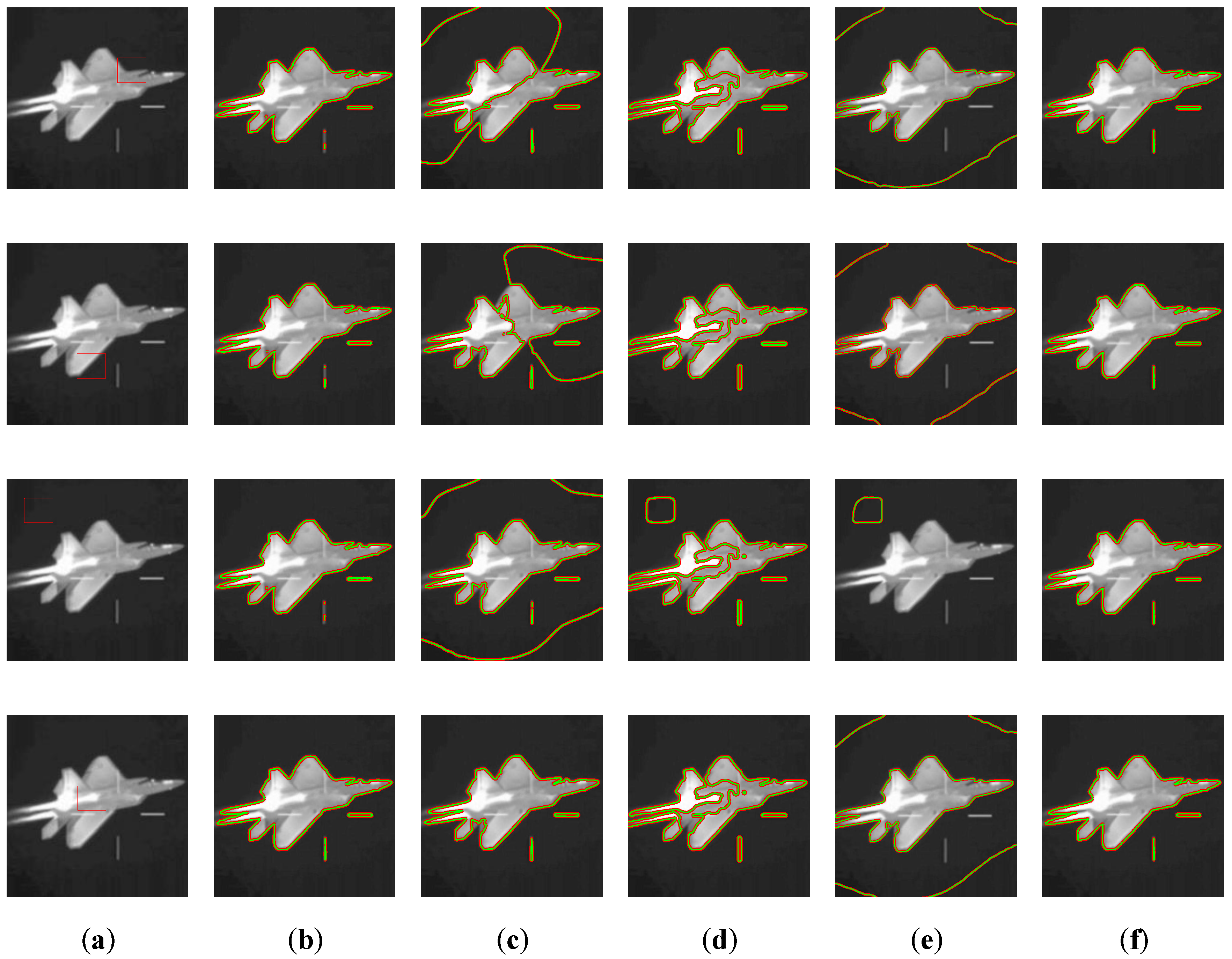
In this section, test experiments are used to verify the robustness of the proposed model to the initial curve, and the infrared image of the aircraft is taken as the experimental object. Figure 4 shows the segmentation results of different models and the proposed method for non-uniform images with different initial shapes. In Figure 4, from left to right are the input image, CV, RSF, Ref. [39], Ref. [40], and the proposed method where the input image has initial contours at different locations. In addition, the evolution process diagram of the level set function of different models is shown inFigure 5, which verifies the stability of the level set function of the model in this paper during the evolution process. The red rectangle in Figure 4a represents the initial contour, and the green curve in (b–f) represents the evolution result of the contour curve. The number of iterations of this experiment is $Ite{r}_{\max }=40$.

The results in Figure 4c–e show that the three models are sensitive to the initial contour position and often fail to achieve ideal segmentation results due to improper initial conditions. In Figure 4b–e, the CV model and the method in this paper can obtain similar results under different initial conditions. It is verified that our model is robust to the position of the initialization contour. In Figure 5a–d, the level set functions of other models will become more and more irregular in the iteration process, leading to oscillation in the evolution process, and then the accuracy of calculation will be seriously affected. Finally, the stability of level set evolution will be destroyed. In Figure 5e under the action of the double-well potential function, the final level set function is relatively smoother, which is conducive to the stability of the model.

5.3. Comparison between Fixed Order and Adaptive Differential

In this subsection, we will segment images with blurred object edges, and verify the performance of combining local region fitting and adaptive fractional differentiation in image segmentation. Furthermore, we validate the constraints on the correction parameters in adaptive fractional differentiation.

In the segmentation results in Figure 6, there are five different infrared images Pic 1–Pic 5 from top to bottom. The image contents are aircraft, human arms, and daily living environment. From left to right are the input image and initial contour, ordinary integer-order differential, 0.8-order fixed-order fractional differential, and our method. The red rectangle in Figure 6a represents the initial contour, and the green curve in (b–d) represents the evolution result of the contour curve. The number of iterations of this experiment is $Ite{r}_{\max }=40$.

The above is the segmentation result and performance index after processing the infrared grayscale image. Figure 6b shows that for infrared images with large background noise and blurred visual effects, ordinary integer order differential is easy to fall into a local minimum. In Figure 6c, a 0.8-order fixed-order fractional order G-L differential is adopted, and the same order differential processing is performed in the low-frequency part and the high-frequency part of the image, resulting in smooth texture details of the image. Therefore, compared with ordinary integer order differentials, the segmentation result and performance index are poor. In Figure 6d, after adding the adaptive fractional local region fitting term, we observe it has certain robustness to noise, can effectively separate the background and the target, and is more noise resistant. At the same time, due to the adaptive fractional differentiation for different parts of texture details, more target details of the image can be extracted, and a better image segmentation effect is achieved.

Table 2. Corresponding evaluation index values are in Figure 6.

Image	Performance Index	Models
		General Derivative	Fixed Order	Adaptive Order
Pic1	IOU	0.9881	0.9798	0.9896
	DSC	0.9940	0.9898	0.9948
Pic2	IOU	0.9792	0.9722	0.9846
	DSC	0.9895	0.9859	0.9923
Pic3	IOU	0.8465	0.8200	0.9760
	DSC	0.9169	0.9001	0.9878
Pic4	IOU	0.9532	0.9680	0.9748
	DSC	0.9760	0.9838	0.9900
Pic5	IOU	0.9688	0.7847	0.9760
	DSC	0.9842	0.8794	0.9878

also shows the effectiveness of this method in terms of evaluation index values.

In addition, [32,33,34] solved the optimal control problem of nonlinear fractional order systems through gradient-based optimization methods. In this paper, the nonlinear parameter optimization strategy is used to process the modified parameters $\alpha$ and $\beta$, taking the performance indicators IOU and DSC as the objective function, and the modified parameter $\alpha ,\beta$ as the input variables, taking random values in $[0,1]$, and finally obtaining the optimal values of IOU and DSC. In Figure 7, the corresponding IOU and DSC values of the correction parameters under random values are shown respectively.

Figure 7 shows that for infrared images, when $\alpha >\beta$, the image segmentation performance IOU and DSC values are better than $\alpha <\beta$. Therefore, in the order matrix $P$ with adaptive order change, the constraint condition $\alpha >\beta$ of its modified parameters is established; in combination with the highest points of Figure 7a,b, the optimal values of $\alpha$ and $\beta$ are 1 and 0.8 respectively. Next, this paper selects those $\alpha$ and $\beta$ values of the best and non-best in Figure 7, processes different infrared images, and compares their processing effects in the edge part. In Figure 8, from left to right, there are seven different infrared images, including human body movements, flames when candles burn, aircraft, and daily living environment. From top to bottom are the input image, the nonoptimal segmentation result, and the optimal segmentation result. The red rectangle in the first row of images represents the initial contour, and the green curve in the second and third rows of images represents the evolution result of the contour curve.

The results in Figure 8 show that, for infrared images, the best correction parameters enable the method in this paper to obtain finer edge contours and show better results.

5.4. Compare with Other Methods

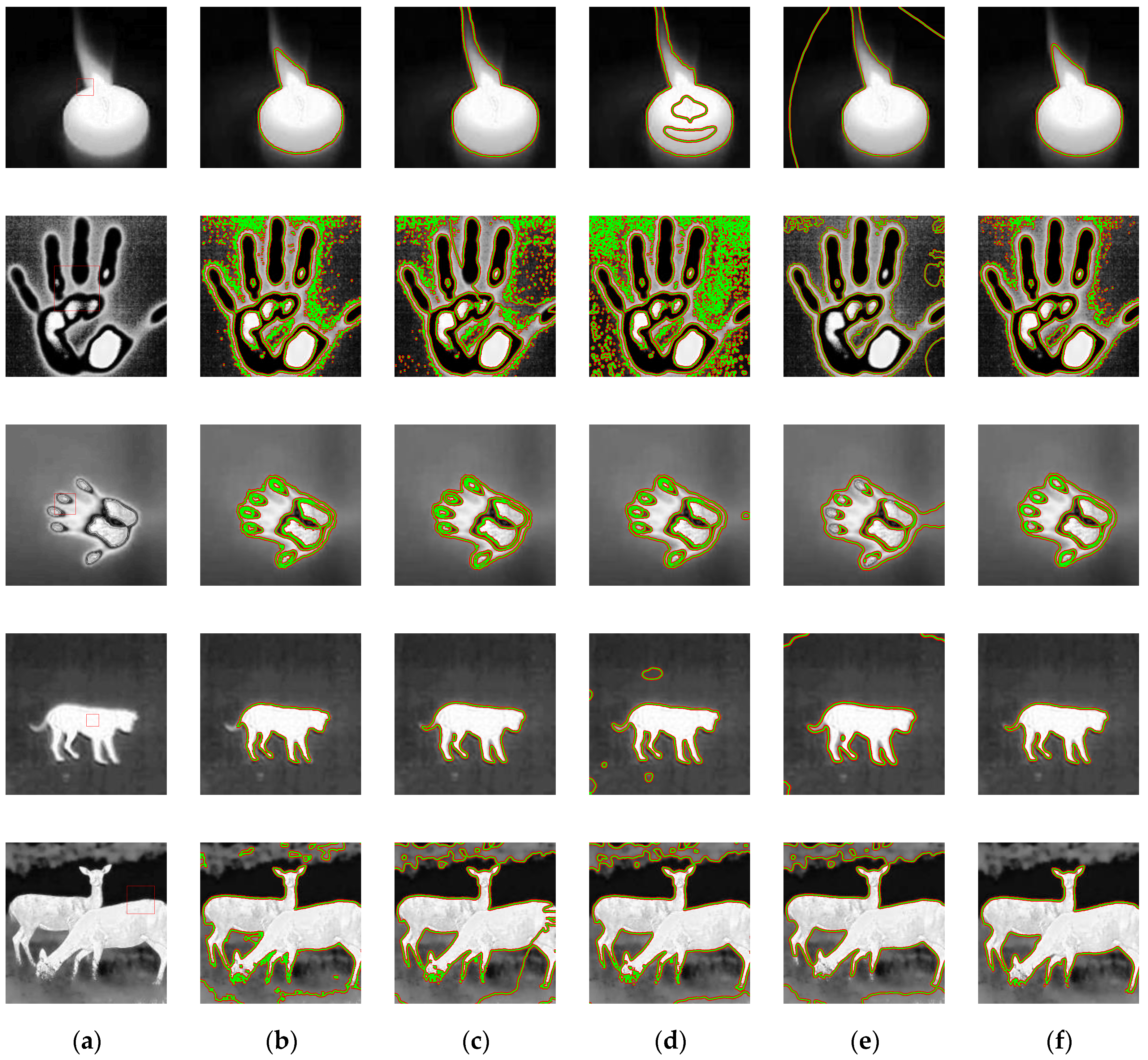
In this subsection, we compare the proposed model with CV, RSF, Ref. [39], and Ref. [40]. The effectiveness of the proposed model in processing noisy and uneven grayscale infrared images is verified. In Figure 9, there are five different infrared images Pic6–Pic10 from top to bottom. The image content is the infrared thermal image of burning candles, human palms, and animals. From left to right are the input image and the segmentation results of the initial contour, CV, RSF, Ref. [39], Ref. [40], and the proposed model in this paper, respectively. The red rectangle in Figure 9a represents the initial contour, and the green curve in (b–d) represents the evolution result of the contour curve. The number of iterations of this experiment is $Ite{r}_{\max }=40$.

The above is the segmentation result and performance index after processing the infrared thermal image. Figure 9b–e show that for infrared images with large background noise and blurred visual effect, the four models are easily affected by noise and initial contour position, and finally fall into the local minimum value. In Figure 9f, the method proposed in this paper can effectively separate the background from the target, has more noise resistance, extracts more target details of the image, and achieves a better image segmentation effect. It is shown in

Table 3. Performance index values corresponding to Figure 9.

Image	Performance Index	Models
		CV	RSF	Ref. [39]	Ref. [40]	Ours
Pic6	IOU	0.8781	0.9059	0.7293	0.5759	0.9832
	DSC	0.9351	0.9506	0.8435	0.7309	0.9915
Pic7	IOU	0.6245	0.5139	0.4482	0.3717	0.7101
	DSC	0.7689	0.6789	0.6190	0.5420	0.8579
Pic8	IOU	0.9331	0.6589	0.6410	0.5809	0.9510
	DSC	0.9654	0.7944	0.7812	0.7349	0.9749
Pic9	IOU	0.8125	0.8647	0.8309	0.8256	0.9929
	DSC	0.8966	0.9275	0.9077	0.9045	0.9965
Pic10	IOU	0.7527	0.6988	0.7135	0.6666	0.9539
	DSC	0.8589	0.8227	0.8328	0.7999	0.9764

that when fractional variable order differential processing is adopted, our model can obtain finer edge contours and better handle some details compared with other models. At the same time, it can also reflect the effectiveness of this model in evaluating the index value.

6. Conclusions

In this paper, an adaptive fractional differential active contour image segmentation method is proposed. Adaptive fractional differentiation is adopted to extract more textured parts from the image by adaptive order differentiation for each pixel. The fractional edge-stopping function improves noise resistance. Additionally, the fitting term based on adaptive fractional differentiation solves the problem that improper selection of the initial contour position will lead to inaccurate segmentation results. The experimental results show that for the infrared image with strong noise and blurred edges, this method can solve the problems of being sensitive to noise and initial contour position, and effectively segment the image of the weak edge target. In future research work, we will explore adaptive weighting techniques to achieve faster calculations and use fewer parameters and construct a better-performing active contour model for image segmentation.

References

1. Kass, M.; Witkin, A.; Terzopoulos, D. Snakes: Active contour models. Int. J. Comput. Vis. 1988, 1, 321–331. [Google Scholar] [CrossRef]
2. Lv, H.; Zhang, Y.; Wang, R. Active contour model based on local absolute difference energy and fractional-order penalty term. J. Appl. Math. Model. 2022, 107, 207–232. [Google Scholar] [CrossRef]
3. Jin, R.; Weng, G. Active contours driven by adaptive functions and fuzzy c-means energy for fast image segmentation. J. Signal Process. 2019, 163, 1–10. [Google Scholar] [CrossRef]
4. Lv, H.; Zhang, F.; Wang, R. Robust active contour model using patch-based signed pressure force and optimized fractional-order edge. J. IEEE Access 2021, 9, 8771–8785. [Google Scholar] [CrossRef]
5. Wei, X.; Zheng, W.; Xi, C.; Shang, S. Shoreline extraction in SAR image based on advanced geometric active contour model. J. Remote Sens. 2021, 13, 642. [Google Scholar] [CrossRef]
6. Karami, E.; Shehata, M.S.; Smith, A. Adaptive polar active contour for segmentation and tracking in ultrasound videos. J. IEEE Trans. Circuits Syst. Video Technol. 2018, 29, 1209–1222. [Google Scholar] [CrossRef]
7. Hu, P.; Wang, G.; Kong, X.; Kuen, J.; Tan, Y.-P. Motion-guided cascaded refinement network for video object segmentation. In Proceedings of the IEEE Conference on Computer Vision and Pattern Recognition, Salt Lake City, UT, USA, 18–22 June 2018; pp. 1400–1409. [Google Scholar]
8. Zhang, P.; Liu, W.; Lei, Y.; Wang, H.; Lu, H. Deep multiphase level set for scene parsing. J. IEEE Trans. Image Process. 2020, 29, 4556–4567. [Google Scholar] [CrossRef] [Green Version]
9. Yang, S.; Wu, J.; Feng, Z. Dual-Fusion active contour model with semantic information for saliency target extraction of underwater images. J. Appl. Sci. 2022, 12, 2515. [Google Scholar] [CrossRef]
10. Pan, Z.; Liu, S.; Fu, W. A review of visual moving target tracking. J. Multimed. Tools Appl. 2017, 76, 16989–17018. [Google Scholar] [CrossRef]
11. Lobregt, S.; Viergever, M.A. A discrete dynamic contour model. J. IEEE Trans. Med. Imaging 1995, 14, 12–24. [Google Scholar] [CrossRef]
12. Bendaoud, A.; Hachouf, F. Fractional calculus for improving edge-based active contour models. In Proceedings of the 2021 International Conference on Recent Advances in Mathematics and Informatics (ICRAMI), Tebessa, Algeria, 21–22 September 2021; IEEE: Piscataway, NJ, USA, 2021; pp. 1–5. [Google Scholar]
13. Liu, C.; Liu, W.; Xing, W. An improved edge-based level set method combining local regional fitting information for noisy image segmentation. J. Signal Process. 2017, 130, 12–21. [Google Scholar] [CrossRef]
14. Yu, H.; He, F.; Pan, Y. A novel segmentation model for medical images with intensity inhomogeneity based on adaptive perturbation. J. Multimed. Tools Appl. 2019, 78, 11779–11798. [Google Scholar] [CrossRef]
15. Liu, C.; Liu, W.; Xing, W. A weighted edge-based level set method based on multi-local statistical information for noisy image segmentation. J. Vis. Commun. Image Represent. 2019, 59, 89–107. [Google Scholar] [CrossRef]
16. Yang, Y.; Hou, X.; Ren, H. Efficient active contour model for medical image segmentation and correction based on edge and region information. J. Expert Syst. Appl. 2022, 194, 116436. [Google Scholar] [CrossRef]
17. Li, M.; Zhan, Y.; Ge, Y. Fractional distance regularized level set evolution with its application to image segmentation. J. IEEE Access 2020, 8, 84604–84617. [Google Scholar] [CrossRef]
18. Chen, B.; Huang, S.; Liang, Z.; Chen, W.; Pan, B. A fractional order derivative based active contour model for inhomogeneous image segmentation. J. Appl. Math. Model. 2019, 65, 120–136. [Google Scholar] [CrossRef]
19. Yan, X.; Weng, G. Hybrid active contour model driven by optimized local pre-fitting image energy for fast image segmentation. J. Appl. Math. Model. 2022, 101, 586–599. [Google Scholar] [CrossRef]
20. Fang, J.; Liu, H.; Zhang, L.; Liu, J.; Liu, H. Region-edge-based active contours driven by hybrid and local fuzzy region-based energy for image segmentation. J. Inf. Sci. 2021, 546, 397–419. [Google Scholar] [CrossRef]
21. Caselles, V.; Kimmel, R.; Sapiro, G. Geodesic active contours. Int. J. Comput. Vis. 1997, 22, 61–79. [Google Scholar] [CrossRef]
22. Li, C.; Xu, C.; Gui, C.; Fox, M.D. Level set evolution without re-initialization: A new variational formulation. In Proceedings of the 2005 IEEE Computer Society Conference on Computer Vision and Pattern Recognition (CVPR’05), San Diego, CA, USA, 20–25 June 2005; IEEE: Piscataway, NJ, USA, 2005; pp. 430–436. [Google Scholar]
23. Chan, T.F.; Vese, L.A. Active contours without edges. J. IEEE Trans. Image Process. 2001, 10, 266–277. [Google Scholar] [CrossRef] [PubMed]
24. Li, C.; Kao, C.-Y.; Gore, J.C.; Ding, Z. Minimization of region-scalable fitting energy for image segmentation. J. IEEE Trans. Image Process. 2008, 17, 1940–1949. [Google Scholar]
25. Zhang, X.; Liu, R.; Ren, J.; Gui, Q. Adaptive fractional image enhancement algorithm based on rough set and particle swarm optimization. J. Fractal Fract. 2022, 6, 100. [Google Scholar] [CrossRef]
26. Yan, H.; Zhang, X. Adaptive fractional multi-scale edge-preserving decomposition and saliency detection fusion algorithm. J. ISA Trans. 2020, 107, 160–172. [Google Scholar] [CrossRef]
27. Zhang, X.; Dai, L. Image enhancement based on rough set and fractional order differentiator. J. Fractal Fract. 2022, 6, 214. [Google Scholar] [CrossRef]
28. Yan, H.; Zhang, J.-X.; Zhang, X. Injected infrared and visible image fusion via L1 decomposition model and guided filtering. J. IEEE Trans. Comput. Imaging 2022, 8, 162–173. [Google Scholar] [CrossRef]
29. Khanna, S.; Chandrasekaran, V. Fractional differentiation-based edge energy driven active contours for robust image segmentation. ICTACT J. Image Video Process. 2021, 12, 2493–2501. [Google Scholar]
30. Zhang, Y.; Tian, Y. A new image segmentation method based on fractional-varying-order differential. J. Beijing Inst. Technol. 2021, 30, 254–264. [Google Scholar]
31. Li, M.-M.; Li, B.-Z. A novel active contour model for noisy image segmentation based on adaptive fractional order differentiation. J. IEEE Trans. Image Process. 2020, 29, 9520–9531. [Google Scholar] [CrossRef]
32. Liu, C.; Gong, Z.; Yu, C.; Wang, S.; Teo, K.L. Optimal control computation for nonlinear fractional time-delay systems with state inequality constraints. J. Optim. Theory Appl. 2021, 191, 83–117. [Google Scholar] [CrossRef]
33. Gong, Z.; Liu, C.; Teo, K.L.; Yi, X. Optimal control of nonlinear fractional systems with multiple pantograph-delays. J. Appl. Math. Comput. 2022, 425, 127094. [Google Scholar] [CrossRef]
34. Gong, Z.; Liu, C.; Teo, K.L.; Wang, S.; Wu, Y. Numerical solution of free final time fractional optimal control problems. J. Appl. Math. Comput. 2021, 405, 126270. [Google Scholar] [CrossRef]
35. Zhang, X.; Yan, H. Medical image fusion and noise suppression with fractional-order total variation and multi-scale decomposition. J. IET Image Process. 2021, 15, 1688–1701. [Google Scholar] [CrossRef]
36. Zhang, X.; He, H.; Zhang, J.-X. Multi-focus image fusion based on fractional order differentiation and closed image matting. J. ISA Trans. 2022, in press. [Google Scholar] [CrossRef] [PubMed]
37. Li, C.; Xu, C.; Gui, C.; Fox, M.D. Distance regularized level set evolution and its application to image segmentation. J. IEEE Trans. Image Process. 2010, 19, 3243–3254. [Google Scholar] [CrossRef]
38. Aubert, G.; Kornprobst, P.; Aubert, G. Mathematical Problems in Image Processing: Partial Differential Equations and the Calculus of Variations; Springer: Berlin/Heidelberg, Germany, 2006; p. 147. [Google Scholar]
39. Ding, K.; Xiao, L.; Weng, G. Active contours driven by local pre-fitting energy for fast image segmentation. J. Pattern Recognit. Lett. 2018, 104, 29–36. [Google Scholar] [CrossRef]
40. Liu, H.; Fang, J.; Zhang, Z.; Lin, Y. A novel active contour model guided by global and local signed energy-based pressure force. J. IEEE Access 2020, 8, 59412–59426. [Google Scholar] [CrossRef]
Figure 1. Example of adaptive order matrix P with dimension 5 × 5 .
Fractalfract 06 00579 g001
Figure 2. Level set function. (a) Level set function in [22]; (b) level set function in [37].
Fractalfract 06 00579 g002
Figure 3. Segmentation results for different types of noise. (a) Input image and initial contour; (b) CV; (c) RSF; (d) Ref. [39]; (e) Ref. [40]; (f) Ours.
Fractalfract 06 00579 g003
Figure 4. Segmentation results in different initial contours. (a) Input image and initial contour; (b) CV; (c) RSF; (d) Ref. [39]; (e) Ref. [40]; (f) Ours.
Fractalfract 06 00579 g004
Figure 5. Level set functions for different models. (a) CV; (b) RSF; (c) Ref. [39]; (d) Ref. [40]; (e) Ours.
Fractalfract 06 00579 g005
Figure 6. Segmentation results in a fixed order and variable order. (a) Input image Pic 1–Pic 5 and initial contour; (b) General derivative; (c) Fixed order; (d) Adaptive order.
Fractalfract 06 00579 g006
Figure 7. Performance index value. (a) IOU value; (b) DSC value.
Fractalfract 06 00579 g007
Figure 8. Comparison of infrared image segmentation results between the best and non-best. (a) Infrared image of human motion in simple background; (b) Infrared image of human motion in complex background; (c) Infrared image of candle burning flame; (d) Infrared image of aircraft; (e) Infrared image of fighter; (f) Infrared image under complex background; (g) Infrared image under complex background.
Fractalfract 06 00579 g008
Figure 9. Segmentation results of infrared images. (a) Input image Pic6–Pic10 and initial contour; (b) CV; (c) RSF; (d) Ref. [39]; (e) Ref. [40]; (f) Ours.
Fractalfract 06 00579 g009