1. Introduction
Continuum mechanics of homogeneous media has been the basis of studies of shock formation due to sources moving faster than the speed of sound. Such studies belong to aerodynamics. However, if a generalization to heterogeneous media is considered, the subject of such shocks in random media would have its basis in a general field of waves in random media (or stochastic wave propagation). While various investigations have been carried out in this area, to the best of our knowledge, no studies of shock and Mach fronts due to sources moving in random media have ever been reported. In particular, random media with fractal (i.e., hierarchical-type multiscale) and Hurst (i.e., long-range memory) effects offer an additional difficulty.
The basic motivation for studying waves in such media comes from the fact that such geometric characteristics appear in nature, both in biological and geologic structures, as well as atmospheric turbulence [
1,
2,
3,
4]. In addition, ref. [
4] reported that heat conduction in a porcine muscle follows a damped wave equation of
second sound, and this finding is consistent with other studies, e.g., [
5,
6]. At present, it is not known whether this equation would also correctly model the heat transfer in electrosurgery, where a surgeon may cut a living tissue at several centimeters per second. However, given the observation that signals in soft tissues may travel slower than a surgeon’s hand, there may occur supersonic (or even hypersonic) heat propagation phenomena. Thus, the present paper is a stepping-stone in that direction.
Overall, this paper is organized as follows.
Section 2 gives the problem formulation in a stochastic framework.
Section 3 introduces the random field (RF) models of Cauchy and Dagum types.
Section 4 outlines the numerical treatment of the telegraph equation.
Section 5 gives the numerical results in terms of the animations of temperature fields and provides comparisons between such fields and the reference solution on a homogeneous medium. Finally,
Section 6 concludes this paper.
2. Problem Formulation
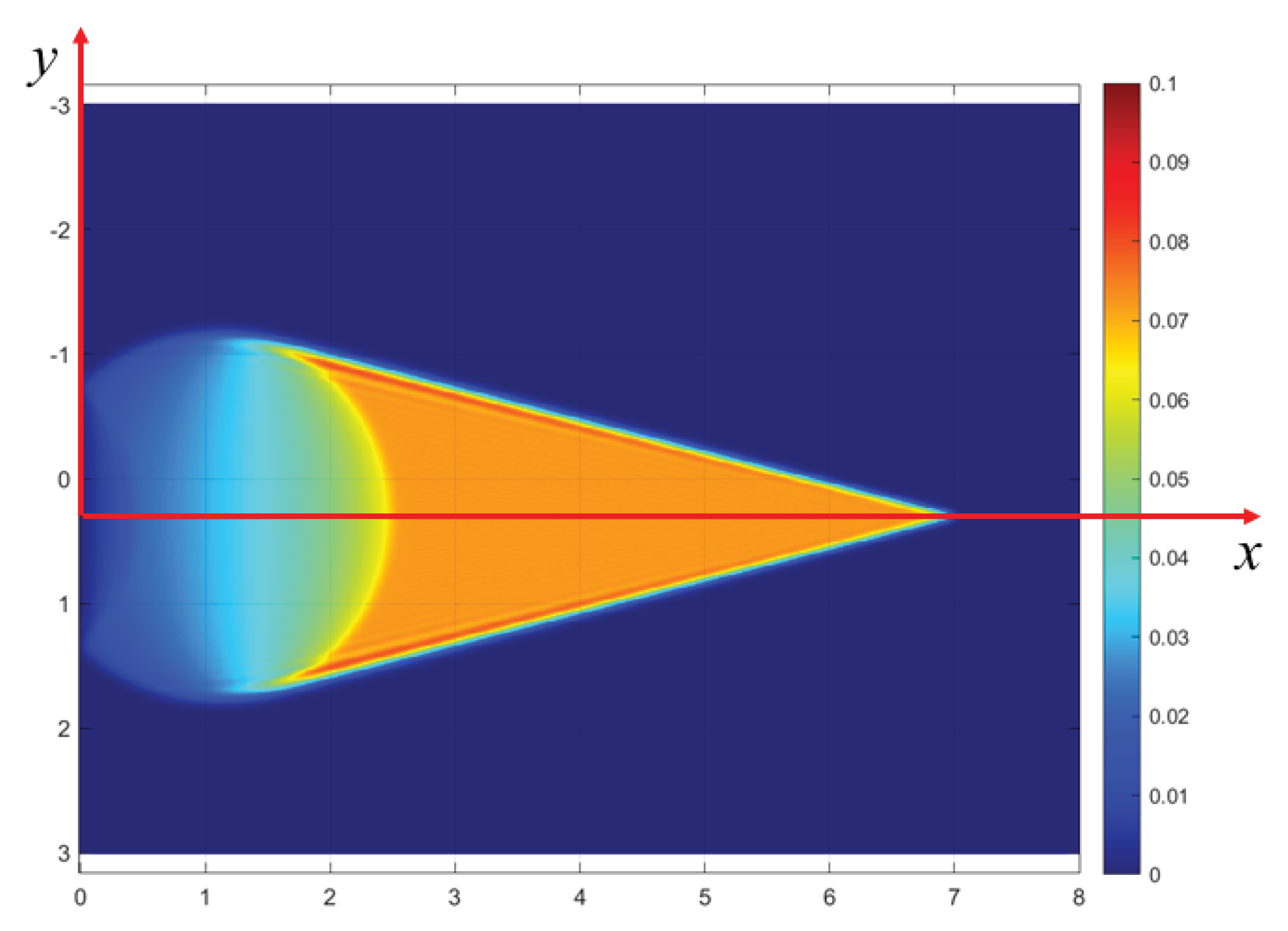
The investigation concerns second sound phenomena in two dimensions (2d), i.e., those governed by a telegraph partial differential equation for the temperature field
T in a planar body domain
B (
Figure 1).
where
is the Laplacian in the
-plane,
Q is the heat source,
the thermal diffusivity is taken
, while
, the relaxation time, is taken as a random field (RF). The second sound is a thermal wave resulting from the hypothesis that the temperature gradient is proportional not only to the heat flux (as in Fourier’s law) but also to the rate of heat flux multiplied by a relaxation time. As a result, the heat conduction is governed by a hyperbolic rather than a parabolic partial differential equation. The relaxation times are on the order of seconds and even tens of seconds in polymers [
4,
5,
6]. The hyperbolic transfer equation was first obtained by Fock [
7], followed by Davydov [
8], Cattaneo [
9,
10] and Vernotte [
11].
The RF
is taken according to a Reynolds decomposition:
In general, is an RF of position (), where is a realization drawn from a probability space .
We consider situations where
Q moves faster than the speed of second sound
c, implying the supersonic effects. Given that
,
c is a random field, so these effects are stochastic in space–time. Hence, the basic question is:
How are the Mach wedges affected by the medium having a random multiscale structure with long-range memory? Mathematically, the RF
is generated by employing Cauchy or Dagum correlation functions, where the fractal dimension
D and the Hurst parameter
H can be varied independently, i.e., without imposing the self-affine geometry [
12,
13]. Note that the conventional random process/field models such as white-noise or Ornstein–Uhlenbeck, while very common in the literature, do not exhibit these interesting effects.
From a general perspective, the present study continues our investigations of (i) structural mechanics problems, (ii) dynamical systems, (iii) waves and wavefronts and (iv) fracture on tensor-valued random fields (see, e.g., [
14]). Only in the simplest cases of (i) and (ii) are explicit analytical solutions possible, whereby we note that even the explicit spectra of Cauchy and Dagum models are formidable mathematical challenges. Therefore, we employ a computational approach to simulate realizations of RFs and then to solve for wave fields due to sources moving on such fields.
Generally, the governing field equation of deterministic continuum physics in a homogeneous medium can be written as
where
is a partial differential operator governing the second sound phenomenon; recall (1). If we introduce spatial randomness into the material properties appearing in the partial differential operator, then (3) is replaced by a stochastic field equation incorporating the spatial fluctuation
Here,
is a single realization of the sample space
which together with a
-algebra
S and a probability measure
P on it forms a probability space
. At this stage, a Gaussian measure will be assumed, although, if more information about the material randomness is available, other types of probability distribution are possible. The space
defines a random medium
. The ensemble average (i.e., the stochastic expectation) of
is
and, as always for stochastic systems, one is first interested in the average displacement response
before inquiring about the second and higher moments, and, ideally, about the probability distribution of the response. The above straightforward averaging of (
4) leads to a deterministic field equation
where
is the deterministic (and supposedly right...) solution. However, the correct average solution,
, of the stochastic problem (4) is formally obtained by first inverting (
4), then averaging, and then inverting again:
In general, there is no closed-form solution to (7). Therefore, the basic question of stochastic field theories is: If one replaces by , how different will the solutions and be?
In the following, we focus on a related issue from a geometric standpoint:
To determine the effect of random multiscale structure with long-range memory on the Mach wedges. This will be done by comparing the realizations of temperature RFs
in the random medium setting with the reference solution in the homogeneous reference medium defined by
. Effectively, since analytical solutions are impossible, the study method is of the Monte Carlo type. Note that the analytical solution elucidating the Doppler effect in the subsonic range of the second sound in a homogeneous 1d medium has recently been obtained [
15].
3. Random Fields
Since many conspicuous patterns in nature can be described by fractal geometry and Hurst characteristics, two RF models which can capture such effects are considered here: Cauchy and Dagum [
12,
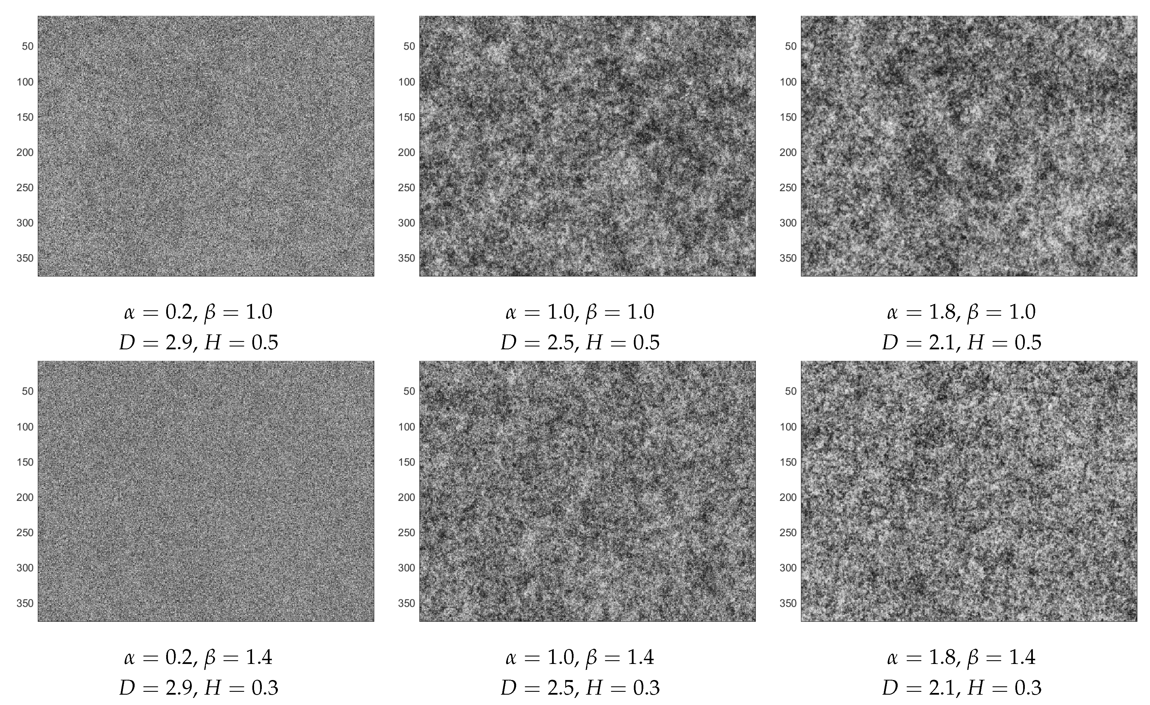
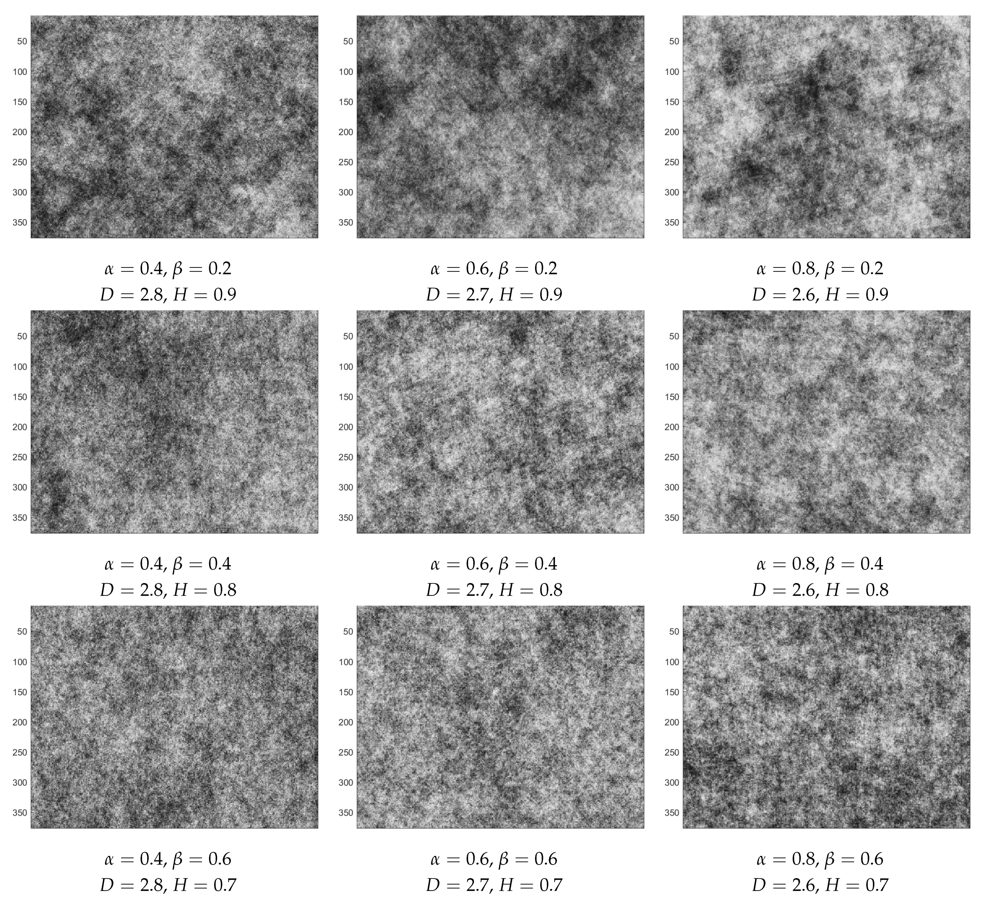
13]. Realizations of these RFs for a wide range of fractal dimension
D and Hurst parameter
H are displayed in
Figure 2 and
Figure 3. The fractal dimension denoted by
D is a roughness measure with
D for two-dimensional systems. A larger
D indicates a rougher surface. The Hurst parameter denoted by
H describes the long-range dependence. In general, an anti-persistent system is associated with
H , but a persistent system with
H . For reference, the case of
in a 1d RF (i.e., a random process), corresponds to a symmetric random walk without any long-range dependence.
The simplest model one can consider is the white noise RF (i.e., lacking any spatial correlations). Its covariance function is
where
is the Dirac delta function.
The covariance function for a Cauchy RF is
The covariance function for a Dagum RF is
Both Cauchy and Dagum RF models are capable of decoupling the fractal dimension
D from the Hurst coefficient
H; that is, one can independently choose
D and
H. With
n being the dimensionality of the material domain on which the RF is defined (i.e.,
for
), the relationships between
and
in these two covariance functions are given as
These two equations show that the parameters alpha and beta correspond (and control), respectively, the fractal dimension and the long memory. All the combinations of
and
for both Cauchy and Dagum RFs are generated using the RF package in
[
16]. It is a freeware environment for statistical computing and graphics providing, among others, a convenient tool for simulation of a wide range of random fields.
4. Numerical Treatment of Telegraph Equation
The problem to solve is:
where
is the heat point source moving at a constant speed
v = 2 cm/s in the
direction at level
(on the horizontal center line), and
is an RF.
To obtain the numerical solution, we first spatially discretize Equation (
12) on a
grid, where
= 0.016 cm, with the second-order central differencing:
This results in a second-order system in the form:
where
A is the Laplacian operator from above, and
C is the matrix containing material properties
at each grid point.
For the temporal discretization, we first reduce the system to first order in time by constructing a linear system:
where the first equation in (
15) is equivalent to Equation (
14) and the second equation is
;
I is the identity matrix. Thus, we are able to time-step the newly constructed vector
with its time derivative:
Upon inspection of the spectrum of L, through simple eigen-decompositions, we can see that it has imaginary eigenvalues, which is as expected from the hyperbolic nature of the equation, since the diffusion equation gives negative real eigenvalues and wave equation gives imaginary eigenvalues. Therefore, Runge–Kutta 4 is used as the time-stepper because its stability region covers the imaginary axis, with = 0.008 s where stability can be easily ensured.
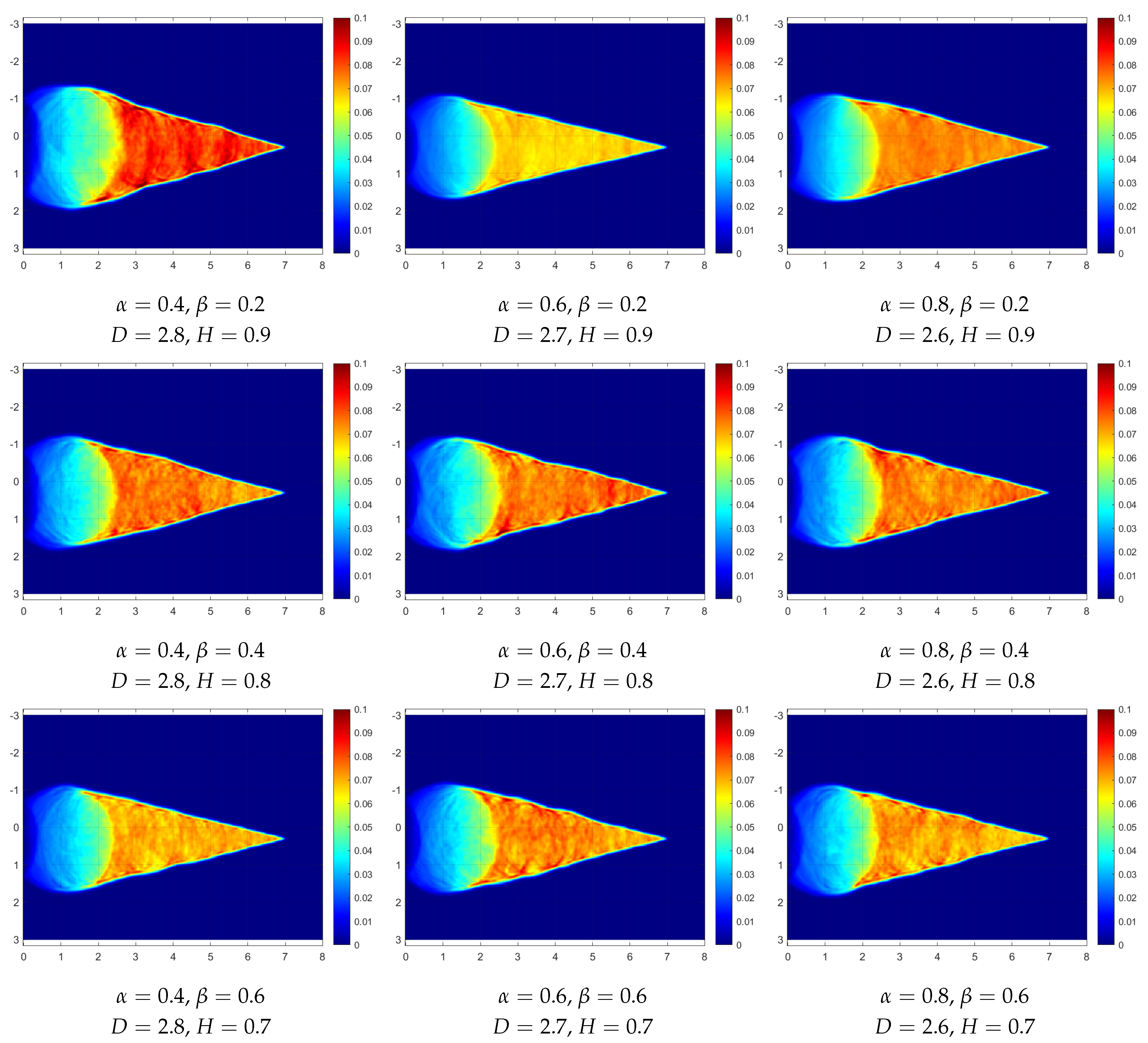
5. Simulation Results
This section reports temperature fields obtained from solving sample realizations of RFs of the property
. Simulations are performed in MATLAB with random fields generated by the RF package in
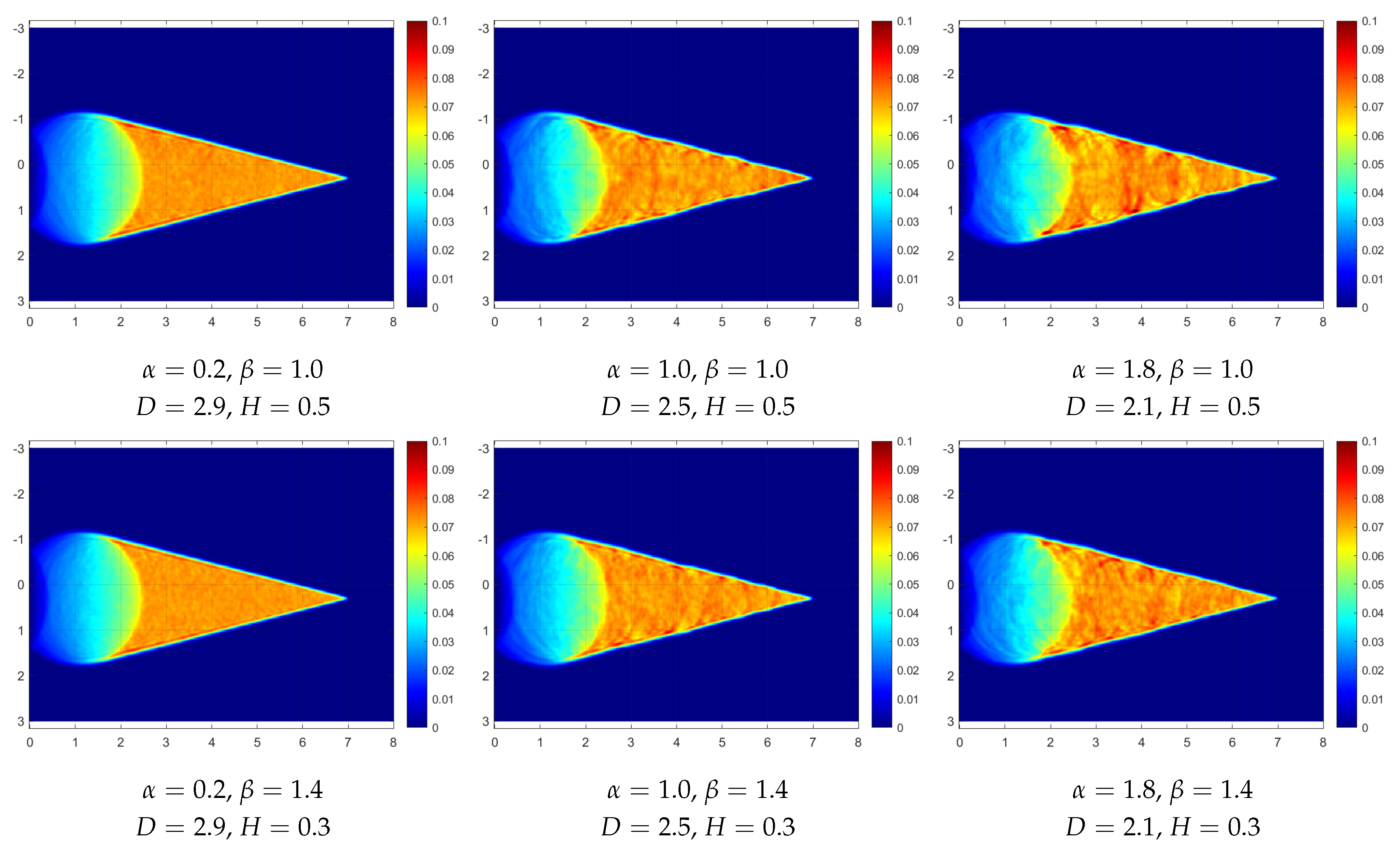
software. The panels of
Figure 4 give such
T fields for
simulated as a Cauchy type RF for a range of
and
coefficients, with the mean
= 4 s and the variance
= 0.4 s (recall Equation (
11)). Similarly, the panels of
Figure 5 give such
T fields for
simulated as a Dagum type RF for a range of
and
coefficients, also for
= 4 s and
= 0.4 s (recall Equation (
12)). In all the cases, the heat source
Q travels on a straight path from the left to the right at a constant speed of
cm/s. Given that
cm/s, the nominal Mach number equals 4. This corresponds to a surgeon’s hand moving four times faster than the speed of second sound in a particular tissue.
The effects of material spatial randomness on the resulting Mach wedges are evident in all the panels and, as expected, they depend on the particular
(or
D) and
(or
H) values (recall (13)). To compare any particular temperature field (
r) resulting from a realization of the random medium with the temperature field obtained on a homogeneous domain (
h), a cross-correlation coefficient (or so-called normalized covariance)
is employed [
17]:
This formula allows a quantitative cross-comparison of two identically sized panels. Thus, both fields,
r and
h, are obtained on rectangular domains of the same size: 438 × 250 = 109,500. The domain was cropped to remove the outer edge (dark blue region in the graphs) where nothing is happening. Thus, the
r field is the set
while the
h field is the set
where
I = 109,500. The cross-correlation coefficients
so calculated are collected for various cases in
Table 1 and
Table 2:
Table 1 shows the cross-correlation coefficients comparing the results from Cauchy RFs with a homogeneous field of
= 4 s.
Table 2 shows the cross-correlation coefficients comparing the results from Dagum RFs with a homogeneous field of
= 4 s.
The effects of changing values of
and
can be observed from
Table 1 and
Table 2; the structure of these tables corresponds to the layout of
Figure 2 and
Figure 3. For Cauchy RFs, smaller
and larger
values result in wedges that are more similar to the homogeneous case. On the other hand, for Dagum RFs, results from larger
and larger
are closer to the homogeneous case, except when
or
is equal to
, where the correlations are high but the effect of changing the other parameter is not obvious from the cross-correlation coefficients.
Overall, even though the correlation numbers are not dramatically different from each other, the effects can actually be observed from the figures and simulation movies. To see the latter, the reader only needs to click on a select panel in
Figure 4 and
Figure 5. From the Cauchy RFs in
Figure 4, we can see that, as the fractal dimension
D (which measures roughness) increases, many small waves generated by the material fluctuations end up smoothing each other out, causing the final result to be closer to the homogeneous case. On the other hand, as the Hurst coefficient
H (describing the long-range memory) decreases below
and as the field gets more anti-persistent, we can see similar effects of smaller fluctuations causing a more homogeneous outcome.
Intuitively, we can see that the waves propagate more homogeneously on fields that are rougher locally on a smaller scale but have weaker fluctuations globally on a larger scale. For the Dagum RFs of
Figure 5, which seem to be rougher overall than the Cauchy RFs, the effect of increasing the fractal dimension
D is the opposite, which might indicate that the added roughness is not local enough.
