Article

A Data-Driven Memory-Dependent Modeling Framework for Anomalous Rheology: Application to Urinary Bladder Tissue

1
Department of Mechanical Engineering & Computational Mathematics, Science and Engineering, Michigan State University, East Lansing, MI 48824, USA
2
Department of Mechanical Engineering, Michigan State University, East Lansing, MI 48824, USA
3
Department of Mechanical Engineering & Statistics and Probability, Michigan State University, East Lansing, MI 48824, USA
*
Author to whom correspondence should be addressed.
Fractal Fract. 2021, 5(4), 223; https://doi.org/10.3390/fractalfract5040223
Submission received: 30 September 2021 / Revised: 27 October 2021 / Accepted: 2 November 2021 / Published: 16 November 2021
(This article belongs to the Special Issue Fractal Media and Fractional Viscoelasticity)

Abstract

:
We introduce a data-driven fractional modeling framework for complex materials, and particularly bio-tissues. From multi-step relaxation experiments of distinct anatomical locations of porcine urinary bladder, we identify an anomalous relaxation character, with two power-law-like behaviors for short/long long times, and nonlinearity for strains greater than 25 % . The first component of our framework is an existence study, to determine admissible fractional viscoelastic models that qualitatively describe linear relaxation. After the linear viscoelastic model is selected, the second stage adds large-strain effects to the framework through a fractional quasi-linear viscoelastic approach for the nonlinear elastic response of the bio-tissue of interest. From single-step relaxation data of the urinary bladder, a fractional Maxwell model captures both short/long-term behaviors with two fractional orders, being the most suitable model for small strains at the first stage. For the second stage, multi-step relaxation data under large strains were employed to calibrate a four-parameter fractional quasi-linear viscoelastic model, that combines a Scott-Blair relaxation function and an exponential instantaneous stress response, to describe the elastin/collagen phases of bladder rheology. Our obtained results demonstrate that the employed fractional quasi-linear model, with a single fractional order in the range α = 0.25–0.30, is suitable for the porcine urinary bladder, producing errors below 2 % without need for recalibration over subsequent applied strains. We conclude that fractional models are attractive tools to capture the bladder tissue behavior under small-to-large strains and multiple time scales, therefore being potential alternatives to describe multiple stages of bladder functionality.

1. Introduction

Bio-tissues are complex and multi-functional materials, optimized for their specific host organisms, and constrained by limited set of building blocks and available resources [1]. While the mechanical behavior of a number of standard engineering materials is quite well-understood, there is still a significant effort towards bio-materials, where microstructure heterogeneities, randomness and small scale physical mechanisms lead to non-standard and at times counter-intuitive responses. Power-law viscoelastic rheology is a complex response observed in many bio-tissues such as arteries [2], cartilage [3], lungs [4], smooth muscle [5], liver and kidneys [6], among other classes of materials. These power-law materials, also termed anomalous, exhibit one or more power-law scalings for creep/relaxation in the form J ( t ) t β and G ( t ) t β across multiple time-scales. Similar anomalous behaviors are also present for dynamic storage/dissipation in the frequency domain [7,8]. The origin of this power-law behavior at the continuum level is linked to (non-Fickian) sub-diffusive processes [9] in the corresponding fractal-like micro-structures [10].
The aforementioned anomalous non-exponential behavior usually requires a significant number of material parameters when employing standard viscoelastic models. These consist of mechanical arrangements of linear springs and Newtonian dashpots, which induces a finite number of relaxation modes, which may lack predictability when performing outside the experimental time scales [3,11]. In this regard, fractional models become attractive alternatives, since their integro-differential operators naturally utilize power-law convolution kernels, coding self-similar microstructural features in a reduced-order mathematical language with smaller parameter spaces. Therefore, they have been employed as compact and predictive models for a number of anomalous systems, such as biological materials [2,3,4,5,6], fluid turbulence [12,13,14], and instabilities [15]. We particularly note that such predictability has been shown to extend across different experiments (relaxation/creep) in certain cases [11]. Additionally, calibrating experimental data with a set of existing rheological models leads to a material model selection problem, which is inherently ill-conditioned, since multiple models can pragmatically yield similar errors when confronted to experiment. In this work, we attempt to reduce this implicit ill-posedness by introducing fractional-order models as attractive alternatives to their integer-order counterparts, and employed to urinary bladder (UB) tissue modeling. Our fractional modeling framework aims to obtain compact mathematical models with a reduced number of material model parameters, while introducing a minimal, but sufficient number of fractional rheological elements that capture the qualitative response of multiple power laws and minimizes the errors, also rigorously taking into account the corresponding power-law memory effects.
The lower urinary tract, and especially the UB, is a highly dynamic organ system. To ensure its proper function, the bladder needs to be able to significantly increase in size while maintaining a low internal pressure, and this ability is dictated by the mechanics of the bladder wall. Specifically, during filling, the bladder tissue must leverage its viscoelastic characteristics to accommodate for large deformations without resulting in significant increase of luminal pressure. When this behavior is compromised due to disease, the resulting increase in pressure might generate a high-pressure urine reflux from the bladder to the kidneys, resulting in renal failure [16,17]. To increase the complexity of the organ mechanics, the characteristics of the bladder differ between different anatomical locations (i.e., dorsal, ventral, lateral, lower-body, trigone) [18,19] and orientations (i.e., longitudinal/apex-to-base and circumferential/transverse) [18,19,20,21,22,23,24,25,26]. To describe the behavior of bladder tissue, both hyperelastic and viscoelastic models have been used in the literature. Hyperelastic models have included continuum-based Ogden [26], exponential [21,22,27,28], and fiber recruitment [25] models, as well as fluid pressure-based models assuming the bladder in spheroidal shapes [26,29,30,31,32,33]. Viscoelastic models have included various forms of spring-dashpot [23,34,35,36,37,38,39,40,41,42,43,44,45] and quasi-linear viscoelastic [24,46,47] models. However, due to the differences in mechanical testing protocols as well as modeling, most of the results cannot be compared with one another and often results in contradicting conclusions. While several pathologies of the lower urinary tract are associated with dramatic changes of the mechanical behavior of the bladder wall [48], still much is unknown about the mechanisms that affect this organ, not just in diseased states but in healthy as well. In this study, we focus on the healthy behavior of the porcine urinary bladder, which a present work suggested is a good model for the human urinary bladder.
Although fractional linear viscoelasticity has been succesfully employed in a number of biomechanical applications, additional modeling considerations are necessary when dealing with other material nonlinearities, such as large strains. This would imply that the material relaxation behavior depends on both time and applied strains, which requires additional modeling considerations. In the UB case, Korossis et al. [18] reports the small-strain regime to be drive by elastin, while a stiffer response for large strains was driven by collagen. Jokandan et al. [49] characterized the quasi-static stress-strain response of the UB as exponential-like. To address such behavior, a practical and well-known class of models is the quasi-linear-viscoelastic (QLV) theory by Fung [50], which considers a multiplicative coupling between a linear viscoelastic relaxation and a nonlinear elasticity term. While the original formulation utilizes a finite spectrum of relaxation times, fractional extensions of the QLV theory have been developed and employed for the response of bio-tissues [2,51]. Doehring et al. [51] employed a Mittag-Leffler-type reduced relaxation function that captured the short and long term behaviors of aortic valve cusp [51]. Craiem et al. [2] developed a fractional Kelvin-Voigt-type reduced relaxation function with an exponential instantaneous response, which was successfully applied to the nonlinear viscoelasticity of arterial walls. Regarding the nonlinear viscoelastic modeling of the UB, Natali et al. [24], developed an anisotropic, visco-hyperelastic model, which was validated through a uniaxial experiment under cyclic loads. Nagatomi et al. [46] studied the nonlinear behavior of rat bladders, by calibrating a two-dimensional QLV model to bi-axial relaxation data from bladders of subjects that were healthy and with spinal cord injury. Their findings reported a need for new models to account for both normal and pathological states, due to tissue remodeling.
To the authors’ best understanding, although existing studies have addressed the nonlinear viscoelastic of the UB for different subjects and loading conditions, there are no studies in the literature leveraging the use of fractional viscoelastic models to model potential, emerging power-law behaviors. In this work we develop a data-driven fractional modeling framework for linear and quasi-linear viscoelasticity to account for both anomalous power-law relaxation and large strains of bio-tissues. We validate the developed framework for the first time in the uniaxial relaxation of porcine urinary bladder tissue for a wide range of applied strains. The characteristics of our experimental procedure are:
  • We obtain the porcine UB uniaxial relaxation data from small-to-large strains of five distinct anatomical locations.
  • Our relaxation experiments are performed under increasingly larger strains, without intermediate unloading steps or tissue preconditioning.
  • The mechanical response of the UB indicates nonlinear viscoelastic behavior with power-law relaxation, characterizing an anomalous, non-exponential behavior.
Given the anomalous nonlinear response of the UB tissue, we develop our two-stage anomalous modeling framework as follows:
  • In the first stage, we develop an existence study that considers a set of linear fractional building block models (Scott-Blair, fractional Kelvin-Voigt, fractional Maxwell), which are selected according to the multi-power-law nature of the relaxation data and calibration errors at the linear viscoelastic regime.
  • In the second stage, we account for the large strain behavior of the corresponding tissue, by employing a fractional quasi-linear viscoelastic (FQLV). The goal is to extend the quality of power-law relaxation (due to the material’s fractal microstructure) to the large strain regime of the tissue of interest.
We employed the aforementioned two-stage formulation to the UB experimental data, and obtained the following main findings;
  • All candidate fractional linear viscoelastic models provide sufficiently accurate fits for single-relaxation steps under smaller strain levels, where the two fractional order Maxwell model is the most suited for the UB data.
  • The employed four-parameter FQLV model with a reduced Scott-Blair relaxation function and exponential instantaneous stress response was successful over five consecutive relaxation steps, with root mean squared errors below 2 % , and without the need of model recalibration between applied step strains.
  • The lower-range of obtained fractional orders is around α = 0.17–0.30, which is compatible with the observed long-time slopes of the UB relaxation data. Small α values have been suggested to indicate strong fractality in bio-tissue microstructures such as collagen fibers [51].
The rest of the paper is organized as follows. In Section 2 we present the problem setup and methodology, with the uniaxial UB stress relaxation experiments and our proposed fractional modeling framework for biotissues, comprised of linear and quasi-linear fractional models. In Section 3, we present our obtained linear viscoelasticity results for the UB relaxation under the first strain step, and the fractional quasi-linear viscoelastic model for all consecutive strain steps, followed by the discussions and potential improvements of the work. Finally, in Section 4, we provide the concluding remarks of this work and future directions.

2. Problem Setup and Methodology

2.1. Urinary Bladder Experimental Relaxation Tests

Five samples from a single porcine UB were extracted from distinct anatomical locations as shown in Figure 1a. The locations are given and denoted by: Dorsal (D), lateral (L), lower body (LB), trigone (T), and ventral (V). The samples were extracted with a 1 cm × 3 cm leather punch in the apex-to-base direction as shown in Figure 1b. Each sample was clamped, as illustrated in Figure 1c,d, and subjected to five consecutive stress relaxation stages, under prescribed step strains ε i = 0.25 , 0.50 , 1.00 , 1.50 , 2.00 over 30, 45, 45, 45, and 45 min, respectively. Besides the strain inputs, the force denoted by F data ( t ) is measured by a 10 [ l b ] load cell throughout the duration of the test. The cross-sectional area A data ( t ) of each sample is calculated by taking top and side view pictures that are converted to binary images which are processed in MATLAB®, respectively estimating the base b ( t ) and height h ( t ) dimensions of the samples after the application of each consecutive step strain ε i . The updated cross-sectional area is assumed to remain constant throughout the relaxation at each strain level, and is evaluated as A data = b ( t ) h ( t ) . Given force and area time-series, the true stress is evaluated as σ data ( t ) = F data ( t ) / A data ( t ) .
Once the stress σ data ( t ) and strain ε data ( t ) time-series are obtained, we filter the data through a moving average filter with a time-window of thirty neighbor data points. Figure 2 illustrates the relaxation curves for all samples in linear and log-log scales. We observe a characteristic power-law scaling for long-time behavior, which is evident in Figure 2b. As will be shown later through fractional model fits, the relatively low scaling coefficient β indicates an anomalous behavior of predominantly elastic nature, with a plateau with low decay rates σ t β at larger time-scales (i.e., t > 400 [ s ] ). We also note that the trigone and lower body specimens yielded higher stress levels, particularly at very high strains, while the dorsal specimen yielded lower overall values. This is in accordance to stress-strain results obtained by Korossis et al. [18], that indicated statistically significant, higher collagen phase slopes for the lower body and trigone regions.
We analyze the presence of strain dependency on the UB relaxation behavior, in order to determine if the viscoelasticity is of linear or nonlinear nature. Therefore, we employ the definition of linear relaxation modulus G ( t ) [ Pa ] , applied for each fixed strain application from experimental data [52]:
G data ( t ) : = σ data ( t ) / ε i ,
with i = 0 , 1 , , N steps . In addition to the strain dependency on the relaxation behavior, the above definition also allows us to identify the presence of additional power-laws or stretched exponential behaviors in the tissue response. Figure 3 illustrates the obtained relaxation moduli for all UB samples and relaxation steps, after employing (1) into the stress time-series data of Figure 1 and performing a translation to a reference initial time, here taken as the first time-step of the data. We observe that although the relaxation moduli data for each sample is almost linear for ε i = 0.25 , 0.50 , since the curves approximately overlap (except for the trigone sample), the behavior of G data is clearly time- and strain-dependent. Furthermore, the degree of nonlinearity is more pronounced for the lower body and trigone samples, and less pronounced for the dorsal sample. Interestingly, we notice two limiting power-law behaviors for short and long times. The short time behavior appears to have a stretched exponential nature, with a limiting power law of smaller magnitude β 1 , while the long time behavior is associated with a power-law of larger magnitude β 2 , see Figure 3f. Nevertheless, the relaxation behavior clearly transitions from a slower regime to a faster regime, even though the latter still presents a far-from-equilibrum response (no equilibrium glass state) within the experimental time scales. Larger standard deviations for the long time power-law were observed for the trigone region due to its distinct response for ε 0 = 0.25 . We remark that this analysis is just performed to infer the nonlinear relaxation quality the data, and we do not intend to construct a master curve for each UB sample.

2.2. A Fractional Viscoelastic Modeling Framework for Anomalous Tissue Rheology

We develop a two-stage framework to assess the qualitative linear/nonlinear relaxation behavior of anomalous materials and identify the most feasible fractional viscoelastic models, in order to alleviate the inherent ill-posedness of model selection problems. In the first stage, we develop an existence study to identify the admissible set of anomalous constitutive laws that satisfy the quality of the experimental linear relaxation behavior, while shedding light on the corresponding microstructural constituents associated to anomalous behavior. In the second stage, we incorporate large strain effects to the relaxation quality, based on the nonlinear nature of the tissue of interest.

2.2.1. First Stage: An Existence Study of Fractional Linear Viscoelastic Models

Starting with the Scott-Blair (SB) model as the fundamental building block, we construct building block models through parallel and serial combinations to obtain the fractional Kelvin-Voigt (FKV) and fractional Maxwell (FM) models. In our approach, we take into account the anomalous qualities present in the experimental relaxation data and compare them with each of the candidate building block models. Each of the models exhibit distinguished material complexities, such as distinct asymptotic behaviors of relaxation G ( t ) , multiple power-law regimes, slower/faster relaxation at the asymptotic stages [53,54] and presence of material nonlinearities. In the last part of the existence study we classify the candidate models according to their anomalous response, which together with obtained fitting errors and number of material parameters, constitutie the criteria for the model selection procedure. Given the experimental data presented in Section 2.1, we focus on the first relaxation step ( ε 0 = 0.25 ) of Figure 2 and Figure 3 for the first stage of our data-driven framework. Our objective is to demonstrate how fractional viscoelastic models are able to capture the UB relaxation with simplistic mechanical arrangements and a small number of material parameters.
The rheological building block for our framework is the fractional SB viscoelastic element, which compactly represents an anomalous viscoelastic constitutive law connecting the stresses and strains:
σ ( t ) = E 0 C D t α ε ( t ) ,
with t > 0 , ε ( 0 ) = 0 , and constant fractional order in the range 0 < α < 1 , which provides a material interpolation between Hookean ( α 0 ) and Newtonian ( α 1 ) elements. The operator 0 C D t α ( · ) represents the time-fractional Caputo derivative given by:
0 C D t α u ( t ) : = 1 Γ ( 1 α ) 0 t u ˙ ( s ) ( t s ) α d s ,
where Γ ( · ) represents the Euler-gamma function [54] and u ˙ = d u / d t . The pair ( α , E ) uniquely represents the SB constants, where the pseudo-constant E [ Pa . s α ] compactly describes textural properties, such as the firmness of the material [11,55]. In this sense E is interpreted as describing a snapshot of a non-equilibrium dynamic process instead of an equilibrium state. The corresponding rheological symbol for the SB model represents a fractal-like arrangement of springs and dashpots [7,56], which we interpret as a compact, upscaled representation of a fractal-like microstructure. Regarding the thermodynamic admissibility of the SB element and more complex models (i.e., plasticity and damage) involving it, we refer the reader to Lion [57] for the SB model, and Suzuki et al. [58]. The relaxation function G SB ( t ) [ Pa ] for the SB model is given by the following single, inverse power-law form:
G SB ( t ) : = E Γ ( 1 α ) t α ,
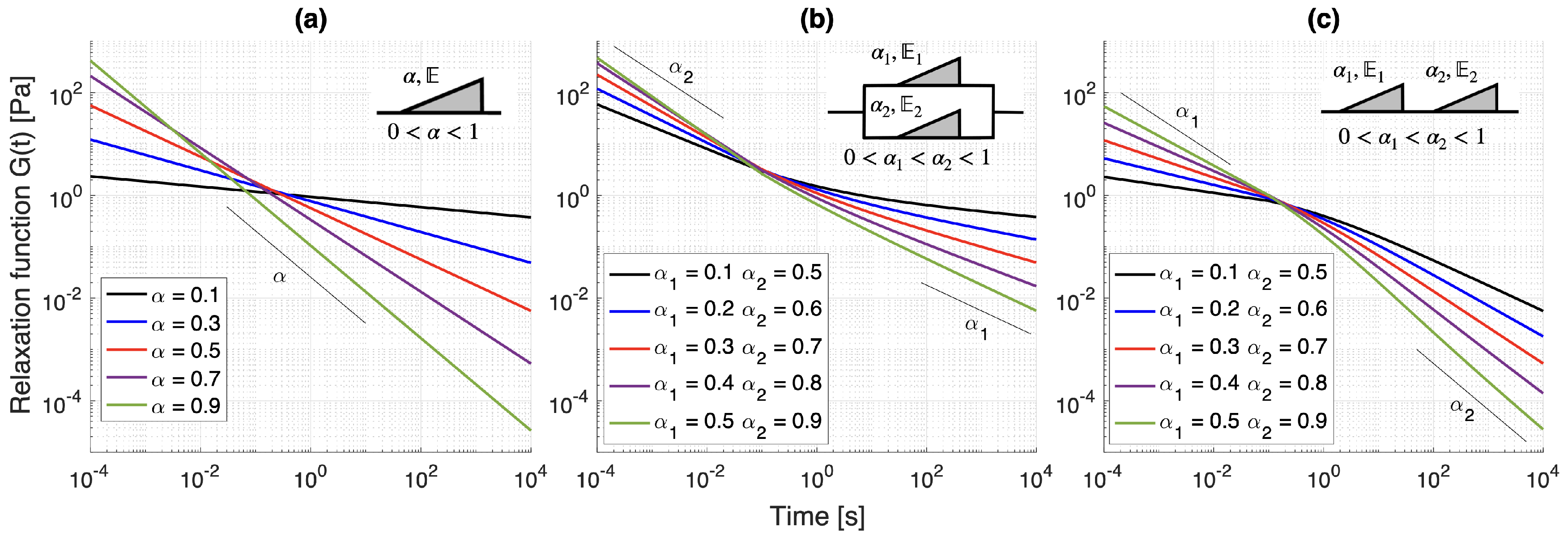
which is the convolution kernel of the integro-differential form in (3), with a modulating pseudo-constant E for fixed α . Figure 4a illustrates the behavior of G SB ( t ) , which is scale-free, i.e., a single power-law is present for all t > 0 . We note that although this relaxation response may seem to be oversimplified, it provides a flexible constitutive interpolation able to, at the very least, take into account the long-term anomalous dynamics of materials, such as the power-law β 2 in Figure 3. This also allows the SB element to capture, in certain time-scales, power-law behaviors induced by predominantly elastic microstructures, such as collagen networks [51] with small α -values. We also note that single collagen fibril relaxation data [59] has been calibrated to single-order fractional Kelvin-Zener models (where a single SB element is combined with Hookean springs), with reported values in the range α = 0.12–0.21 [60]. Similarly, the macroscopic response of ultrasoft tissues such as the brain, which has a more fluid-like character with significant microscopic inter-cell body displacements in the deformation process [61], has also been captured using SB elements combined with Hookean springs [62,63]. Kohandel et al. [62] calibrated a single-order dynamic modulus of a fractional Kelvin-Zener model to bovine brain tissue, obtaining a fractional order α = 0.6 . Through relaxation experiments, Stamenović et al. [63] calibrated a similar model to bovine brain paerenchima also reporting a high value of α = 0.64 .
We utilize the SB model as our rheological building block, and define a set of “building block models”, which introduce a higher degree of material complexity through multiple power-law behaviors for relaxation and therefore distinct anomalous regimes for small and large time-scales. This multi-fractal type of rheology is characteristic of cells [63] and biological tissues [64], due to their complex, hierarchical and heterogeneous microstructure. Here we consider the two simplest canonical combinations of SB elements. Through a parallel combination, we obtain the fractional Kelvin-Voigt (FKV) model, which has the following stress-strain relationship [56]:
σ ( t ) = E 1 0 C D t α 1 ε ( t ) + E 2 0 C D t α 2 ε ( t ) ,
with t > 0 , ε ( 0 ) = 0 , fractional orders 0 < α 1 , α 2 < 1 and associated pseudo-constants E 1 [ Pa . s α 1 ] and E 2 [ Pa . s α 2 ] . The corresponding relaxation modulus G ( t ) , is also an additive form of relaxation involving two SB elements:
G FKV ( t ) : = E 1 Γ ( 1 α 1 ) t α 1 + E 2 Γ ( 1 α 2 ) t α 2 .
Figure 4b illustrates the relaxation function G FKV for several fractional order values. We notice a response characterized by two power-law regimes, with a transition from faster to slower relaxation slopes. The asymptotic responses for small and large time-scales are given by G FKV t α 2 as t 0 and G FKV t α 1 as t . We note that this quality allows the FKV model to describe materials that reach an equilibrium behavior for large times when α 1 0 , which is intuitive from the mechanistic standpoint as one of the SB elements becomes a Hookean spring. Regarding applications of the FKV model to bio-tissue constituents, Bonfanti et al. [60] has found the combination of low-high fractional orders to be proper for bovine trachea smooth muscle cells, recovering α 1 = 0.1 and α 2 = 0.78 .
Finally, through a serial combination of SB elements, we obtain the fractional Maxwell (FM) model [11], given by:
σ ( t ) + E 2 E 1 0 C D t α 2 α 1 σ ( t ) = E 2 0 C D t α 2 ε ( t ) ,
with t > 0 , fractional orders 0 < α 1 < α 2 < 1 , the additional constraint 0 < α 2 α 1 < 1 , and two sets of initial conditions for strains ε ( 0 ) = 0 , and stresses σ ( 0 ) = 0 . We note that in the case of non-homogeneous ICs, one requires compatibility conditions [54] between stresses and strains at t = 0 . The corresponding relaxation function for this building block model assumes a more complex, Miller-Ross form [11]:
G FM ( t ) : = E 1 t α 1 E α 2 α 1 , 1 α 1 E 1 E 2 t α 2 α 1 ,
where E a , b ( z ) denotes the two-parameter Mittag-Leffler function, defined as [54]:
E a , b ( z ) = k = 0 z k Γ ( a k + b ) , R e ( a ) > 0 , b C , z C .
Interestingly, the presence of a Mittag-Leffler function in (8) leads to a stretched exponential relaxation for smaller times and a power-law behavior for longer times, as illustrated in Figure 4. We also observe that the limit cases are given by G FM t α 1 as t 0 and G FM t α 2 as t , indicating that the FM model provides a behavior transitioning from slower-to-faster relaxation. Furthermore, when α 2 1 , the FM model presents a fluid-like behavior for long times [53], and therefore allowing a fast relaxation, similar to its integer-order counterpart. We refer the reader to the recent work by Bonfanti et al. [60] for a number of applications of the aforementioned models. We notice that both FKV and FM models are able to recover the SB element with a convenient set of pseudo-constants. Furthermore, we also outline more complex building block models that yield more flexible responses, including three to four fractional orders, such as the fractional Kelvin-Zener (FKZ), fractional Poynting-Thomson (FPT), and fractional Burgers (FB), which in turn are able to recover the FKV and FM models. We refer the reader to the works [56,60] for more details on such models.

2.2.2. Second Stage: Fractional Quasi-Linear Viscoelastic Modeling

The presented models in Section 2.2.1 provide candidates for power-law relaxation functions that describe the anomalous linear viscoelasticity of biotissues, however, in such materials the stress-strain relationship may becomes nonlinear as fibers in collagen networks transition from entangled to aligned with the applied load direction. Therefore, the viscoelastic behavior itself becomes nonlinear and the relaxation function has an intrinsic dependency on the strain levels, as observed in Figure 3 under successive large step-strain applications. To incorporate this additional effect to our modeling framework, we follow [2,50], and employ the following quasi-linear, fractional viscoelastic model (FQLV):
σ ( t , ε ) = 0 t G ( t s ) σ e ( ε ) ε ε ˙ d s ,
where the convolution kernel is given by a multiplicative decomposition of a reduced relaxation function G ( t ) which may be selected from the first stage of the framework, and an instantaneous, nonlinear elastic tangent response with stress σ e . In the work by Craiem et al. [2], the reduced relaxation function has a fractional Kelvin-Voigt-like form with one of the SB elements replaced with a Hookean element. Here, we assume a simpler rheology and adopt a Scott-Blair-like reduced relaxation in the form:
G ( t ) = E t α / Γ ( 1 α ) ,
with the pseudo-constant E with units [ s α ] , since the elastic strains σ e ( ε ) have units of [ Pa ] . We adopt the same, two-parameter, exponential nonlinear elastic part as in [2]:
σ e ( ε ) = A e B ε 1 ,
with A having units of [ Pa ] and B being a non-dimensional tuning parameter for the degree of nonlinearity induced by applied strains. Substituting Equations (11) and (12) into Equation (10), we obtain:
σ ( t , ε ) = E A B Γ ( 1 α ) 0 t e B ε ( s ) ε ˙ ( s ) ( t s ) α d s ,
which differs slightly from the linear SB model (2) in the sense that an additional exponential factor multiplies the function being convoluted. We remark that reduced relaxation forms for the FKV and FM can also be employed in the FQLV framework. For the FKV model, it would lead to a multi-term convolution of the same nature as (13) with fractional orders α 1 and α 2 . Therefore, the same numerical methods employed in Section 2.2.3 could be employed. However, when dealing with a FM reduced relaxation function, a specialized type of quadrature for a Miller-Ross-type of kernel as (8) would be required, potentially with impractical computations of Mittag-Leffler functions for a large number of time-steps.

2.2.3. Numerical Discretizations

We discretize the fractional Caputo derivatives in Equations (2)–(7) through an implicit L1 finite-difference scheme [65]. Therefore, we consider a uniform time-grid with N time-steps of size Δ t , such that t n = n Δ t , with n = 0 , 1 , , N . We remark that although the equations for each of the building block models could be discretized utilizing fast schemes and approaches that treat initial time singularities (see [66,67] and references therein), the number of utilized data-points is not large, with N d a t a 3000 for the first relaxation and N d a t a 25,000 for all steps. Also, we avoid the singularity nearby t 0 since the first relaxation step is applied at approximately 80 s. Nevertheless, the non-smooth nature of the loading would degenerate most of the existing numerical methods for FDEs, and we found that the employed method in this work with the Δ t described in Section 3 is sufficient for the accuracy to reach the plateau of the experimental data, such that model error is dominant.
In the following, we present the discretized forms for each of our employed linear fractional viscoelastic models. We start with the stresses for the SB model evaluated at t = t n + 1 :
σ n + 1 = C 1 ε n + 1 ε n + H α 1 ε ,
with discretization constant C 1 = E / ( Γ ( 2 α ) Δ t α ) .
For the FKV model, we obtain:
σ n + 1 = C 1 ε n + 1 ε n + H α 1 ε + C 2 ε n + 1 ε n + H α 2 ε ,
with discretization constants C 1 = E 1 / ( Γ ( 2 α 1 ) Δ t α 1 ) and C 2 = E 2 / ( Γ ( 2 α 2 ) Δ t α 2 ) .
Finally, for the FM model, we have:
σ n + 1 = C 1 ε n + 1 ε n + H α 1 ε + C 2 σ n H α 1 α 2 σ 1 + C 2 ,
with discretization constants C 1 = E 1 / ( Γ ( 2 α 1 ) Δ t α 1 ) and C 2 = ( E 1 / E 2 ) / ( Γ ( 2 α 1 + α 2 ) Δ t α 1 α 2 ) . The history terms H ν u with fractional order ν in the above equations are given by the following form:
H ν u = j = 1 n b j u n + 1 j u n j ,
with weights b j ν : = ( j + 1 ) 1 ν j 1 ν .
The discretization for the FQLV model (13) employed in this work is shown in [68], which is a straightforward, fully-implicit, L1 finite-difference approach with a trapezoidal rule employed on the additional exponential factor. Therefore, the discretized stresses for the FQLV model are given by:
σ n + 1 = C 1 exp ( B ε n + 1 2 ) ε n + 1 ε n + H α ε , σ e ε ,
with constant C 1 = E A B / ( Δ t α Γ ( 2 α ) ) . The discretized history load in this case is given by:
H α ε , σ e ε = k = 1 n exp ( B ε n k + 1 2 ) ε n k + 1 ε n k b k ,
with discretization weights b k α = ( k + 1 ) 1 α k 1 α and ε i + 1 2 = ( ε i + ε i + 1 ) / 2 . The presented discretization has an accuracy of O ( Δ t 2 α ) , and we refer the reader to [68] for simulations of numerical convergence.

2.3. Model Optimization

We perform the model fits through a particle-swarm optimization (PSO) algorithm [69], which was implemented in MATLAB. The adopted PSO parameters are a population N p o p = 30 and N i t = 1000 iterations for the linear cases and N i t = 100 iterations for the nonlinear cases. For the linear viscoelastic fits, we set the initial material pseudo-parameter in the 0 E 10 8 [Pa.s α ], and the fractional orders are constrained in the 0.0001 α 0.9999 range, to ensure that the employed fractional models are able to recover simpler fractional counterparts and also standard rheological elements, if required by the experimental data. For nonlinear cases, we estimate ranges for parameters A and B of the FQLV model by fitting the instantaneous stress response (12) to each stress peak in every step-strain application of Figure 2. From this preliminary estimate, we have obtained parameters in the ranges 10 4 A 10 5 [Pa] and 0 B 2 , which are taken as input parameter ranges for the PSO algorithm. For the relaxation parameters of the FQLV, as in [2], we note that the nature of the power-law relaxation kernel, it is nontrivial to obtain a normalized G ( 0 + ) = 1 . Nevertheless, for the pseudo-constant we set the range 0 E 1 and for the fractional order α we employ the same range as the linear case.
Since the stresses σ d a t a ( i ) and strains ε d a t a ( i ) from the relaxation dataset are non-uniform in time, we perform a linear (first-order accurate) interpolation of the strains ε d a t a ( i ) to an uniform grid. We then utilize the input strains and compute the global best solution for stress for every PSO iteration through (14), (15), (16), or (17). Then, we linearly interpolate the stress back to the nonuniform grid to obtain σ m o d e l . The time-step size for the uniform grid solution is set to Δ t = 0.495 [s], which is the minimum time interval between two consecutive data-points. For verification purposes, we tested smaller step-sizes ( Δ t = 0.0495 ) and did not obtain improved results, and we note that all employed numerical discretizations for fractional models are fully-implicit. Therefore, our verification step indicates that model error dominates over discretization error for the employed time-step size. The cost function is defined as:
C o s t : = i = 0 N d a t a σ i d a t a σ i m o d e l 2 .
The adopted error measures in this work are the normalized least-squares error (LSE) and root mean squared error (RMSE) between the experimental and mapped simulated stresses, which are respectively given by:
L S E : = i = 1 N d a t a σ i d a t a σ i m o d e l 2 i = 1 N d a t a σ i d a t a 2 × 100 % , R M S E : = 1 max ( σ d a t a ) i = 1 N d a t a σ i d a t a σ i m o d e l 2 N d a t a × 100 % .
Finally, all numerical simulations were run in a computer system with Intel Xeon Gold 6148 CPUs with 2.40 GHz.

3. Results and Discussion

3.1. Linear Viscoelasticity

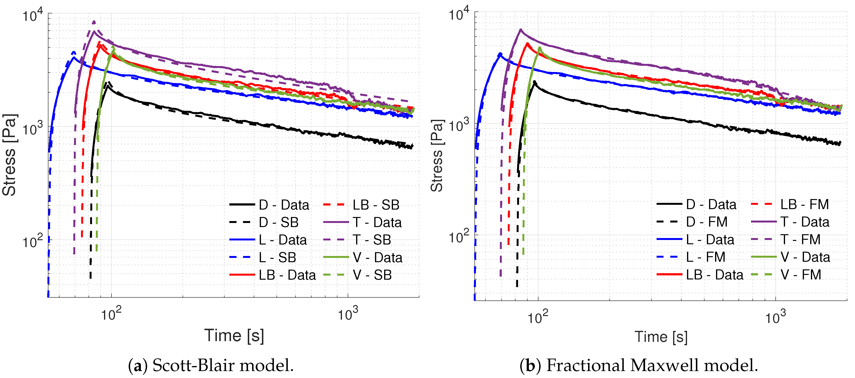
Figure 5 illustrates the obtained fits for all bladder samples utilizing an SB model, for the first strain step ( ε 0 = 0.25 ) . We observe very good fits for most samples, especially at larger time scales, with an exception for the trigone (T) sample due to a sudden stress drop in the experimental data. The fitting quality decreases for all samples at the early relaxation dynamics (nearby the step-strain application), with the SB model underestimating the maximum values of stress peaks. The obtained fractional orders lie in the 0.2–0.3 range (see Table 1), which are similar to the observed long-term power law from the estimated experimental relaxation functions in Figure 3. Furthermore, the least-squared errors lie in the 2–11% range, while the RMS errors are within the 2–4% range. The higher values of the pseudo-constant and fractional order for the trigone sample are likely due to the SB model accounting for both instantaneous and long-term response over its limited set of two parameters. We also note that the FKV model pragmatically recovered the SB model in all instances, where the PSO algorithm obtained optimal values for the fractional orders that are close to the SB model. In addition, the optimal values for one pseudo-constant is either set to zero, or the summation of E 1 and E 2 recovers the value of E for the SB model. This indicates the a FKV model does not improve the bladder fit quality, and one would rather employ a SB model with half the amount of material parameters under the same error levels.
Figure 5 illustrates the obtained fits for the FM model, where the added flexibility of the underlying power-law/Mittag-Leffler relaxation response improves the fitting quality for both short and long time-scales, yielding least squares errors as low as 2.08 % . The obtained parameters in Table 1 indicate the presence of a predominantly elastic power-law α 1 in the 0.17–0.19 range, and a predominantly viscous α 2 in the 0.74–0.99 range. Particularly, the FM model fit for the trigone specimen indicates the recovery of a dashpot element, and thus the corresponding SB element could be replace by a Newton element. Regarding pseudo-constant values, we note that E 1 values have variations that qualitatively agree with the intensity of stress peaks, but E 2 values can vary in several orders of magnitude, which could be due to the presence of multiple local minima or the discrepancy between obtained fractional orders α 2 . In general, the dorsal and ventral samples seem to be the most anomalous, as they present both fractional order values sufficiently far from standard elements.
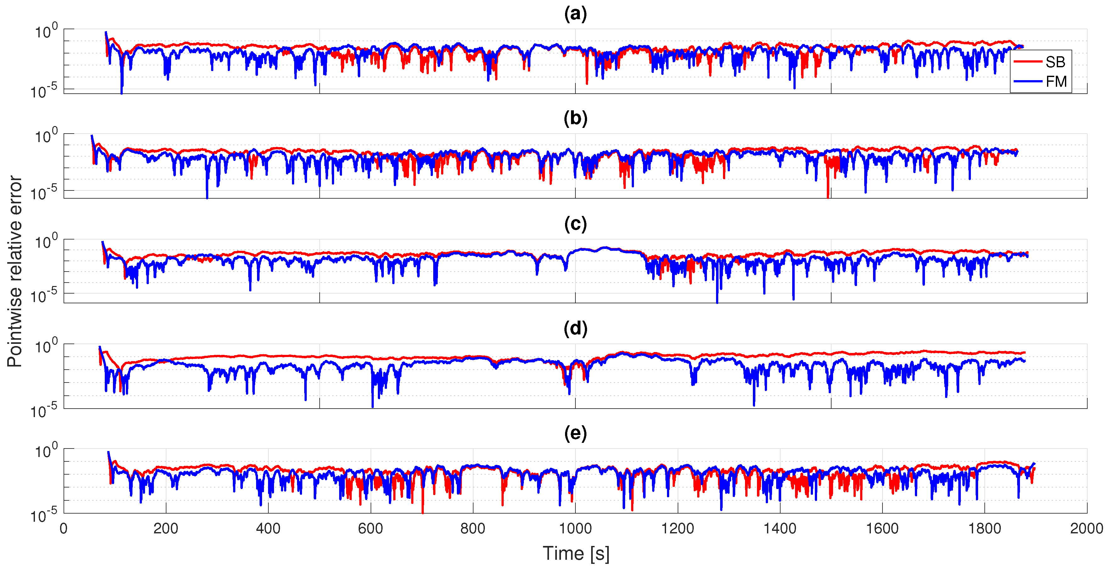
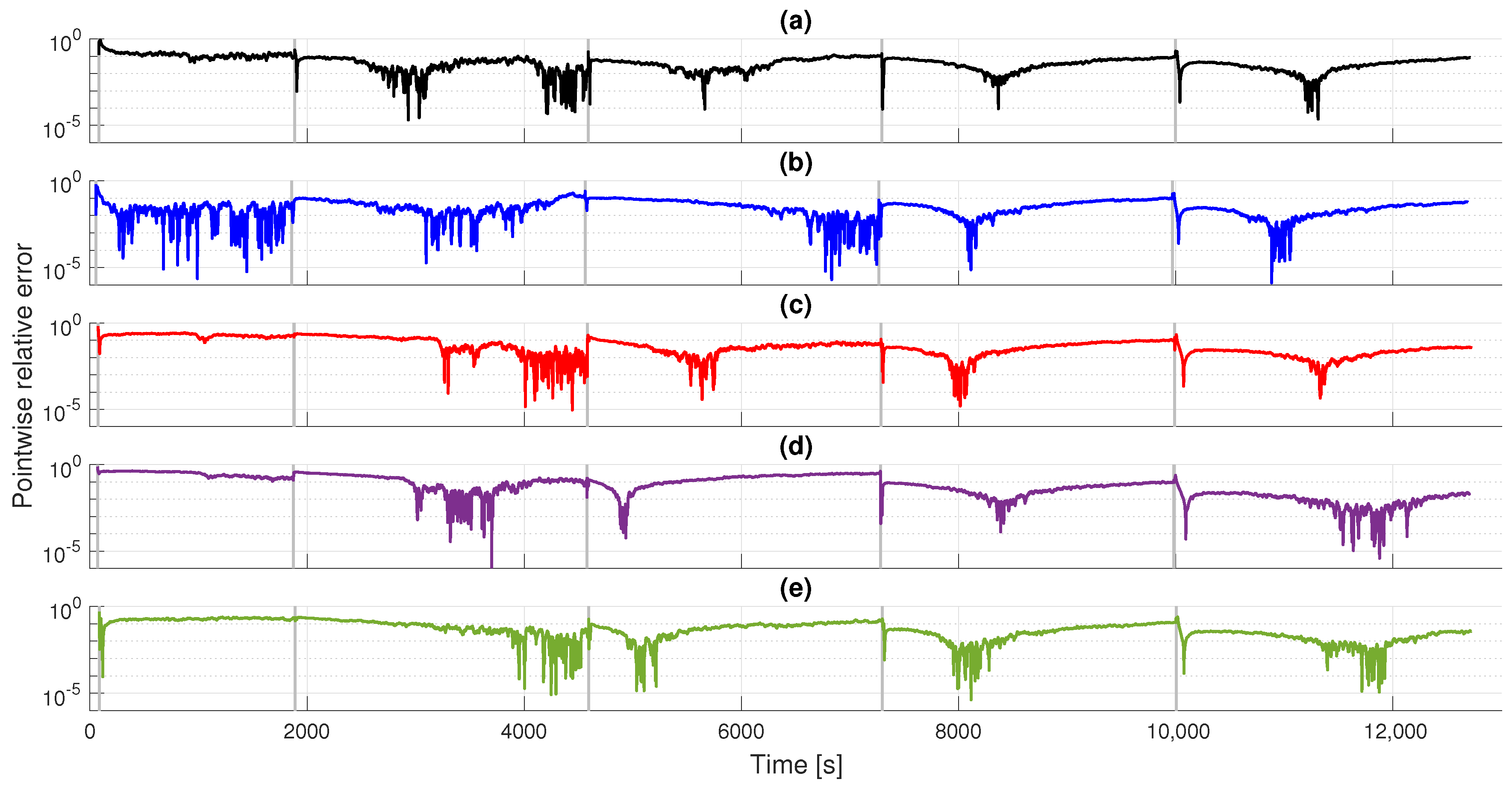
Figure 6 illustrates the pointwise relative errors between the SB and FM models and the experimental data for the first strain step. We notice that the SB element has similar errors as the FM model in the 800 < t < 1200 [s] range and larger errors for longer times for most samples. For shorter time ranges, the SB model has larger errors (up to 1 order of magnitude) for all samples. This reinforces the fact that the FM model is more descriptive of both early and long-term dynamics of bladder relaxation, as the qualitative analysis and estimated experimental relaxation moduli suggest. Furthermore, we also note that the better performance of the FM model is also attributed to better approximating the loading ramp and the peak stress preceding the relaxation behavior.
We also employed more complex fractional linear viscoelastic models, such as fractional Kelvin-Zener, Poynting-Thomson and Burgers’ (see [68] for the models and their corresponding discretizations ). From our employed fitting procedure, all models either recovered or had the same performance as the FM model.

3.2. Nonlinear Viscoelasticity

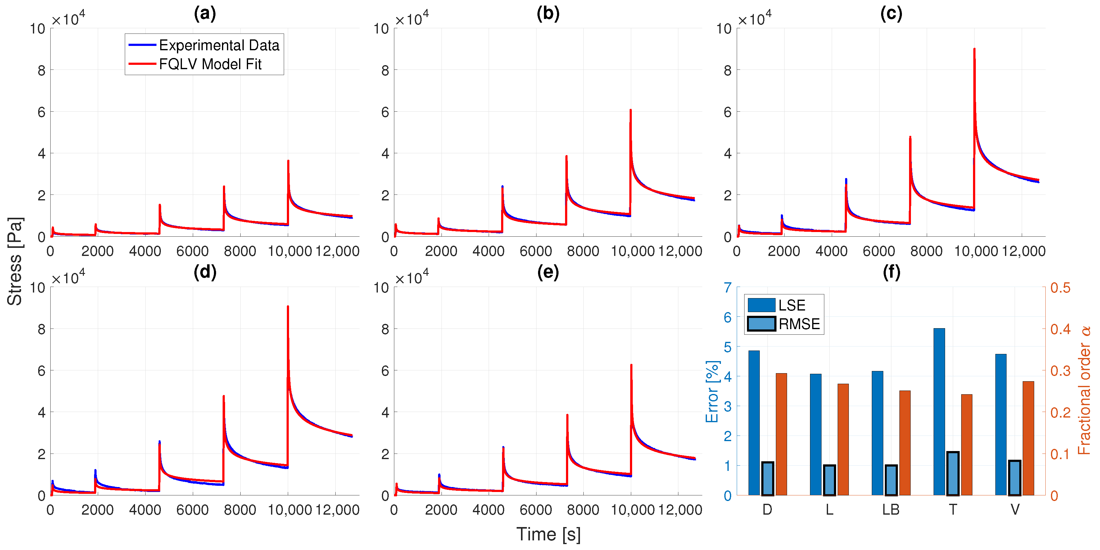
Figure 7 illustrates the obtained fits for the fractional QLV model under all consecutive strain steps, where we observe a very good agreement with the experimental data. Except for the trigone sample, all cases had higher deviations towards the final strain steps. Nevertheless, we note that the error levels are below 6 % (LSE) and 2 % (RMSE) for the entire dataset, under 4 material parameters, which are listed in Table 2. Furthermore, the obtained fractional-orders lie in the range 0.24–0.3 which are in accordance with the estimated power-laws in our a-priori analysis presented in Figure 3. Particularly, the lowest fractional order was obtained for the trigone specimen, and highest for the dorsal one. A slightly higher degree of nonlinearity is also recovered for the trigone and lower-body samples due to the larger values of B.
Finally, Figure 8 illustrates the pointwise relative errors for the FQLV model under all bladder samples and strain steps. We observe a similar error behavior as the SB model in Figure 6, particularly for larger applied strains.

3.3. Discussion

To our best understanding, this was the first work in the literature addressing fractional viscoelastic modeling to bladder tissues. From the results obtained for our building block models, the overall lower range of fractional orders obtained for all linear/nonlinear models is 0.17–0.3, indicating a predominantly elastic yet highly anomalous behavior with smaller decay rates at long times, i.e., the presence of far-from-equilibrium dynamics. A similar parametric range was obtained in other anomalous systems such as arterial wall relaxation [2], aortic valve tissue [51], 1D and 3D brain artery walls under fluid-structure interactions [70,71], canine and bovine liver tissue [72,73], and lung tissue [4]. As suggested by Doehring et al. [51], small α -values can be indications of strong fractality in bio-tissue microstructure such as collagen fibers, which are vastly present in the UB, and particularly with a larger network in the trigone region. The larger values of fractional orders α 2 in the 0.74–0.99 range obtained by the fractional Maxwell model is similar to those obtained for brain tissue relaxation [74] and human ear [75,76]. This indicates a significantly more dissipative behavior, possibly compensating the highly-anomalous behavior provided by the smaller fractional order α 1 for short time-scales, and thus better fitting the slower relaxation nearby the load application. The transitional behavior from slower-to-faster relaxation slopes observed from the UB specimens and captured by the FM model were also noticed in bio-tissues composed of weakly cross-linked collagen networks [64]. We note that although the captured fractional orders α 1 , α 2 for the FM model on the UB relaxation do not quantitatively match the slopes β 1 , β 2 for G d a t a ( t ) in Figure 3, these fractional orders refer to the asymptotic behaviors at t 0 and t , as illustrated in our existence study in Figure 4, and it is likely that relaxation experiments under a larger range of time-scales would yield a better quantitative agreement. For the purpose of our existence study, we consider a qualitative agreement and small error levels to be sufficient to select a valid candidate building block model.
The nonlinear viscoelastic behavior was well approximated by the employed FQLV model, which decomposes the relaxation kernel in a multiplicative fashion into a power-law reduced relaxation function and a tangent elastic stiffness described by an exponential elastic stress form. This allowed the nonlinear part of our existence study to capture the complex rheology of the UB with large applied strains (up to 200 % ) and RMS errors as low as 1 % . In fact, Jokandan et al. [49] observed an exponential-like stress-strain response in quasi-static tensile testing of porcine bladder samples. Specifically, under relaxed states, the entangled configuration of collagen fibers yield a linear stress strain relationship, but a nonlinear regime with much higher stress levels is attained once the fibers align with the load direction and store most of the strain energy in the system. Korossis et al. [18] attributed the linear region to be predominantly driven by elastin, and the nonlinear phase by collagen.
Our pointwise relative error analysis reinforced the idea that the FM model is more descriptive of both slower early dynamics of the porcine bladder, but also the faster dynamics observed at longer time-scales in the estimated experimental relaxation modulus. In our error analysis for the nonlinear case, Figure 8 indicates a similar qualitative error behavior between the FQLV model and the linear SB element in Figure 6, especially towards the larger strain regime, with higher errors in the small and large times after the step-strain applications. This fact motivates future investigations on a fractional Maxwell-type QLV model for the UB response.
Regarding our developed framework, the existence study proved to be interesting to identify the most proper fractional linear viscoelastic model for stress relaxation, which can later inform the fractional quasi-linear viscoelastic model on the proper form of the reduced relaxation function. For the UB, we conclude that while the SB, FKV and FM models yield errors in the same order of magnitude, the FM model better captures the two power-law qualitative behavior of the data, which is fundamental for both short- and long-term predictions of tissue response. Nevertheless, the SB model provided satisfactory results for the observed experimental time-scale, and the FKV model proved to be redundant and a source of ill-posedness in a model selection framework, since it obtained the same performance as the SB model with twice as many parameters. Although we cannot guarantee that the obtained model parameters provide a global minimum for the cost function (19), we find our obtained fitting errors, increased number of material parameters, and diverging qualitative behaviors between the experimental data in Figure 3 and the FKV relaxation behavior from Figure 4 to be sufficient to exclude the FKV as a viable candidate for the UB. The same analysis applies to other tested models not shown here, such as fractional Kelvin-Zener, fractional Poynting-Thomson and fractional Burgers’ models [68], which consistently recovered the FM model.
Regarding potential improvements, anisotropy of bladder samples has been observed in existing studies [19], and therefore an interesting step would be to map the variation of fractional-orders for distinct sample orientations. Another possible improvement would be to employ the model presented here to investigate location differences in a larger cohort of animals. In this work, we focus on highlighting the versatility of the model, which can appropriately describe the tissue at different location as well as for a series of subsequent strain steps. Since the use of the experimental dataset from urinary bladder tissue is employed as a benchmark for the model, we decided it was outside the scope of this work to include possible experimental error generated by including biological variables, such as having samples collected from different animals. A potential modeling aspect would be to investigate the fit quality of a fractional Maxwell-type relaxation function to the fractional QLV framework, similar to the work by Doehring et al. [51], to better describe the initial relaxation process in each strain step. However, due to the larger number of time-steps required by our dataset, an efficient numerical method would be required to handle the resulting differ-integral with a Miller-Ross relaxation kernel. Despite the availability of Mittag-Leffler function routines, developing numerical quadratures for Mittag-Leffler convolutions to obtain weights for an L1 approach is still an unfeasible task, particularly towards inverse problems, and we aim to investigate this further in future works. Finally, biaxial tests and models would give insight in the effects of shear stress to the tissue behavior, and confronting creep predictions with experiments would allow one to verify the consistency of the obtained parameters, as already succesfully done with other anomalous materials [11].

4. Conclusions

The main contribution of this work was the development of a data-driven fractional modeling framework for linear and nonlinear viscoelasticity, which was validated in the uniaxial relaxation of porcine urinary bladder tissue for a wide range of applied strains. To our best understanting, this is also the first time that fractional viscoelasticity has been employed to model any type of urinary bladder tissue, opening up new modeling possibilities to better understand the remodeling of such complex organ. Our approach employed fractional linear and quasi-linear viscoelastic models to account for anomalous power-law relaxation and large strains. Our main findings in this study were:
  • Our existence study was able to relate the power-law features of specimens from five distinct bladder samples to the fractional orders in linear/quasi-linear fractional models, and is an interesting step towards an automated model selection framework.
  • The bladder uniaxial relaxation data was obtained from consecutive and increasing step strain applications, indicating the presence of nonlinear, strain-dependent effects on the relaxation functions.
  • Our obtained data is consistent with other bladder rheology studies, indicating higher stress levels for the trigone region, and an exponential-like stress-strain relationship.
  • Among linear viscoelastic models employed for the first relaxation step ( 25 % strains), the fractional Maxwell model was the most suited for all regional bladder samples, with two fractional orders, which dominate short- and long-times. More complex linear fractional models consistently recovered the FM, and the FKV model proved to be unfeasible since it recovers a SB element.
  • The employed fractional quasi-linear viscoelastic model successfully captured the multi-step relaxation behavior with four material parameters and without any requirement of parameter recalibration, yielding a fractional order range α = 0.25–0.30 with root mean squared errors below 2 % .
  • Fractional calculus can be a interesting alternative to describe the linear/nonlinear behavior of porcine UB especially within a material model selection framework, since fractional models potentially provide a reduced number of material parameters due to the presence of multiple power-laws in relaxation.
Regarding potential future steps, investigating the possibility of plastic deformations under large strains by employing quasi-linear visco-plastic effects [58,68,77] and also failure mechanisms [78] would be interesting studies towards the life-cycle prediction of such anomalous bio-tissues. Finally the variation of tissue properties by anatomical location, orientation, and layers of the UB motivates further studies on distributed order models incorporating nonlinearities. In this sense, mathematical and computational frameworks employing distributed-order viscoelastic models that learn distributions for fractional orders would be able to account for multi-fractal heterogeneous media and stochastic effects, leading to predictive zero-dimensional models with a reduced number of parameters.

Author Contributions

Conceptualization, J.L.S. and M.Z.; methodology, J.L.S. and M.Z.; software, J.L.S.; validation, J.L.S.; formal analysis, J.L.S. and M.Z; investigation, J.L.S. and M.Z.; resources, M.Z.; data curation, T.G.T. and S.R.; writing—original draft preparation, J.L.S. and M.Z.; writing—review and editing, J.L.S., S.R. and M.Z.; visualization, J.L.S., T.G.T. and S.R.; supervision, M.Z.; project administration, M.Z.; funding acquisition, M.Z. All authors have read and agreed to the published version of the manuscript.

Funding

J.L.S. and M.Z. were supported by the ARO YIP Award (W911NF-19-1-0444), the MURI/ARO (W911NF-15-1-0562) and the NSF Award (DMS-1923201). The computational resources and services were provided by the Institute for Cyber-Enabled Research (ICER) at Michigan State University.

Institutional Review Board Statement

Not applicable.

Informed Consent Statement

Not applicable.

Data Availability Statement

Not applicable.

Conflicts of Interest

The authors declare no conflict of interest. The funders had no role in the design of the study; in the collection, analyses, or interpretation of data; in the writing of the manuscript, or in the decision to publish the results.

References

  1. Imbeni, V.; Kruzic, J.; Marshall, G.; Ritchie, R. The dentin-enamel junction and the fracture of human teeth. Nat. Mater. 2005, 4, 229–232. [Google Scholar] [CrossRef] [PubMed]
  2. Craiem, D.; Rojo, F.; Atienza, J.; Armentano, R.; Guinea, G. Fractional-order viscoelasticity applied to describe uniaxial stress relaxation of human arteries. Phys. Med. Biol. 2008, 53, 4543. [Google Scholar] [CrossRef] [PubMed] [Green Version]
  3. Magin, R.; Royston, T. Fractional-order elastic models of cartilage: A multi-scale approach. Commun. Nonlinear Sci. Numer. Simulat. 2010, 15, 657–664. [Google Scholar] [CrossRef]
  4. Suki, B.; Barabasi, A.; Lutchen, K. Lung tissue viscoelasticity: A mathematical framework and its molecular basis. J. Appl. Physiol. 1994, 76, 2749–2759. [Google Scholar] [CrossRef] [PubMed]
  5. Djordjević, V.; Jarić, J.; Fabry, B.; Fredberg, J.; Stamenović, D. Fractional Derivatives Embody Essential Features of Cell Rheological Behavior. Ann. Biomed. Eng. 2003, 31, 692–699. [Google Scholar] [CrossRef] [PubMed]
  6. Nicolle, S.; Vezin, P.; Palierne, J.F. A strain-hardening bi-power law for the nonlinear behaviour of biological soft tissues. J. Biomech. 2010, 43, 927–932. [Google Scholar] [CrossRef] [PubMed]
  7. McKinley, G.; Jaishankar, A. Critical Gels, Scott Blair and the Fractional Calculus of Soft Squishy Materials; MIT: Cambridge, MA, USA, 2013. [Google Scholar]
  8. Suzuki, J.L.; Kharazmi, E.; Varghaei, P.; Naghibolhosseini, M.; Zayernouri, M. Anomalous Nonlinear Dynamics Behavior of Fractional Viscoelastic Beams. J. Comput. Nonlinear Dyn. 2021, 16, 111005. [Google Scholar] [CrossRef]
  9. Metzler, R.; Klafter, J. The random walk’s guide to anomalous diffusion: A fractional dynamics approach. Phys. Rep. 2000, 339, 1–77. [Google Scholar] [CrossRef]
  10. Amblard, F.; Maggs, A.; Yurke, B.; Pargellis, A.; Leibler, S. Subdiffusion and anomalous local viscoelasticity in actin networks. Phys. Rev. Lett. 1996, 77, 4470. [Google Scholar] [CrossRef] [Green Version]
  11. Jaishankar, A.; McKinley, G. Power-law rheology in the bulk and at the interface: Quasi-properties and fractional constitutive equations. Proc. R. Soc. A 2013, 469, 20120284. [Google Scholar] [CrossRef] [Green Version]
  12. Samiee, M.; Akhavan-Safaei, A.; Zayernouri, M. A fractional subgrid-scale model for turbulent flows: Theoretical formulation and a priori study. Phys. Fluids 2020, 32, 055102. [Google Scholar] [CrossRef]
  13. Samiee, M.; Akhavan-Safaei, A.; Zayernouri, M. Tempered Fractional LES Modeling. arXiv 2021, arXiv:2103.01481. [Google Scholar]
  14. Akhavan-Safaei, A.; Samiee, M.; Zayernouri, M. Data-driven fractional subgrid-scale modeling for scalar turbulence: A nonlocal LES approach. J. Comput. Phys. 2021, 446, 110571. [Google Scholar] [CrossRef]
  15. Akhavan-Safaei, A.; Seyedi, S.H.; Zayernouri, M. Anomalous features in internal cylinder flow instabilities subject to uncertain rotational effects. Phys. Fluids 2020, 32, 094107. [Google Scholar] [CrossRef]
  16. Ansari, M.; Gulia, A.; Srivastava, A.; Kapoor, R. Risk factors for progression to end-stage renal disease in children with posterior urethral valves. J. Pediatr. Urol. 2010, 6, 261–264. [Google Scholar] [CrossRef] [PubMed]
  17. Lopez Pereira, P.; Martinez Urrutia, M.; Espinosa, L.; Lobato, R.; Navarro, M.; Jaureguizar, E. Bladder dysfunction as a prognostic factor in patients with posterior urethral valves. BJU Int. 2002, 90, 308–311. [Google Scholar] [CrossRef]
  18. Korossis, S.; Bolland, F.; Southgate, J.; Ingham, E.; Fisher, J. Regional biomechanical and histological characterisation of the passive porcine urinary bladder: Implications for augmentation and tissue engineering strategies. Biomaterials 2009, 30, 266–275. [Google Scholar] [CrossRef] [Green Version]
  19. Morales-Orcajo, E.; Siebert, T.; Böl, M. Location-dependent correlation between tissue structure and the mechanical behaviour of the urinary bladder. Acta Biomater. 2018, 75, 263–278. [Google Scholar] [CrossRef]
  20. Chen, J.; Drzewiecki, B.A.; Merryman, W.D.; Pope, J.C., IV. Murine bladder wall biomechanics following partial bladder obstruction. J. Biomech. 2013, 46, 2752–2755. [Google Scholar] [CrossRef]
  21. Gilbert, T.W.; Wognum, S.; Joyce, E.M.; Freytes, D.O.; Sacks, M.S.; Badylak, S.F. Collagen fiber alignment and biaxial mechanical behavior of porcine urinary bladder derived extracellular matrix. Biomaterials 2008, 29, 4775–4782. [Google Scholar] [CrossRef] [Green Version]
  22. Cheng, F.; Birder, L.A.; Kullmann, F.A.; Hornsby, J.; Watton, P.N.; Watkins, S.; Thompson, M.; Robertson, A.M. Layer-dependent role of collagen recruitment during loading of the rat bladder wall. Biomech. Model. Mechanobiol. 2018, 17, 403–417. [Google Scholar] [CrossRef] [PubMed]
  23. Van Mastrigt, R.; Coolsaet, B.; Van Duyl, W. Passive properties of the urinary bladder in the collection phase. Med Biol. Eng. Comput. 1978, 16, 471–482. [Google Scholar] [CrossRef] [PubMed] [Green Version]
  24. Natali, A.; Audenino, A.; Artibani, W.; Fontanella, C.; Carniel, E.; Zanetti, E. Bladder tissue biomechanical behavior: Experimental tests and constitutive formulation. J. Biomech. 2015, 48, 3088–3096. [Google Scholar] [CrossRef]
  25. Wognum, S.; Schmidt, D.E.; Sacks, M.S. On the Mechanical Role of de Novo Synthesized Elastin in the Urinary Bladder Wall. J. Biomech. Eng. 2009, 131, 101018. [Google Scholar] [CrossRef] [PubMed]
  26. Nagle, A.S.; Klausner, A.P.; Varghese, J.; Bernardo, R.J.; Colhoun, A.F.; Barbee, R.W.; Carucci, L.R.; Speich, J.E. Quantification of bladder wall biomechanics during urodynamics: A methodologic investigation using ultrasound. J. Biomech. 2017, 61, 232–241. [Google Scholar] [CrossRef]
  27. Van Mastrigt, R.; Griffiths, D. Contractility of the urinary bladder. Urol. Int. 1979, 34, 410–420. [Google Scholar] [CrossRef]
  28. Regnier, C.H.; Kolsky, H.; Richardson, P.D.; Ghoniem, G.M.; Susset, J.G. The elastic behavior of the urinary bladder for large deformations. J. Biomech. 1983, 16, 915–922. [Google Scholar] [CrossRef]
  29. Korkmaz, I.; Rogg, B. A simple fluid-mechanical model for the prediction of the stress–strain relation of the male urinary bladder. J. Biomech. 2007, 40, 663–668. [Google Scholar] [CrossRef]
  30. Damaser, M.S.; Lehman, S.L. The effect of urinary bladder shape on its mechanics during filling. J. Biomech. 1995, 28, 725–732. [Google Scholar] [CrossRef]
  31. Damaser, M.S.; Lehman, S.L. Two mathematical models explain the variation in cystometrograms of obstructed urinary bladders. J. Biomech. 1996, 29, 1615–1619. [Google Scholar] [CrossRef]
  32. Watanabe, H.; Akiyama, K.; Saito, T.; Oki, F. A finite deformation theory of intravesical pressure and mural stress of the urinary bladder. Tohoku J. Exp. Med. 1981, 135, 301–307. [Google Scholar] [CrossRef] [Green Version]
  33. Habteyes, F.G.; Komari, S.O.; Nagle, A.S.; Klausner, A.P.; Heise, R.L.; Ratz, P.H.; Speich, J.E. Modeling the influence of acute changes in bladder elasticity on pressure and wall tension during filling. J. Mech. Behav. Biomed. Mater. 2017, 71, 192–200. [Google Scholar] [CrossRef] [PubMed]
  34. Coolsaet, B.; Van Duyl, W.; Van Mastrigt, R.; Van der Zwart, A. Step-wise cystometry of urinary bladder New dynamic procedure to investigate viscoelastic behavior. Urology 1973, 2, 255–257. [Google Scholar] [CrossRef] [Green Version]
  35. Van Duyl, W. A model for both the passive and active properties of urinary bladder tissue related to bladder function. Neurourol. Urodyn. 1985, 4, 275–283. [Google Scholar] [CrossRef]
  36. Coolsaet, B.; Van Duyl, W.; Van Mastrigt, R.; Van Der Zwart, A. Visco-EIastic Properties of the Bladder Wall. Urol. Int. 1975, 30, 16–26. [Google Scholar] [CrossRef]
  37. Van Mastrigt, R.; Coolsaet, B.; Van Duyl, W. First results of stepwise straining of the human urinary bladder and human bladder strips. Investig. Urol. 1981, 19, 58–61. [Google Scholar]
  38. Glerum, J.; Van Mastrigt, R.; Van Koeveringe, A. Mechanical properties of mammalian single smooth muscle cells III. Passive properties of pig detrusor and human a terme uterus cells. J. Muscle Res. Cell Motil. 1990, 11, 453–462. [Google Scholar] [CrossRef] [Green Version]
  39. Van Mastrigt, R.; Nagtegaal, J. Dependence of the viscoelastic response of the urinary bladder wall on strain rate. Med. Biol. Eng. Comput. 1981, 19, 291–296. [Google Scholar] [CrossRef] [Green Version]
  40. Alexander, R.S. Viscoplasticity of smooth muscle of urinary bladder. Am. J. Physiol.-Leg. Content 1973, 224, 618–622. [Google Scholar] [CrossRef] [Green Version]
  41. Susset, J.; Regnier, C. Viscoelastic properties of bladder strips: Standardization of a technique. Investig. Urol. 1981, 18, 445–450. [Google Scholar]
  42. Kondo, A.; Susset, J.G. Physical properties of the urinary detrusor muscle: A mechanical model based upon the analysis of stress relaxation curve. J. Biomech. 1973, 6, 141–151. [Google Scholar] [CrossRef]
  43. Alexander, R.S. Mechanical properties of urinary bladder. Am. J. Physiol.-Leg. Content 1971, 220, 1413–1421. [Google Scholar] [CrossRef] [PubMed]
  44. Venegas, J.G. Viscoelastic properties of the contracting detrusor. I. Theoretical basis. Am. J. Physiol.-Cell Physiol. 1991, 261, C355–C363. [Google Scholar] [CrossRef] [PubMed]
  45. Venegas, J.G.; Woll, J.P.; Woolfson, S.B.; Cravalho, E.G.; Resnick, N.; Yalla, S.V. Viscoelastic properties of the contracting detrusor. II. Experimental approach. Am. J. Physiol.-Cell Physiol. 1991, 261, C364–C375. [Google Scholar] [CrossRef]
  46. Nagatomi, J.; Gloeckner, D.C.; Chancellor, M.B.; Degroat, W.C.; Sacks, M.S. Changes in the biaxial viscoelastic response of the urinary bladder following spinal cord injury. Ann. Biomed. Eng. 2004, 32, 1409–1419. [Google Scholar] [CrossRef]
  47. Nagatomi, J.; Toosi, K.K.; Chancellor, M.B.; Sacks, M.S. Contribution of the extracellular matrix to the viscoelastic behavior of the urinary bladder wall. Biomech. Model. Mechanobiol. 2008, 7, 395–404. [Google Scholar] [CrossRef]
  48. Tuttle, T.G.; Morhardt, D.; Poli, A.; Park, J.M.; Arruda, E.M.; Roccabianca, S. Investigation of Fiber-Driven Mechanical Behavior of Human and Porcine Bladder Tissue Tested Under Identical Conditions. J. Biomech. Eng. 2021, 143, 111007. [Google Scholar] [CrossRef] [PubMed]
  49. Jokandan, M.S.; Ajalloueian, F.; Edinger, M.; Stubbe, P.R.; Baldursdottir, S.; Chronakis, I.S. Bladder wall biomechanics: A comprehensive study on fresh porcine urinary bladder. J. Mech. Behav. Biomed. Mater. 2018, 79, 92–103. [Google Scholar] [CrossRef] [PubMed] [Green Version]
  50. Fung, Y.C. Biomechanics: Mechanical Properties of Living Tissues; Springer Science & Business Media: New York, NY, USA, 2013; Volume 547. [Google Scholar]
  51. Doehring, T.C.; Freed, A.D.; Carew, E.O.; Vesely, I. Fractional Order Viscoelasticity of the Aortic Valve Cusp: An Alternative to Quasilinear Viscoelasticity. J. Biomech. Eng. 2005, 127, 700–708. [Google Scholar] [CrossRef]
  52. Haddad, Y.M. Viscoelasticity of Engineering Materials; Chapman & Hall: London, UK, 1995; p. 378. [Google Scholar]
  53. Schiessel, H. Generalized viscoelastic models: Their fractional equations with solutions. J. Phys. A Math. Gen. 1995, 28, 6567–6584. [Google Scholar] [CrossRef]
  54. Mainardi, F. Fractional Calculus and Waves in Linear Viscoelasticity; Imperial College Press: London, UK, 2010. [Google Scholar]
  55. Blair, G.; Veinoglou, B.; Caffyn, B. Limitations of the Newtonian time scale in relation to non-equilibrium rheological states and a theory of quasi-properties. Proc. R. Soc. A Math. Phys. Eng. Sci. 1947, 189, 69–87. [Google Scholar]
  56. Schiessel, H.; Blumen, A. Hierarchical analogues to fractional relaxation equations. J. Phys. A Math. Gen. 1993, 26, 5057–5069. [Google Scholar] [CrossRef]
  57. Lion, A. On the thermodynamics of fractional damping elements. Contin. Mech. Thermodyn. 1997, 9, 83–96. [Google Scholar] [CrossRef]
  58. Suzuki, J.; Zhou, Y.; D’Elia, M.; Zayernouri, M. A thermodynamically consistent fractional visco-elasto-plastic model with memory-dependent damage for anomalous materials. Comput. Methods Appl. Mech. Eng. 2021, 373, 113494. [Google Scholar] [CrossRef]
  59. Shen, Z.L.; Kahn, H.; Ballarini, R.; Eppell, S.J. Viscoelastic properties of isolated collagen fibrils. Biophys. J. 2011, 100, 3008–3015. [Google Scholar] [CrossRef] [Green Version]
  60. Bonfanti, A.; Kaplan, J.L.; Charras, G.; Kabla, A.J. Fractional viscoelastic models for power-law materials. Soft Matter 2020, 16, 6002–6020. [Google Scholar] [CrossRef] [PubMed]
  61. Reiter, N.; Roy, B.; Paulsen, F.; Budday, S. Insights into the Microstructural Origin of Brain Viscoelasticity. J. Elast. 2021, 145, 99–116. [Google Scholar] [CrossRef]
  62. Kohandel, M.; Sivaloganathan, S.; Tenti, G.; Darvish, K. Frequency dependence of complex moduli of brain tissue using a fractional Zener model. Phys. Med. Biol. 2005, 50, 2799. [Google Scholar] [CrossRef]
  63. Stamenović, D.; Rosenblatt, N.; Montoya-Zavala, M.; Matthews, B.; Hu, S.; Suki, B.; Wang, N.; Ingber, D. Rheological Behavior of Living Cells Is Timescale-Dependent. Biophys. J. 2007, 93, L39–L41. [Google Scholar] [CrossRef] [Green Version]
  64. Vincent, J. Structural Biomaterials; Princeton University Press: Princeton, NJ, USA, 2012. [Google Scholar]
  65. Lin, Y.; Xu, C. Finite difference/spectral approximations for the time-fractional diffusion equation. J. Comput. Phys. 2007, 225, 1533–1552. [Google Scholar] [CrossRef]
  66. Zeng, F.; Turner, I.; Burrage, K. A stable fast time-stepping method for fractional integral and derivative operators. J. Sci. Comput. 2018, 77, 283–307. [Google Scholar] [CrossRef] [Green Version]
  67. Zhou, Y.; Suzuki, J.L.; Zhang, C.; Zayernouri, M. Implicit-explicit time integration of nonlinear fractional differential equations. Appl. Numer. Math. 2020, 156, 555–583. [Google Scholar] [CrossRef]
  68. Suzuki, J.; Naghibolhosseini, M.; Zayernouri, M. A class of fractional return-mapping algorithms for linear and nonlinear fractional visco-elasto-plastic models. 2021; in preparation. [Google Scholar]
  69. Kennedy, J.; Eberhart, R. Particle swarm optimization. In Proceedings of the ICNN’95-International Conference on Neural Networks, Perth, WA, Australia, 27 November–1 December 1995; Volume 4, pp. 1942–1948. [Google Scholar]
  70. Perdikaris, P.; Karniadakis, G.E. Fractional-order viscoelasticity in one-dimensional blood flow models. Ann. Biomed. Eng. 2014, 42, 1012–1023. [Google Scholar] [CrossRef] [PubMed]
  71. Yu, Y.; Perdikaris, P.; Karniadakis, G.E. Fractional modeling of viscoelasticity in 3D cerebral arteries and aneurysms. J. Comput. Phys. 2016, 323, 219–242. [Google Scholar] [CrossRef] [PubMed] [Green Version]
  72. Kiss, M.Z.; Varghese, T.; Hall, T.J. Viscoelastic characterization of in vitro canine tissue. Phys. Med. Biol. 2004, 49, 4207. [Google Scholar] [CrossRef] [Green Version]
  73. Capilnasiu, A.; Bilston, L.; Sinkus, R.; Nordsletten, D. Nonlinear viscoelastic constitutive model for bovine liver tissue. Biomech. Model. Mechanobiol. 2020, 19, 1641–1662. [Google Scholar] [CrossRef] [Green Version]
  74. Davis, G.; Kohandel, M.; Sivaloganathan, S.; Tenti, G. The constitutive properties of the brain paraenchyma: Part 2. Fractional derivative approach. Med. Eng. Phys. 2006, 28, 455–459. [Google Scholar] [CrossRef]
  75. Naghibolhosseini, M.; Long, G.R. Fractional-order modelling and simulation of human ear. Int. J. Comput. Math. 2018, 95, 1257–1273. [Google Scholar] [CrossRef]
  76. Naghibolhosseini, M. Estimation of Outer-Middle Ear Transmission Using DPOAEs and Fractional-Order Modeling of Human Middle Ear; City University of New York: New York, NY, USA, 2015. [Google Scholar]
  77. Suzuki, J.; Zayernouri, M.; Bittencourt, M.; Karniadakis, G. Fractional-order uniaxial visco-elasto-plastic models for structural analysis. Comput. Methods Appl. Mech. Eng. 2016, 308, 443–467. [Google Scholar] [CrossRef] [Green Version]
  78. Barros de Moraes, E.A.; Zayernouri, M.; Meerschaert, M.M. An integrated sensitivity-uncertainty quantification framework for stochastic phase-field modeling of material damage. Int. J. Numer. Methods Eng. 2021, 122, 1352–1377. [Google Scholar] [CrossRef]
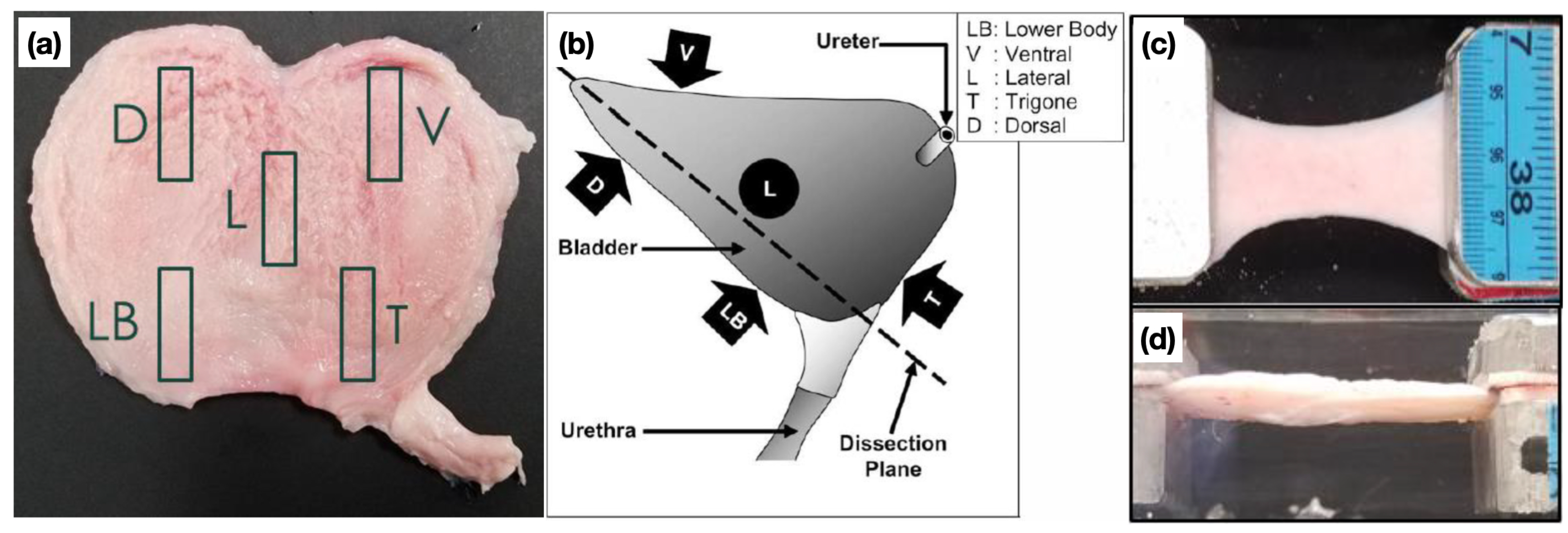
Figure 1. (a) Dissected porcine UB showing the distinct anatomical locations from which samples were punched in the apex-to-base direction. They are denoted as dorsal (D), lateral (L), lower body (LB), trigone (T), and ventral (V). (b) A diagram of the UB from the lateral view. Source: Korossis et al. [18] (c,d) A representative sample under clamped, uniaxial relaxation, respectively, in upper and side views, from which images are extracted for cross-sectional area estimation.
Fractalfract 05 00223 g001
Figure 2. Stress relaxation data for all UB samples. (a,b)—stress vs time data in linear and logarithmic scales. (c,d)—successive step strain vs time data in linear and logarithmic scales. The long-term power-law behavior becomes evident especially in the first relaxation step in (b), where the slope of the black line is given by | β | 0.3 , indicating an anomalous behavior of predominantly elastic nature.
Fractalfract 05 00223 g002
Figure 3. Relaxation moduli for each bladder specimen under distinct applied strains: (a) D, (b) L, (c) LB, (d) T, (e) V. The relaxation behavior seems to be approximately linear for most specimens in the ε i [ 0.25 , 0.5 ] range. All specimens clearly demonstrate a dependency of both time and applied strains for ε i > 0.5 , with largest variations observed in the LB and T samples. Furthermore, the data indicates two distinct relaxation regimes with slower ( t < 3 [s]) and faster ( t > 400 [s]) decays, respectively, with slopes β 1 and β 2 illustrated in (f). The vertical bars represent the average relaxation slopes for each specimen over the 5 applied strain steps, and error bars are computed over one standard deviation from the average value.
Fractalfract 05 00223 g003
Figure 4. Relaxation functions G ( t ) for the building block models under varying fractional models and E 1 = 1 , E 2 = 1 . (a) Scott-Blair, (b) Fractional Kelvin-Voigt, and (c) Fractional Maxwell. We note the progression from a single, scale-free power-law behavior for the SB model to two dominating, asymptotic power-laws under small and large times for the FKV and FM models. Furthermore, the parallel/serial combinations for the FKV/FM models determine whether slower/faster relaxation rates emerge around an intermediate regime, which is characterized by a critical region.
Fractalfract 05 00223 g004
Figure 5. Obtained linear viscoelastic fits for (a) the fractional SB model, and (b) fractional Maxwell model for all bladder samples and the first strain step ( ε 0 = 0.25 ) . The results clearly show the capability of the FM model to better capture the short and long time relaxation regimes of the UB, reinforcing the qualitative agreement observed between the experimental relaxation curves in Figure 3 and the models in Figure 4.
Fractalfract 05 00223 g005
Figure 6. Obtained pointwise errors for the linear SB and FM models for the first strain step: (a) D, (b) L, (c) LB, (d) T, (e) V. Generally, smaller errors are obtained for short and long time behaviors using the FM model, with similar errors for the intermediate time range.
Fractalfract 05 00223 g006
Figure 7. Obtained fits for the fractional QLV model under all strain steps: (a) D, (b) L, (c) LB, (d) T, (e) V. The fit quality was very good for all bladder samples, with more significant deviations occuring on strain steps 4 and 5. The recovered fractional-orders in (f) are within the 0.2 < α < 0.3 range, which is in accordance with the a-priori power-laws obtained from the relaxation moduli data in Figure 3.
Fractalfract 05 00223 g007
Figure 8. Obtained pointwise errors for the FQLV model under all strain steps: (a) D, (b) L, (c) LB, (d) T, (e) V. The vertical gray lines represent the step strain application instants.
Fractalfract 05 00223 g008
Table 1. Obtained material parameters for all employed linear fractional models and UB samples. The range of α 1 values agrees with the power-law exponent range from the experimental relaxation functions in Figure 3.
ModelParametersError %Sample
E 1  [kPa.s α 1 ] α 1 E 2  [kPa.s α 2 ] α 2 LS RMS
SB18.19010.2264.321.72D
FKV15.65740.2252.420190.2294.321.72
FM14.76160.1713976.900.7432.290.91
SB31.30770.2193.471.42L
FKV31.34620.22000.5033.471.41
FM26.93110.18648,826.10.9322.080.82
SB41.63350.2365.331.98LB
FKV33.20050.2327.954290.2525.341.99
FM33.08530.18337,339.90.9353.231.20
SB66.76890.27811.13.82T
FKV66.47140.27800.90711.13.83
FM42.43380.17036,938.70.9994.051.37
SB34.92540.2203.211.24V
FKV34.92540.22000.5793.211.25
FM30.76050.18819,799.50.7972.190.84
Table 2. Obtained material parameters for the FQLV model with all UB samples and employed consecutive strain steps, with range of α 1 values also in agreement with power-law exponents from Figure 3.
SampleParametersError %
A [kPa]BE [s α ] α LSE RMSE
D53.88230.78030.72980.29284.851.11
L79.16460.88230.56770.26734.081.00
LB74.53691.21920.34630.25104.171.00
T63.44351.26420.35900.24195.611.44
V59.32820.94490.67040.27324.741.16
Publisher’s Note: MDPI stays neutral with regard to jurisdictional claims in published maps and institutional affiliations.