1. Introduction
Many real-life networks, such as hyperlinks in the World Wide Web, protein–protein interaction networks and cellular networks [
1,
2,
3], exhibit fractal and scale-free characters, and models for fractal scale-free networks have been a research hotpot [
3,
4,
5,
6,
7,
8,
9]. The self-similar structures of these networks make it possible for us to analytically evaluate the topological and dynamic properties of these networks. Among a plethora of dynamic processes, the first-passage process is of particular important since many other dynamic processes can be analyzed and understood in terms of a first-passage process [
10,
11,
12]. Typical examples include fluorescence quenching, where light emission stops when it reacts with a quencher; the stopping of the searching process for a wandering forager when it first reaches the target; and gene expression where the cell division event occurs when the copy number of the time-keeper protein hits a threshold for the first time [
13,
14]. An important quantity related to the first-passage process is the mean first-passage time (MFPT), referred to as
, which is the expected time for a walker starting from site
i to reach the target
j for the first time. Averaging the MFPT over all the possible source and target sites, one can obtain the global mean first-passage time (GMFPT), referred to as
and defined by
where
N is the total number of nodes of the underling networks.
In the past several decades, the first-passage properties have attracted lots of attention [
15,
16,
17,
18], and the mean first-passage time has been extensively studied. Some of them focus on disclosing the effects of the topology on the MFPT (or GMFPT), and lots of results have been obtained for unbiased random walks on different networks, such as Sierpinski gaskets [
19,
20], pseudofractal scale-free web [
21,
22], scale-free Koch networks [
9,
23],
flowers [
24], and many fractal scale-free trees [
9,
21,
25,
26,
27]. The MFPT and GMFPT are useful indicators for the transport efficiency of the network. These works uncovered the effects of the topology on the transport efficiency. There are also many works devoted to improving the transport efficiency by designing appropriate biased random walk strategies [
28,
29,
30]. By introducing the proper weight to each edge of the network and designing a proper biased random walk strategy, one can shorten the MFPT to obtain higher transport efficiency on the underling networks [
31,
32,
33,
34,
35]. One can also shorten the GMFPT for random walks on some networks [
36].
In this work, we extend the networks studied in Refs. [
25,
36] to a kind of general fractal scale-free trees, which are controlled by two integer parameters:
u and
v . The networks in the case
(or
) are just the networks studied in Refs. [
25,
36]. Here, we study unbiased and biased random walks on the general fractal scale-free trees (FSTs), aiming at shortening the GMFPT and optimizing the transport efficiency of the networks. Firstly, we analyze the GMFPT for classical unbiased random walks on the FSTs. Then, we introduce the proper weight to each edge of the FSTs and design a proper biased random walk strategy, then evaluate the GMFPT analytically for biased random walks on the FSTs. Finally, we compare the results of the GMFPT for unbiased random walks and those for biased random walks and find the effects of the weights on the GFMPT. The way to shorten and minimize the GMFPT is found. Therefore, we obtain a way to optimize the first-passage process for random walks on the general fractal scale-free trees.
This paper is organized as follows. In
Section 2, we describe the typologies of the fractal scale-free trees and the weighted fractal scale-free trees. Next, in
Section 3, we evaluate the GMFPT for classical unbiased random walks on the FSTs. In
Section 4, we analyze the GMFPT for biased random walks on the FSTs. In
Section 5, we compare the GMFPT for unbiased random walks and the GMFPT for biased random walks on the FSTs and present the optimal parameters where the GMFPT achieves its minimum. Finally, conclusions and discussions are provided in
Section 6, and detailed derivations are collected in the Appendixes.
2. Fractal Scale-Free Trees and the Weighted Fractal Scale-Free Trees
The networks considered here are deterministic networks that can be built in an iterative way. Let
denote the network of generation
n . The construction starts from two nodes connected by an edge, which corresponds to
. For
,
can be obtained from
in the following way. For each edge of
, we replace it with a path of length
u firstly, and then
new nodes are added; half of them are connected to one endpoint of the path and half of them are connected to another endpoint of the path. For convenience, we call the
new nodes with degree 1 as external nodes and the
new nodes in the path with length
u as internal nodes. In other words,
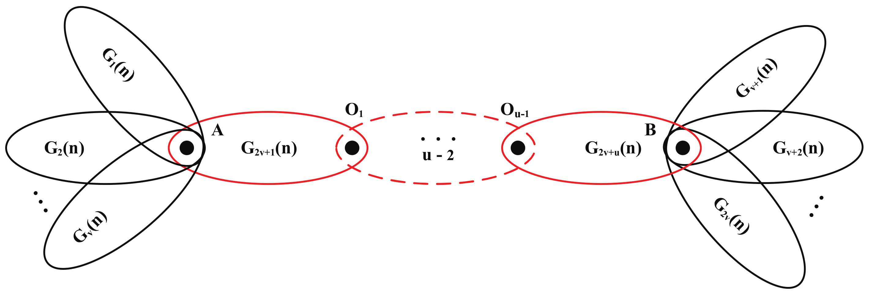
can be obtained from
by replacing each edge of
with the cluster on the right-hand side of
Figure 1. The networks for the particular case
and
are just the networks studied in Refs. [
25,
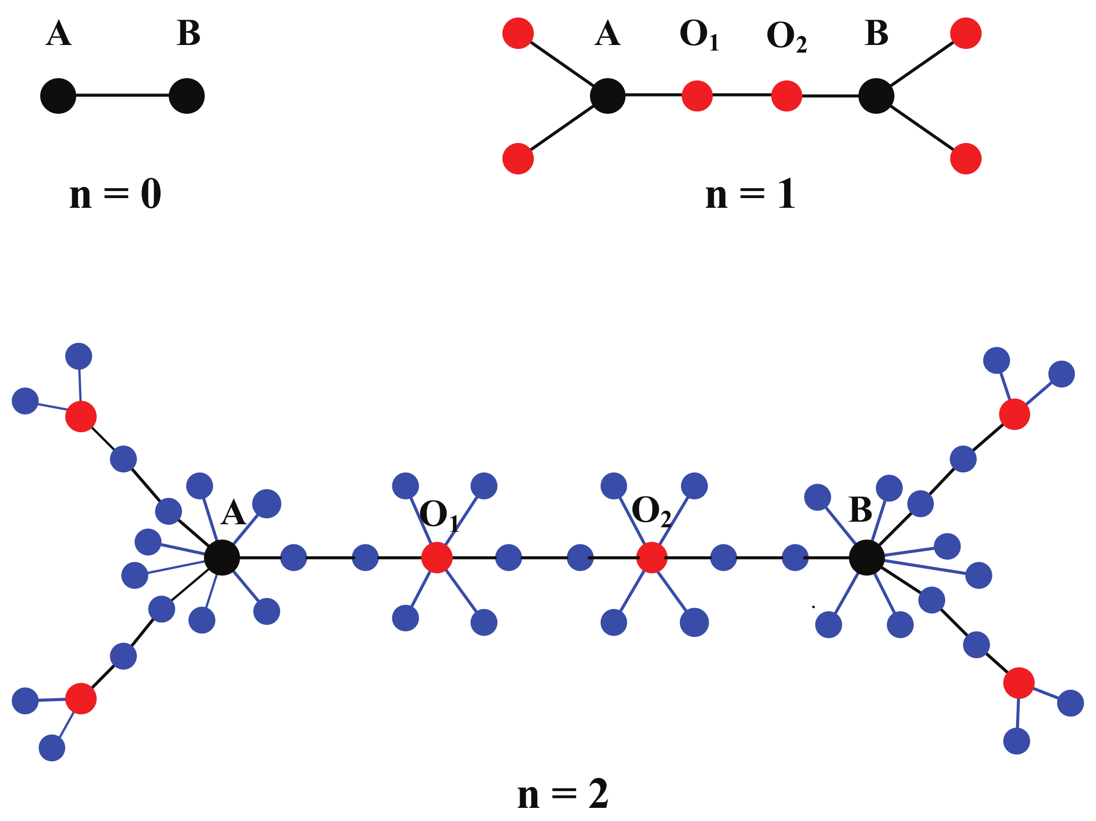
36]. The construction process for the first three generations of the network in the particular case of
are shown in
Figure 2.
According to the construction, we can easily know the total number of edges
of
is
and the total number of nodes
is
One can also find that, in the case
, these kinds of networks are non-fractal, which means that they have infinite fractal dimension; and in the case of
, they are fractals with the fractal dimension
[
7]. Further more, they are scale-free trees with the distribution
, where
[
7]. Therefore, in the case
, we can call them fractal scale-free trees (FSTs).
Note that the first-passage properties for the networks with
and
were studied in Refs. [
25,
36]. In this paper, we just study the networks while
. We study the tree-like networks because of their inherent interests and their correlation with real systems, where the so-called boundary tree is well known [
37,
38].
It is worth mentioning that the networks considered here have an equivalent construction method that highlights their self-similarity. As shown in
Figure 3, the network with generation
, referred to as
, is composed of
sub-units that are copies of
, labeled by
, and connected to one another by their hubs (i.e., nodes with highest degree).
In order to construct the biased random walk strategy, we introduce weight to each edge of the fractal scale-free trees and obtain the weighted fractal scale-free trees in the following recursive way. For
, the weight for the only edge of
is 1. For
, it is known that
is obtained from
by replacing each edge of
with a path of length
u firstly, and then
new nodes are added; half of them are connected to one endpoint of the path and half of them are connected to another endpoint of the path. The weights for edges of
can be also obtained from the weights for edges of
. The weights for the
u new edges in the path with length
u are the same as the weights for the original edge of
, and the weights for the edges between the endpoints of the path and the
new nodes are set to be
w times the weight of the original edge. Therefore,
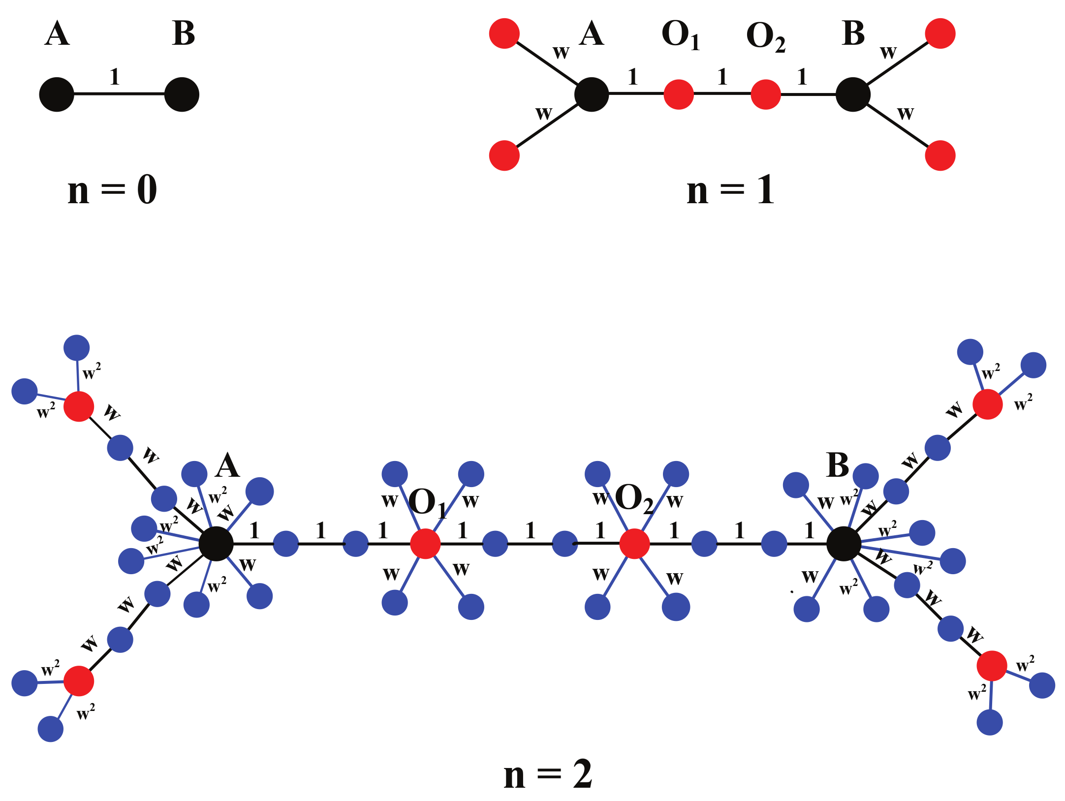
w is an important parameter that controls the weights for the edges of the networks. The weights for edges of the particular fractal scale-free trees in
Figure 2 are shown in
Figure 4.
3. GMFPT for Unbiased Random Walk on the Fractal Scale-Free Trees
In this section, we analyze the GMFPT for classical unbiased random walks on fractal scale-free trees (FSTs). At any step, the walker at the current site
i steps to any of its neighbors
j with the same probability. This is to say, the transition probability from node
i to node
j can be written as
where
is the degree of node
i, and
means there is an edge between nodes
i and
j.
In order to show the evolution of the global mean first-passage time with the increase in the network size, here,
represents
for network
. By exploring the connection between the MFPT and the effective resistance and the relation between the effective resistance and the shortest path length, the global mean first-passage time (GMFPT), defined by Equation (
1), for unbiased random walks on network
can be rewritten as [
25]
where
and
denotes the shortest path length between nodes
i to node
j on network
.
Note that
is just two nodes connected by an edge. It is easy to know
. For
, recalling the self-similar structure of fractal scale-free trees, as shown in
Figure 4, the
is composed by
subunits, which are copies of
, labeled by
and connected to one another by their hubs. We have
where
is the sum of shortest path between any two nodes that belong to the different subunits of
.
Using the Equation (
7) recursively, for
, we obtain
Inserting Equation (
9) into Equation (
8), we obtain
Replacing
from Equation (
10) in Equation (
5), we obtain
Noticing that
and
, we can rewrite Equation (
11) as
Therefore, for large networks, i.e.,
,
4. GMFPT for Biased Random Walk on the Weighted Fractal Scale-Free Trees
In this section, we analytically evaluate the GMFPT for biased random walks on the weighted fractal scale-free trees. At any step, the transition probability from node
i to
j is
where
is the set of neighbors of node
i, and
is the weight of the edge between nodes
i and
j.
If we view the weighted fractal scale-free trees as electrical networks by considering any edge
between two adjacent nodes
i and
j to be a resistor with resistance
. We find, for any
, the GMFPT for biased random walks on the weighted fractal scale-free trees
can be expressed as [
36]
where
is the sum of weights for all edges of the weighted fractal scale-free trees
, and
, with
is the the resistances between nodes
i and
j on
. In order to derive
, we should calculate
and
.
Firstly, we calculate
. It is easy to know
. For any
, as shown in
Figure 4, the
is composed by
subunits, which are copies of
, labeled by
. Furthermore, the edge weights for subunits
are the same as those of
, whereas the weight for each edge of subunits
is
w times the weight for the corresponding edge of
. We obtain
where
, and
is the sum of the effective resistance between any two nodes that belong to the different subunits of
.
Using Equation (
16) recursively, we obtain
For
, we find
where the detailed derivation of Equation (
18) is presented in
Appendix B.
Therefore, inserting Equation (
18) into Equation (
17), we obtain
Then, we calculate the
, which is the sum of weights for all edges of
. For
, we find
. For
, we find
Replacing
and
from Equations (
19) and (
21), respectively, we obtain
Let
in Equation (
22), then we can recover the result, as shown in Equation (
11), which is the GMFPT for the unbiased random walk on
. Let
in Equation (
22), then we can recover the result obtained in Ref. [
36]. They all confirm the correctness of our results.
5. Optimizing the First-Passage Process by Using the GMFPT as the Measure
In this section, we analyze the effect of weight parameter w on , and then find the optimal w where achieves its minimum. Therefore, we obtain a random walk strategy to speed up the first-passage process on the FSTs.
Recalling the exact result of the GMFPT, as shown in Equation (
22), for a biased random walk on the weighted networks, we find for a network that is big enough, i.e,
, Equation (
22) can be rewritten as
Therefore, if
,
and if
,
Noticing that
, we can rewrite
as
Figure 5 and
Figure 6 show the double logarithmic plots of
versus
for different choices of
w in the case
,
,
,
and
, respectively. They all confirm the asymptotic behavior in Equation (
26).
Considering the power exponent of
, as shown in Equation (
26), one can find that
decreases monotonically in
w if
, whereas
increases monotonically in
w if
. Thus,
decreases monotonically as
w increases if
, whereas
increases monotonically in
w if
. Therefore,
reaches its minimum at
.
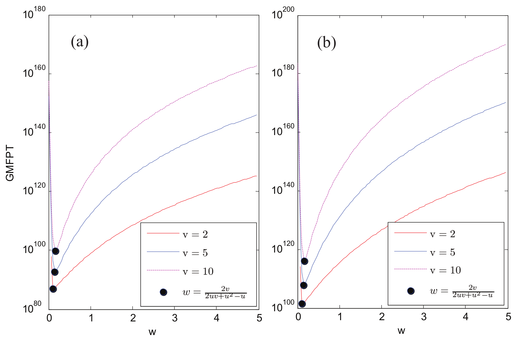
Figure 7 and
Figure 8 shows the plots of
versus
w for different
v in the case that
(
) and
. In all the cases,
reaches its minimum at
.
Letting
in Equation (
26), we obtained the optimal
, which scales as
In order to show the improvement on the GMFPT of our optimal solution obtained here, the ratio between the optimal GMFPT
and the GMFPT for an unbiased random walk, as obtained in
Section 3 and referred to as
, is evaluated, and it scales with the size of the network as
We have red
, and for large networks, i.e.,
,
Therefore, the optimal biased random walk strategy presented here shortens the GMFPT in comparison to the classical unbiased random walk strategy.
6. Conclusions
In this work, we considered a class of recursively grown networks, whose topology is controlled by two integral parameters
u and
v. These kinds of networks provide an interesting model for self-similar and scale-free networks in real life. They can also be used as a candidate structure for the artificial polymer material that has a self-similar structure with a different fractal dimension. In particular, networks in the cases of
and
constitute the formal models studied in Ref. [
25].
Here, we have analytically evaluated the GMFPT for unbiased (and biased) random walks on these networks. The exact results of the GMFPT for unbiased and biased random walks are both obtained. The results show, in both cases, the GMFPTs are power functions in network size .
For an unbiased random walk strategy,
if
. For the biased random walk strategy, it is controlled by a weight parameter
w , and for big networks,
can be looked upon as a convex function of
w, which has an inflection point at
. Therefore, for big networks,
achieves its minimum at
, and we obtain a way to speed up the first-passage process on fractal scale-free trees. The main reason is as follows.
is proportional to the sum of effective resistances for the paths between all pairs of nodes in the network. For two arbitrary nodes, the path can be divided into two types: the first type must pass through at least one internal part, denoted by
, the other type does not pass through any internal parts, denoted by
. Then
is relevant to
, which is independent of
w, and
is subject to parameter
w. As found in
Appendix B,
scales with
n as
, whereas
scales with
n as
. In the asymptotic limit (i.e.,
), only
or
is dominant in
. If
, equivalently,
, we have
, and Equation (
25) holds. On the contrary, if
, we have
, and Equation (
24) holds. Therefore,
is just the inflection point of
with respect to
w.
The results obtained here provide interesting hints for the design of a polymer embedding diffusion process. First, one can construct a class of polymers with different fractal dimensions and different transport efficiencies. The bigger the fractal dimension, the slower the transport on the networks. One can also improve the transport efficiency of the polymer by properly adjusting the weights of each edge.
In future research, we can also set the weight which is related to the node degree, for example, , where and is the degree of node i, j. How we to optimize the first-passage process in this case is an interesting problem.


