Article

Fractal Calculus on Fractal Interpolation Functions

by
Arulprakash Gowrisankar
1,†,
Alireza Khalili Golmankhaneh
2,*,† and
Cristina Serpa
3,†
1
Department of Mathematics, School of Advanced Sciences Vellore Institute of Technology, Vellore 632 014, Tamil Nadu, India
2
Department of Physics, Urmia Branch, Islamic Azad University, P.O. Box 969, Urmia, Iran
3
ISEL—Instituto Superior de Engenharia de Lisboa and CMAFcIO—Centro de Matemática, Aplicações Fundamentais e Investigação Operacional, 1749-016 Lisboa, Portugal
*
Author to whom correspondence should be addressed.
These authors contributed equally to this work.
Fractal Fract. 2021, 5(4), 157; https://doi.org/10.3390/fractalfract5040157
Submission received: 1 September 2021 / Revised: 29 September 2021 / Accepted: 2 October 2021 / Published: 8 October 2021
(This article belongs to the Section Engineering)

Abstract

:
In this paper, fractal calculus, which is called F α -calculus, is reviewed. Fractal calculus is implemented on fractal interpolation functions and Weierstrass functions, which may be non-differentiable and non-integrable in the sense of ordinary calculus. Graphical representations of fractal calculus of fractal interpolation functions and Weierstrass functions are presented.

1. Introduction

It is well known that many phenomena in nature are modeled using fractals [1,2,3,4,5,6,7,8]. The geometrical structures and properties of irregular objects were narrated by Mandelbrot. He termed this as fractal, and it plays a vital role in nonlinear analysis [9]. A fractal is constructed as a non-empty compact invariant set, which is a unique fixed point of a given set of contraction mapping in a complete metric space. This unique fixed point is, in generally, called a deterministic fractal or attractor of the iterated function system (IFS).
The classical interpolation theory investigates the existence and reconstruction of a continuous function that fits the prescribed data. In general, the traditional interpolation methods generate smooth or piecewise differentiable functions despite given data that is irregular. Along these lines, existing non-fractal methods are not appropriate to describe naturally occurring functions. To conquer this circumstance, Barnsley constructed an interpolation function with the notion of an iterated function system, which is an improvement and generalization over the interpolation methods [10].
The concept of a fractal interpolation function (FIF) was developed on this iterated function system, which initiated a new research field in interpolation/approximation theory [11,12,13]. Due to the modern utilization of fractal interpolation functions in approximating non-smooth functions, extensive research has been established in this realm—for instance, new types of FIF are constructed by choosing diverse iterated function systems (see [14,15,16,17,18]).
In addition to bringing the best approximation to the given data, researchers usually demand that interpolation or approximation methods ought to speak to the physical reality beyond what many would possibly consider. Fractal interpolation functions produce complicated mathematical structures/naturally occurring functions with a simple recursive procedure, and thus the fractal approach provides flexibility and versatility in approximation. Though the approximation of a continuous function regarding a polynomial is given by the Weierstrass theorem, approximating a non-smooth function is significant, as objects in the universe, in general, abound in the class of everywhere continuous and nowhere differentiable functions.
Hence, numerous researchers have given more consideration as of late to the problem of how to depict non-smooth functions through the fractal interpolation function from various viewpoints. Moreover, approaches have been established to analyze the non-smooth functions with various aspects.
A general framework between fractional calculus and fractal functions by giving the relation between the fractal dimension of random function and the order of fractional calculus is narrated in [19,20,21,22]. A linear connection between the order of the fractional calculus and the dimensions of the graph of the Weierstrass functions was investigated [23]. Further, the fractional integral of a linear fractal interpolation function and its box dimension were explored in [24].
Similarly, there have been continuous efforts portrayed to analyze the fractal dimensions and order of fractionals [25,26,27,28,29]. Anomalous diffusion was studied by fractional diffusion equations that lead to power low mean square displacement [30,31]. The Lévy-walk model was used to generate anomalously fast diffusion and a finite velocity of a random walker [32,33]. Analysis on fractals was formulated using measure theory, Brownian motion, harmonic analysis, fractional spaces, time scale, and non-standard analysis [34,35,36,37,38,39,40,41,42,43,44].
Although every one of these topics has expanded our comprehension and produced numerous excellent associations, an immediate and straightforward procedure including fractional order operators on fractals was only recently investigated. Despite the fact that the measured theoretical approach is exquisite, Riemann integration-like procedures have their own place. They are more straightforward, constructive, and advantageous according to algorithmic perspective. Occasionally, numerical calculation algorithms on Lebesgue integrals are put together more regularly with respect to Riemann sums.
Hence, A.D. Gangal and coworkers tuned calculus to measure the theoretical approach and systematically explained a series of calculus on fractals involving integrals and derivatives of appropriate orders in between 0 and 1 (refer to [45,46,47]). This has been generalized to different fractal spaces and applied in physics and non-equilibrium statistical mechanics [48,49,50,51]. In this paper, the fractal integral is applied on the fractal interpolation function; hence, the function must be continuous. In order to make a fractal function continuous, it must obey the joint conditions even though these conditions are a particular case of the so-called compatibility conditions in [12,52,53].
The present work is organized as follows: The mathematical background of fractal calculus is elaborated in Section 2. The fractal calculus of Weierstrass functions is presented in Section 2.1. The theoretical background of fractal interpolation functions and their basic construction is established in Section 3. In Section 4, the fractal calculus of a fractal interpolation function is investigated, and examples with graphical representation are presented. Section 5 is devoted to our conclusions.

2. Fractal Calculus

In this section, we briefly recall the requisite general material of fractal calculus. For a detailed exposition, the reader may refer to [45,46,47,48,49,50,51]. The generalization of fractal curves has been formalized. Continuity is not an intrinsic characteristic of fractals. However, in the method of interpolation, as is defined in the literature, the functions are required to be continuous. The key to obtaining continuity is the so-called joint conditions. These conditions are a particular case of the so-called compatibility conditions, which were defined in [12] and developed in [52]. There are two methods to obtain fractals functions from real data: fractal interpolation and the fractal regression [53].
Fractal curves are often defined as images of continuous functions f from R to R n , which are fractals. A fractal curve F R n is said to be parametrizable if there exists a function w : R F , which is continuous, one-to-one, and onto. A subdivision P [ a , b ] (or simply P) of the interval [ a , b ] is a finite set of points { a = x 0 , x 1 , , x n = b } , x i < x i + 1 . Any interval of the form [ x i , x i + 1 ] is called a component of the subdivision P.
Definition 1.
Let F be a fractal curve and P [ a , b ] be a subdivision. The mass function is defined as [46]
γ α ( F , a , b ) = lim δ 0 inf { P [ a , b ] : | P | δ } i = 1 n 1 | w ( t i ) w ( t i + 1 ) | α Γ ( α + 1 ) ,
where | . | is applied to images of w, 1 < α 2 , and the range of w is R n , then this would be the Euclidean metric on R n and
| P | = max 0 i n 1 ( t i + 1 t i )
for a subdivision P.
Definition 2.
The staircase functions for the fractal curve are defined by [46]
S F α ( t ) = γ α ( F , p 0 , t ) , t p 0 , γ α ( F , t , p 0 ) , t < p 0 ,
where p 0 [ a , b ] is an arbitrary and fixed point.
Definition 3.
The γ-dimension of the fractal curve F is defined as [46]
dim γ ( F ) = inf { α : γ α ( F , a , b ) = 0 } = sup { α : γ α ( F , a , b ) = } .
Definition 4.
The F α -derivative of a function f at θ F is defined as [46]
d F α f ( θ ) = F lim θ θ f ( θ ) f ( θ ) J ( θ ) J ( θ ) ,
where J ( θ ) = S F α ( w 1 ( θ ) ) , θ F and if the limit exists.
A segment C ( t 1 , t 2 ) of the fractal curve is defined as [46]
C ( t 1 , t 2 ) = { w ( t ) : t [ t 1 , t 2 ] } .
Definition 5.
The F α -integral of the function f is defined as [46]
C ( a , b ) f ( θ ) d F α θ = C ( a , b ) ̲ f ( θ ) d F α θ = C ( a , b ) ¯ f ( θ ) d F α θ .

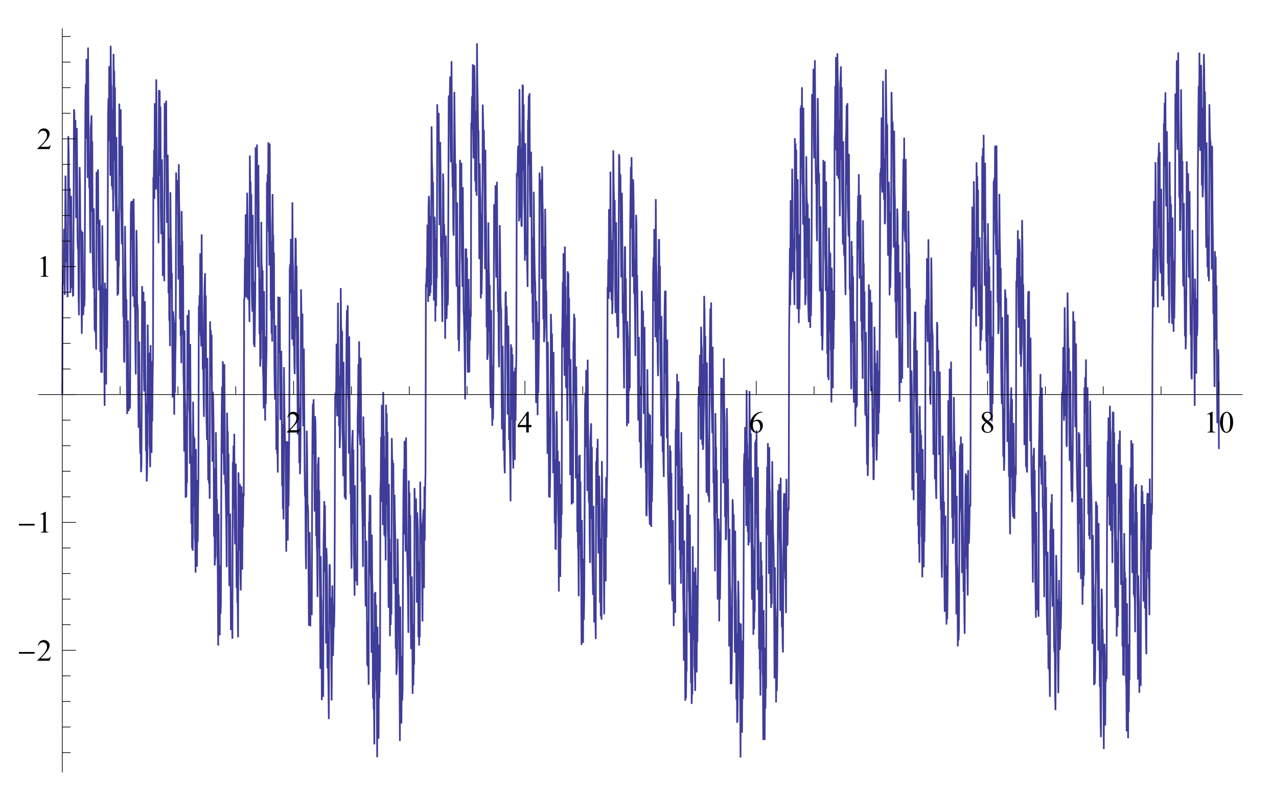
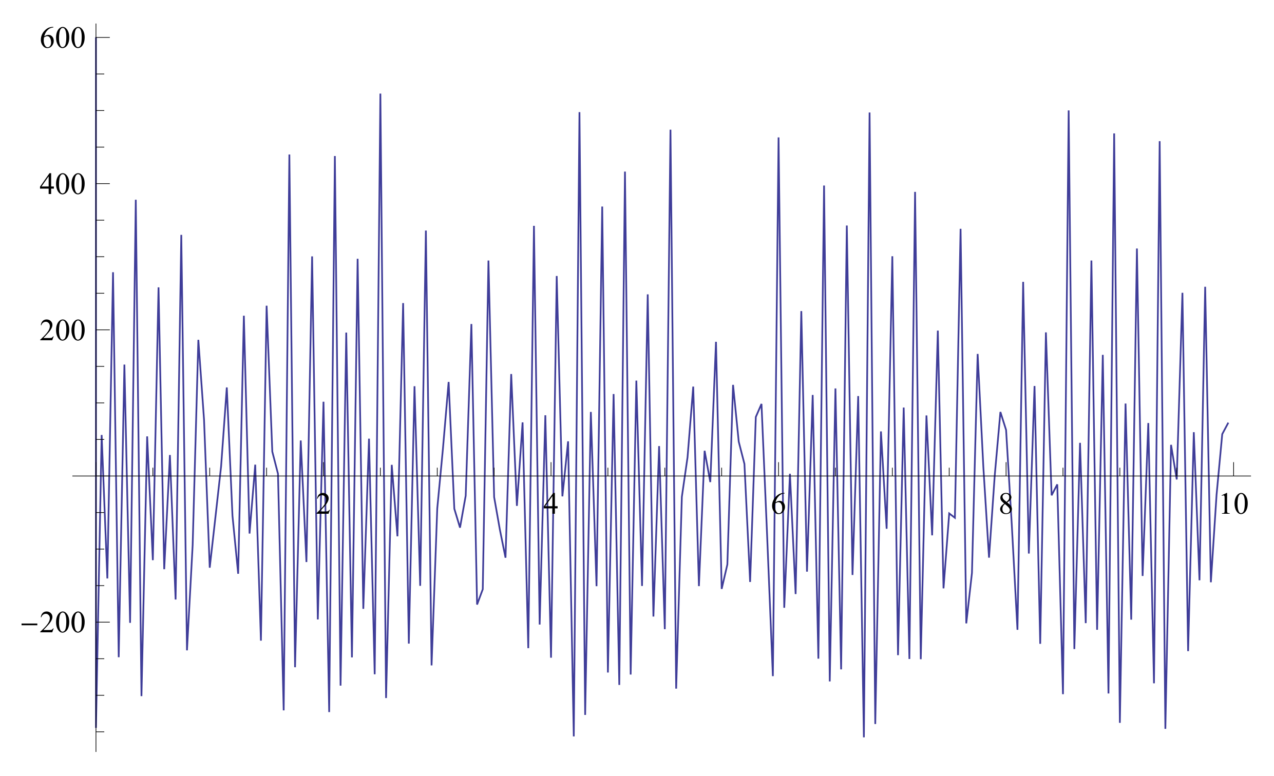
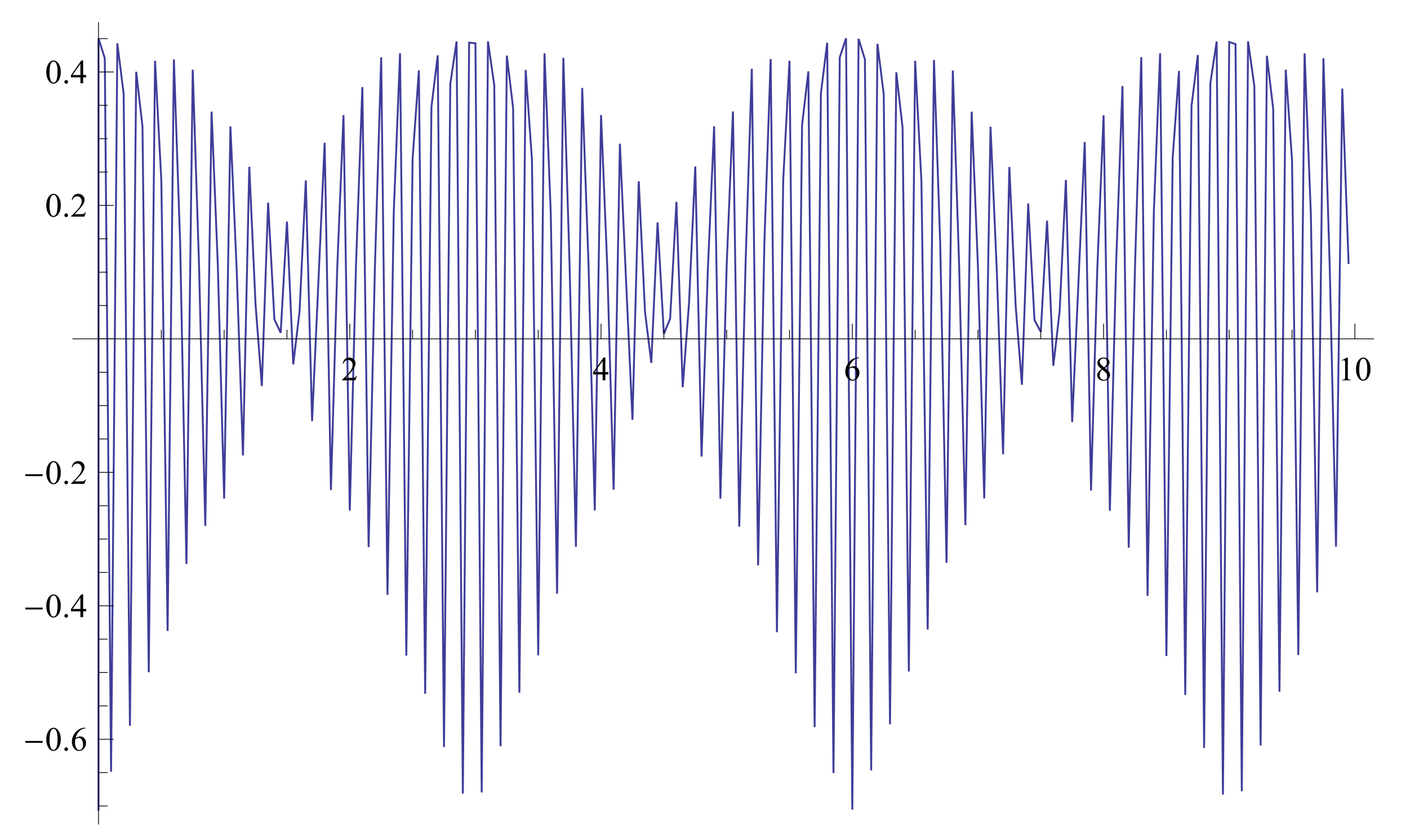
2.1. Fractal Calculus of the Weierstrass Function

For example, w : R R 2 is defined by w ( t ) = ( t , W λ s ( t ) ) where W λ s ( t ) is the Weierstrass function, which is defined by
W λ s ( t ) = k = 1 λ ( s 2 ) k sin ( λ k t )
where λ > 1 and 1 < s < 2 .
The fractal derivative of Weierstrass functions using conjugacy of fractal calculus with ordinary calculus is given by [47]:
D F α W λ s ( t ) = 1.7411 cos ( 2 S F α ( t ) ) + 3.03143 cos ( 4 S F α ( t ) ) + 5.27803 cos ( 8 S F α ( t ) ) + 9.18959 cos ( 16 S F α ( t ) ) + 16 . cos ( 32 S F α ( t ) ) + 27.8576 cos ( 64 S F α ( t ) ) + 48.5029 cos ( 28 S F α ( t ) ) + 84.4485 cos ( 256 S F α ( t ) ) + 147.033 cos ( 512 S F α ( t ) ) + 256 cos ( 1024 S F α ( t ) ) +
The fractal integral of a Weierstrass function is given by
W λ s ( t ) d F α ( t ) = 0.870551 cos ( S F α ( t ) ) 2 0.189465 cos ( 4 S F α ( t ) ) 0.0824692 cos ( 8 S F α ( t ) ) 0.0358968 cos ( 16 S F α ( t ) ) 0.015625 cos ( 32 S F α ( t ) ) 0.00680118 cos ( 64 S F α ( t ) ) 0.00296038 cos ( 128 S F α ( t ) ) 0.00128858 cos ( 256 S F α ( t ) ) 0.000560888 cos ( 512 S F α ( t ) ) 0.000244141 cos ( 1024 S F α ( t ) )
Figure 1 sketches the graph of the Weierstrass function, and Figure 2 and Figure 3 elucidate the fractal derivative and fractal integral of the Weierstrass function.

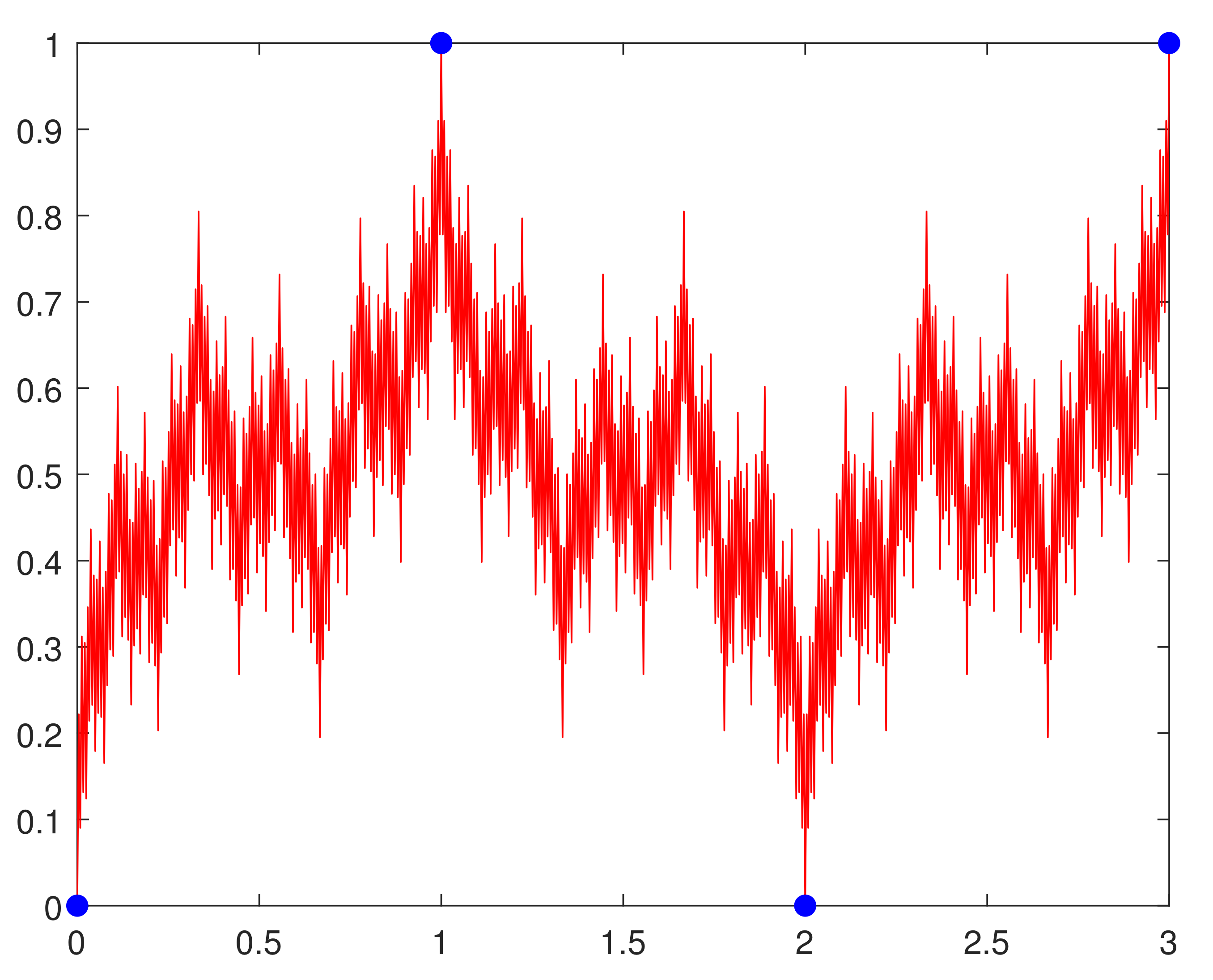
3. Fractal Interpolation Functions

This section provides the theoretical background of the fractal interpolation functions and establishes their basic construction, which is required for the subsequent sections. For more details, readers are directed to [10,11,12,13,14,52].

3.1. The Original Formulation

For N N , let N N denote the subset { 1 , 2 , , N } of N . Let a set of data points { ( x i , y i ) R 2 : i N N } satisfying x 1 < x 2 < < x N , N > 2 , be given. Set I = [ x 1 , x N ] , I i = [ x i , x i + 1 ] for i N N 1 . Let L i : I I i , i N N 1 be contraction homeomorphisms satisfying the endpoint condition
L i ( x 1 ) = x i , L i ( x N ) = x i + 1 .
Let 0 < r i < 1 , i N N 1 , and X : = I × R . Let N 1 continuous mappings R i : X R such that
R i ( x 1 , y 1 ) = y i , R i ( x N , y N ) = y i + 1 , | R i ( x , y ) R i ( x , y * ) | r i | y y * | ,
where ( x , y ) , ( x , y * ) X . Define functions f i : X I i × R , f i ( x , y ) = L i ( x ) , R i ( x , y )   i N N 1 . It is known that there exists a metric on R 2 , equivalent to the Euclidean metric, with respect to which f i , i N N 1 , are contractions. The collection { X ; f i : i N N 1 } is called an Iterated Function System (IFS). Associated with the IFS { X ; f i : i N N 1 } , there is a set-valued Hutchinson map F : H ( X ) H ( X ) defined by
F ( B ) = N 1 i = 1 f i ( B )
for B H ( X ) , where H ( X ) is the set of all nonempty compact subsets of X endowed with the Hausdorff metric H d . The Hausdorff metric H d completes H ( X ) . Further, F is a contraction map on the complete metric space ( H ( X ) , H d ) . By the Banach Fixed Point Theorem, there exists a unique set G H ( X ) such that F ( G ) = G . This set G is called the attractor corresponding to the IFS { X ; f i : i N N 1 } . The attractor G is the graph of a continuous function g : I R , which obeys g ( x i ) = y i for i N N . The function g whose graph is the attractor of an IFS is called a Fractal Interpolation Function (FIF) corresponding to the IFS { X ; w i : i N N 1 } .
The fractal interpolation function g, which is obtained as the fixed point of the Read–Bajraktarević (RB) operator T on a complete metric space ( G , δ ) , is defined as
( T h ) ( x ) = R i L i 1 ( x ) , h L i 1 ( x ) x I i , i N N 1 ,
where G : = { h : I R | h is continuous on I , h ( x 1 ) = y 1 , h ( x N ) = y N } equipped with the metric δ ( h , h * ) = max { | h ( x ) h * ( x ) | : x I } for h , h * G . It can be seen that T is a contraction mapping on ( G , δ ) with a contraction factor r = max { r i : i N N 1 } < 1 . The fixed point of T is the FIF g corresponding to the IFS. Therefore, g satisfies the functional equation:
g ( x ) = R i L i 1 ( x ) , g L i 1 ( x ) , x I i , i N N 1 .

3.2. System of Iterative Functional Equations

This type of functions may also be obtained as solutions of a system of iterative functional equations (see e.g., [11,12,13,52]). Let X and Y be non-empty sets and p 2 be an integer. Consider a system of functional equations
φ f j x = F j x , φ x , x X j , j = 0 , 1 , p 1 ,
where X and Y are non-empty sets, X j X , f j : X j X , F j : X j × Y Y are given functions, and φ : j = 0 p 1 X j = X Y is the unknown function. It is proven in [11] that the solutions of (9) have a fractal structure.
We consider the affine case
φ x + j p = a j φ x + b j x + c j , x 0 , 1 , 0 j p 1 ,
where a j , b j , c j R are the parameters of the model with a j < 1 , 0 j p 1 .
Parameters a j are the scaling factors or fractal coefficients.
The construction of function solutions of (10) is based on the p-expansion of numbers x 0 , 1 (see [12,13,52]. If the corresponding compatibility conditions (see [12,13,52]) are verified, the function φ solution of (10) is given by
φ n = 1 ξ n p n = n = 1 n 1 k = 1 a ξ k b ξ n m = 1 ξ m + n p m + c ξ n ,
where 0 ξ n p 1 are integers.

4. Fractal Calculus on Fractal Interpolation Function

4.1. With Cantor like Sets Domains

The first example of a fractal F in the theory of fractal calculus is the (ternary) Cantor set. The Cantor set consists of all x 0 , 1 that do not have the digit 1 in their p-expansion. The images of fractal curves φ solutions of (10) are naturally adapted to a domain given by this Cantor set. In fact, the images are obtained from (11) when ξ n 1 , n N . Another Cantor type set may be defined as domains for systems (10), where all elements would be given with one or more missing digits (fixed digits) from their p-expansion.
Definition 6.
Let p 2 be an integer and V 0 , 1 , , p 1 , such that # V = v < p 1 . A Cantor like F is a fractal set defined by
F = n = 1 ξ n p n : ξ n 0 , 1 , , p 1 \ V .
In this setting, the fractal calculus fits very well and the natural subdivisions on Cantor-like set F are as follows:
Definition 7.
A subdivision P 0 , 1 is a finite set of points x i = i / n , 0 i n .
Now, x i + 1 x i = p k , where k N . The definitions of fractal calculus become simpler in the case of a Cantor-like set F.
Definition 8.
For a Cantor-like set F and a subdivision P 0 , 1 , with # P 0 , 1 = n = p k + 1 , P 0 , 1 = p k
σ α F , P = n 1 i = 0 n α 1 Γ α + 1 θ F , i n , i + 1 n ,
where for a closed interval I,
θ F , I = 1 i f   F I = 0 o t h e r w i s e .
Definition 9.
Given δ > 0 , the coarse grained mass γ δ α F , 0 , 1 of F 0 , 1 is given by
γ δ α F , 0 , 1 = inf P 0 , 1 : P 0 , 1 = p k δ σ α F , P = inf P 0 , 1 : P 0 , 1 = p k δ n 1 i = 0 n α 1 Γ α + 1 θ F , i n , i + 1 n .
The ternary Cantor set C has γ -dimension as follows,
dim γ C = ln 2 ln 3 .
Similarly, the γ -dimension of a Cantor-like set F is given by
dim γ F = ln p v ln p .
In these cases, the γ -dimension is equal to both the box and Hausdorff dimensions (see [46]).

4.2. The F α -Integral

We compute the F α -integral of φ solution of (10) with a fractal domain. Before we compute the integral of a FIF, we present an affine change of variables in the F α -integral.
Theorem 1.
Let φ be the solution of (10) with a domain that is a Cantor-like set F as defined in (12). Then,
0 1 φ x + j p d F α x = p α j p j + 1 p φ x d F α x ,
where α = dim γ F and let p 2 be an integer.
Proof. 
The goal is to transform the integral on φ x + j p , by an integral on φ x . An F α -integral may be computed either as
0 1 φ x d F α x = inf P 0 , 1 U α φ , F , P ,
or
0 1 φ x d F α x = sup P 0 , 1 L α φ , F , P ,
where
U α φ , F , P = n 1 i = 0 sup x F i n , i + 1 n φ x S F α i + 1 n S F α i n ,
and
L α φ , F , P = n 1 i = 0 inf x F i n , i + 1 n φ x S F α i + 1 n S F α i n .
We work with the U α φ , F , P . We have
0 1 φ x + j p d F α x = inf P 0 , 1 n 1 i = 0 sup x F i n , i + 1 n φ x + j p S F α i + 1 n S F α i n = inf P 0 , 1 n 1 i = 0 sup x F j p + i p n , j p + i + 1 p n φ x γ α F , 0 , i + 1 n γ α F , 0 , i n .
By the properties of γ α ,
S F α i + 1 n S F α i n = γ α F , 0 , i + 1 n γ α F , 0 , i n = p α γ α 1 p F , 0 , i + 1 p n p α γ α 1 p F , 0 , i p n = p α γ α 1 p F + j p , j p , j p + i + 1 p n γ α 1 p F + j p , j p , j p + i p n = p α γ α F , j p , j p + i + 1 p n γ α F , j p , j p + i p n = p α S F α j p + i + 1 p n S F α j p + i p n .
Then,
0 1 φ x + j p d F α x = p α inf P j p , j + 1 p n 1 i = 0 sup x F j p + i p n , j p + i + 1 p n φ x S F α j p + i + 1 p n S F α j p + i p n = p α j p j + 1 p φ x d F α x .
Theorem 2.
Let φ be the solution of (10) with a domain that is a Cantor-like set F as defined in (12). Then, integral between 0 and 1 of ( φ ( x + j ) / p ) is equal to p α integral ( φ ( x )
0 1 φ ( x ) d F α x = j = 0 , j V p 1 b j 0 1 x d F α x + S F α ( 1 ) j = 0 , j V p 1 c j p α j = 0 , j V p 1 a j
where α = dim γ F and a j , b j , c j are in R and | a j | < 1 .
Proof. 
By definition of φ , for each j 0 , 1 , , p 1 \ V ,
a j 0 1 φ x d F α x = 0 1 φ x + j p d F α x b j 0 1 x d F α x c j 0 1 1 d F α x .
Using the change of variables (13), summing(15) for all j 0 , 1 , , p 1 \ V , and solving the resulting equation in order to 0 1 φ x d F α x , we obtain the desired conclusion. □
Remark 1.
Calculation of 0 1 x d F α x in (14) is done in [47] for the ternary Cantor set. For a general Cantor-like set F, the calculation is similar.
Since the F α -integral is a generalization of the Riemann integral, the integral of φ for the domain 0 , 1 is the following.
Corollary 1.
Let φ be the solution of (10) with domain 0 , 1 . Then,
0 1 φ x d x = j = 0 p 1 b j 2 + c j p j = 0 p 1 a j .

4.3. The F α -Integral as a FIF

This section presents the fractal calculus of the fractal interpolation function defined by the mappings:
L i ( x ) = a i x + b i , R i ( x , y ) = r i y + q i ( x ) , i N N 1 .
Here, 1 < r i < 1 and q i : I R are suitable continuous functions satisfying (5). The parameter r i is called a vertical scaling factor of the transformation f i , and α = ( r 1 , r 2 , , r N 1 ) is the scale vector corresponding to the IFS. Further, F is a fractal curve in Definition 1.
Theorem 3.
If g is the fractal interpolation function associated with ( L i ( x ) , R i ( x , y ) ) : i N N 1 where R i is given in Equation (17) and, for a given y ˜ 1 , we define g ˜ ( x ) = y ˜ 1 + x 1 x S F α ( g ( t ) ) d F α t . Then, g ˜ is the fractal interpolation function associated with { ( L i ( x ) , R ˜ i ( x , y ) ) : i N N 1 } , where, for i N N 1 ,
R ˜ i = a i r i y + q ˜ i ( x ) , a i = x i + 1 x i x N x 1 , q ˜ i ( x ) = y ˜ i a i r i y ˜ 1 + a i x 1 x S F α ( q i ( t ) ) d F α t , y ˜ i + 1 = y ˜ 1 + k = 1 i a k r k ( y ˜ N y ˜ 1 ) + x 1 x N S F α ( q i ( t ) ) d F α t , y ˜ N = y ˜ 1 + k = 1 N 1 a k x 1 x N S F α ( q k ( t ) ) d F α t 1 k = 1 N 1 a k r k .
Proof. 
Define the fractal integral of g at the initial point as
g ˜ ( x ) = y ˜ 1 + x 1 x S F α ( g ( t ) ) d F α t ,
and then
g ˜ ( L i ( x ) ) = y ˜ 1 + x 1 x i S F α ( g ( t ) ) d F α t + x i L i ( x ) S F α ( g ( t ) ) d F α t = y ˜ i + x i L i ( x ) S F α ( g ( t ) ) d F α t .
We apply a change of variable on t by L i ( t ) in the second term. S F α is linear, and, from Equation (17), one can find that
g ˜ ( L i ( x ) ) = y ˜ i + a i x 1 x S F α ( r i g ( t ) + q i ( t ) ) d F α t = y ˜ i + a i r i x 1 x S F α ( g ( t ) ) d F α t + a i x 1 x S F α ( q i ( t ) ) d F α t = y ˜ i + a i r i g ˜ ( x ) y ˜ 1 + a i x 1 x S F α ( q i ( x ) ) d F α x = a i r i g ˜ ( x ) + q ˜ i ( x ) ,
where q ˜ i ( x ) = y ˜ i a i r i y ˜ 1 + a i x 1 x S F α ( q i ( t ) ) d F α t . Hence, g ˜ is also a fractal interpolation function generated by the IFS { L i ( x ) , R ˜ i ( x , y ) ) : i N N 1 } . Note that q ˜ i ( x ) need not be linear. If q ˜ i ( x ) is linear, then the corresponding FIF is called linear FIF. Take x = x N , L i ( x N ) = x i + 1
y ˜ i + 1 = y ˜ i + a i r i ( y ˜ N y ˜ 1 ) + a i x 1 x N S F α ( q i ( x ) ) d F α x y ˜ i + 1 y ˜ i = a i r i ( y ˜ N y ˜ 1 ) + x 1 x N S F α ( q i ( x ) ) d F α x .
We know that y ˜ i + 1 = y ˜ 1 + k = 1 i ( y ˜ k + 1 y ˜ k )
y ˜ i + 1 = y ˜ 1 + k = 1 i a k r k ( y ˜ N y ˜ 1 ) + x 1 x N S F α ( q k ( x ) ) d F α x .
Take i = N 1 ,
y ˜ N = y ˜ 1 + k = 1 N 1 a k r k ( y ˜ N y ˜ 1 ) + x 1 x N S F α ( q k ( x ) ) d F α x y ˜ N y ˜ 1 = k = 1 N 1 a k α k ( y ˜ N y ˜ 1 ) + k = 1 N 1 a k x 1 x N S F α ( q k ( x ) ) d F α x y ˜ N = y ˜ 1 + k = 1 N 1 a k x 1 x N S F α ( q k ( t ) ) d F α t 1 k = 1 N 1 a k r k .
Thus, g ˜ interpolates the new set of data { ( x i , y ˜ i ) : i N N } , where, for each i N N 1 ,
a i = x i + 1 x i x N x 1 y ˜ i + 1 = y ˜ 1 + k = 1 i a k r k ( y ˜ N y ˜ 1 ) + x 1 x N S F α ( q i ( t ) ) d F α t , y ˜ N = y ˜ 1 + k = 1 N 1 a k x 1 x N S F α ( q k ( t ) ) d F α t 1 k = 1 N 1 a k r k .
In Theorem 3, the fractal integral of the fractal interpolation function is studied by predefining the initial condition y ˜ 1 . Whereas, in the following theorem, by predefining the initial condition y ˜ N , the fractal integral of FIF is investigated, and the corresponding new set of interpolation data are explicitly presented. □
Theorem 4.
If g is the fractal interpolation function associated with ( L i ( x ) , R i ( x , y ) ) : i N N 1 where R i is given in Equation (5) and, for a given y ˜ N , we define g ˜ ( x ) = y ˜ N x x N S F α ( g ( t ) ) d F α t . Then, g ˜ is the fractal interpolation function associated with { ( L i ( x ) , R ˜ i ( x , y ) ) : i N N 1 } , where, for i N N 1 ,
R ˜ i = a i r i y + q ˜ i ( x ) , a i = x i + 1 x i x N x 1 q ˜ i ( x ) = y ˜ i + 1 a i r i y ˜ N x x N S F α ( q i ( t ) ) d F α t , y ˜ i = y ˜ N k = i N 1 a k r k ( y ˜ N y ˜ 1 ) + x 1 x S F α ( q i ( t ) ) d F α t , y ˜ 1 = y ˜ N k = 1 N 1 a k x 1 x N S F α ( q k ( t ) ) 1 k = 1 N 1 a k r k .
Proof. 
Define the fractal integral of g at the endpoint as
g ˜ ( x ) = y ˜ N x x N S F α ( g ( t ) ) d F α t ,
and then
g ˜ ( L i ( x ) ) = y ˜ N L i ( x ) x i + 1 S F α ( g ( t ) ) d F α t x i + 1 x N S F α ( g ( t ) ) d F α t = y ˜ i + 1 L i ( x ) x i + 1 S F α ( g ( t ) ) d F α t .
Applying a change of variable on t by L i ( t ) in the second term. S F α is linear, and, from Equation (17), one can find,
g ˜ ( L i ( x ) ) = y ˜ i + 1 a i x x N S F α ( r i g ( t ) + q i ( t ) ) d F α t = y ˜ i + 1 a i r i x x N S F α ( g ( t ) ) d F α t + a i x x N S F α ( q i ( t ) ) d F α t = y ˜ i + 1 a i r i y ˜ N g ˜ ( x ) a i x x N S F α ( q i ( x ) ) d F α x = a i r i g ˜ ( x ) + q ˜ i ( x ) ,
where q ˜ i ( x ) = y ˜ i + 1 a i r i y ˜ N a i x x N S F α ( q i ( t ) ) d F α t . Hence, g ˜ is also a fractal interpolation function generated by the IFS { L i ( x ) , R ˜ i ( x , y ) ) : i N N 1 } . Note that, q ˜ i ( x ) need not be linear. If q ˜ i ( x ) is linear, then the corresponding FIF is called linear FIF. Further, g ˜ interpolates the new set of data { ( x i , y ˜ i ) : i N N } , where, for each i N N 1 ,
a i = x i + 1 x i x N x 1 y ˜ i = y ˜ N k = i N 1 a k r k ( y ˜ N y ˜ 1 ) + x 1 x N S F α ( q i ( t ) ) d F α t , y ˜ 1 = y ˜ N k = 1 N 1 a k x 1 x N S F α ( q k ( t ) ) 1 k = 1 N 1 a k r k .
Let ( 0 , 0 ) , ( 1 / 3 , 1 / 2 ) , ( 2 / 3 , 1 / 2 ) , ( 1 , 0 ) be the given dataset. Then, the fractal interpolation function g passing through the given dataset with vertical scaling factors r 1 = 0.7071 , r 2 = 0.7071 and r 3 = 0.7071 is determined by the iterated function system:
L 1 ( x ) = 1 3 x , R 1 ( x , y ) = 0.7071 y + 0.0976 x , L 2 ( x ) = 1 3 x + 1 , R 2 ( x , y ) = 0.7071 y 0.0976 x + 1 , L 3 ( x ) = 1 3 x + 2 , R 3 ( x , y ) = 0.7071 y + 0.0976 x .
Here, q i ( x ) is selected as a linear function, i.e., q i ( x ) = a i x + b i for i = 1 , 2 , 3 . The fractal interpolation function g of the given dataset is graphically demonstrated in Figure 4. Additionally, the fractal interpolation function g ˜ , which is determined through the iterated function system with the same L i ( x ) and R ˜ i ( x , y ) , is given by
R ˜ 1 ( x , y ) = 0.2357 y + 0.0163 ( S F α ( x ) ) 2 , R ˜ 2 ( x , y ) = 0.2357 y 0.0163 ( S F α ( x ) ) 2 + S F α ( x ) 3 + 0.1378 , R ˜ 3 ( x , y ) = 0.2357 y + 0.0163 ( S F α ( x ) ) 2 + 0.3762 .
Here, the coefficients of IFS are obtained from Theorem 3, and the fractal integral of the fractal interpolation function g is estimated by predefining the initial condition y ˜ 1 = 0 . The fractal integral of order α = 0.5 of fractal interpolation function g is graphically elucidated in Figure 5. The vertical scaling factors of g are r 1 = 0.2357 , r 2 = 0.2357 , r 3 = 0.2357 and fractal integral of g shows smoothness and a self-similar pattern. The dots in Figure 4 represent the given set of data points, and the solid red line provides the corresponding fractal interpolation function. In Figure 5, the blue dots give the new set of data points, and the solid red line presents the fractal integral of FIF.

5. Conclusions

In this paper, fractal calculus was studied and utilized to obtain the fractal integral and derivatives of the Weierstrass functions and the fractal interpolation functions, which are not differentiable in the sense of ordinary derivatives. Using fractal calculus on Weierstrass functions, one can derive the mean square displacement of random walks by considering the Fokker–Planck equation on Weierstrass functions.
Fractal local derivatives and integral will be of interest to explore fractal functions in a future work.

Author Contributions

Investigation and writing A.G., A.K.G. and C.S., funding acquisition C.S. All authors have read and agreed to the published version of the manuscript.

Funding

Cristina Serpa acknowledges partial support from National Funding from FCT-Fundação para a Ciência e a Tecnologia, under the project: UIDB/04561/2020.

Conflicts of Interest

The authors declare no conflict of interest.

References

  1. Blackledge, J.M.; Evans, A.K.; Turner, M.J. Fractal Geometry: Mathematical Methods, Algorithms, Applications; Elsevier: Amsterdam, The Netherlands, 2002. [Google Scholar]
  2. Pesin, Y.B. Dimension Theory in Dynamical Systems: Contemporary Views and Applications; University of Chicago Press: Chicago, IL, USA, 2008. [Google Scholar]
  3. Edgar, G. Measure, Topology, and Fractal Geometry; Springer Science & Business Media: Berlin/Heidelberg, Germany, 2007. [Google Scholar]
  4. Pietronero, L.; Tosatti, E. Fractals in Physics; Elsevier: Amsterdam, The Netherlands, 2012. [Google Scholar]
  5. Massopust, P.R. Fractal Functions, Fractal Surfaces, and Wavelets; Academic Press: Cambridge, MA, USA, 2016. [Google Scholar]
  6. Losa, G.A.; Merlini, D.; Nonnenmacher, T.F.; Weibel, E.R. Fractals in Biology and Medicine; Birkhäuser: Basel, Switzerland, 2005. [Google Scholar]
  7. Schroeder, M. Fractals, Chaos, Power Laws: Minutes from an Infinite Paradise; Courier Corporation: North Chelmsford, MA, USA, 2009. [Google Scholar]
  8. Sandev, T.; Iomin, A.; Kantz, H. Anomalous diffusion on a fractal mesh. Phys. Rev. E 2017, 95, 052107. [Google Scholar] [CrossRef] [PubMed] [Green Version]
  9. Mandelbrot, B.B. The Fractal Geometry of Nature; WH Freeman: New York, NY, USA, 1983; Volume 173. [Google Scholar]
  10. Barnsley, M.F. Fractal functions and interpolation. Constr. Approx. 1989, 2, 303–329. [Google Scholar] [CrossRef]
  11. Serpa, C.; Buescu, J. Fractal and Hausdorff dimensions for systems of iterative functional equations. J. Math. Anal. Appl. 2019, 480, 123429. [Google Scholar]
  12. Serpa, C.; Buescu, J. Constructive solutions for systems of iterative functional equations. Constr. Approx. 2017, 45, 273–299. [Google Scholar] [CrossRef]
  13. Serpa, C.; Buescu, J. Explicitly defined fractal interpolation functions with variable parameters. Chaos Solitons Fractals 2015, 75, 76–83. [Google Scholar] [CrossRef]
  14. Banerjee, S.; Easwaramoorthy, D.; Gowrisankar, A. Fractal Functions, Dimensions and Signal Analysis; Springer: Cham, Switerland, 2021. [Google Scholar]
  15. Navascués, M.A. Fractal polynomial interpolation. Z. Anal. Anwend. 2005, 25, 401–418. [Google Scholar] [CrossRef]
  16. Navascués, M.A. Non-Smooth polynomial. Int. J. Math. Anal. 2007, 1, 159–174. [Google Scholar]
  17. Katiyar, S.K.; Chand, A.K.B.; Saravana, K.G. A new class of rational cubic spline fractal interpolation function and its constrained aspects. Appl. Math. Comput. 2019, 346, 319–335. [Google Scholar] [CrossRef]
  18. Banerjee, S.; Hassan, M.K.; Mukherjee, S.; Gowrisankar, A. Fractal Patterns in Nonlinear Dynamics and Applications; CRC Press: Boca Raton, FL, USA, 2019. [Google Scholar]
  19. Tatom, F.B. The relationship between fractional calculus and fracta. Fractals 1995, 3, 217–229. [Google Scholar] [CrossRef]
  20. Satin, S.; Gangal, A.D. Random walk and broad distributions on fractal curves. Chaos Solitons Fractals 2019, 127, 17–23. [Google Scholar] [CrossRef] [Green Version]
  21. Satin, S.; Gangal, A.D. Langevin equation on fractal curves. Fractals 2016, 24, 1650028. [Google Scholar] [CrossRef] [Green Version]
  22. Kolwankar, K.M.; Gangal, A.D. Fractional differentiability of nowhere differentiable functions and dimensions. Chaos 1996, 6, 505–513. [Google Scholar] [CrossRef] [Green Version]
  23. Yao, K.; Su, W.Y.; Zhou, S.P. On the connection between the order of fractional calculus and the dimensions of a fractal function. Chaos Solitons Fractals 2005, 23, 621–629. [Google Scholar] [CrossRef]
  24. Ruan, H.J.; Su, W.Y.; Yao, K. Box dimension and fractional integral of linear fractal interpolation functions. J. Approx. Theory 2009, 161, 187–197. [Google Scholar] [CrossRef] [Green Version]
  25. Gowrisankar, A.; Uthayakumar, R. Fractional calculus on fractal interpolation function for a sequence of data with countable iterated function system. Mediterr. J. Math. 2016, 13, 3887–3906. [Google Scholar] [CrossRef]
  26. Liang, Y.S.; Zhang, Q. A type of fractal interpolation functions and their fractional calculus. Fractals 2016, 24, 1650026. [Google Scholar] [CrossRef]
  27. Xiao, E.W.; Jun, H.D. Box dimension of Hadamard fractional integral of continuous functions of bounded and unbounded variation. Fractals 2017, 25, 1750035. [Google Scholar]
  28. Gowrisankar, A.; Prasad, M.G.P. Riemann-Liouville Calculus on Quadratic Fractal Interpolation Function with Variable Scaling Factors. J. Anal. 2019, 27, 347–363. [Google Scholar] [CrossRef]
  29. Liang, Y.S. Progress on estimation of fractal dimensions of fractional calculus of continuous functions. Fractals 2019, 27, 1950084. [Google Scholar] [CrossRef]
  30. Sokolov, I.M. Models of anomalous diffusion in crowded environments. Soft Matter 2012, 8, 9043–9052. [Google Scholar] [CrossRef]
  31. Höfling, F.; Franosch, T. Anomalous transport in the crowded world of biological cells. Rep. Prog. Phys. 2013, 76, 046602. [Google Scholar] [CrossRef] [Green Version]
  32. Zaburdaev, V.; Denisov, S.; Klafter, J. Lévy walks. Rev. Mod. Phys. 2015, 87, 483. [Google Scholar] [CrossRef] [Green Version]
  33. Metzler, R.; Jeon, J.H.; Cherstvy, A.G.; Barkai, E. Anomalous diffusion models and their properties: Non-stationarity, non-ergodicity, and ageing at the centenary of single particle tracking. Phys. Chem. Chem. Phys. 2014, 16, 24128–24164. [Google Scholar] [CrossRef] [Green Version]
  34. Lapidus, M.L.; Frankenhuijsen, M.V. Fractal Geometry, Complex Dimensions and Zeta Functions: Geometry and Spectra of Fractal Strings; Springer Science & Business Media: Berlin/Heidelberg, Germany, 2012. [Google Scholar]
  35. Barlow, M.T.; Perkins, E.A. Brownian motion on the Sierpinski gasket. Probab. Theory Relat. Fields 1988, 79, 543–623. [Google Scholar] [CrossRef]
  36. Kigami, J. Analysis on Fractals; Cambridge University Press: Cambridge, MA, USA, 2001. [Google Scholar]
  37. Freiberg, U.; Zahle, M. Harmonic calculus on fractals-a measure geometric approach I. Potential Anal. 2002, 16, 265–277. [Google Scholar] [CrossRef]
  38. Falconer, K. Techniques in Fractal Geometry; Wiley: Hoboken, NJ, USA, 1997. [Google Scholar]
  39. Zubair, M.; Mughal, M.J.; Naqvi, Q.A. Electromagnetic Fields and Waves in Fractional Dimensional Space; Springer: New York, NY, USA, 2012. [Google Scholar]
  40. Stillinger, F.H. Axiomatic basis for spaces with noninteger dimension. J. Math. Phys. 1977, 18, 1224–1234. [Google Scholar] [CrossRef]
  41. Balankin, A.S. A continuum framework for mechanics of fractal materials I: From fractional space to continuum with fractal metric. Eur. Phys. J. B 2015, 88, 1–13. [Google Scholar] [CrossRef]
  42. Herrmann, R. Fractional Calculus: An Introduction for Physicists; World Scientific: Singapore, 2014. [Google Scholar]
  43. Hilfer, R. (Ed.) Applications of Fractional Calculus in Physics; World Scientific: Singapore, 2000. [Google Scholar]
  44. Tarasov, V.E. Fractional Dynamics: Applications of Fractional Calculus to Dynamics of Particles, Fields and Media; Springer Science Business Media: Berlin/Heidelberg, Germany, 2011. [Google Scholar]
  45. Parvate, A.; Gangal, A.D. Calculus on fractal subsets of real line—I: Formulation. Fractals 2009, 17, 53–81. [Google Scholar] [CrossRef]
  46. Parvate, A.; Satin, S.; Gangal, A.D. Calculus on fractal curves in Rn. Fractals 2011, 19, 15–27. [Google Scholar] [CrossRef] [Green Version]
  47. Parvate, A.; Gangal, A.D. Calculus on fractal subsets of real line—II: Conjugacy with ordinary calculus. Fractals 2011, 19, 271–290. [Google Scholar] [CrossRef]
  48. Golmankhaneh, A.K. On the calculus of parameterized fractal curves. Turk. J. Phys. 2017, 41, 418–425. [Google Scholar] [CrossRef]
  49. Golmankhaneh, A.K.; Tunç, C. Stochastic differential equations on fractal sets. Stochastics 2019, 92, 1244–1260. [Google Scholar] [CrossRef]
  50. Golmankhaneh, A.K.; Tunç, C. Sumudu transform in fractal calculus. Appl. Math. Comput. 2019, 350, 386–401. [Google Scholar] [CrossRef]
  51. Golmankhaneh, A.K.; Fernandez, A. Fractal calculus of functions on cantor tartan spaces. Fractal Fract. 2018, 2, 30. [Google Scholar] [CrossRef] [Green Version]
  52. Buescu, J.; Serpa, C. Compatibility Conditions for Systems of Iterative Functional Equations with Non-trivial Contact Sets. Results Math. 2021, 76, 68. [Google Scholar] [CrossRef]
  53. Serpa, C. A note on fractal interpolation vs. fractal regression. Acad. Lett. 2021, 808. [Google Scholar] [CrossRef]
Figure 1. A Weierstrass function with λ = 2 , s = 1.8 .
Fractalfract 05 00157 g001
Figure 2. Fractal derivative of order α = 1.5 of the Weierstrass function.
Fractalfract 05 00157 g002
Figure 3. Fractal integral of order α = 1.5 of the Weierstrass function.
Fractalfract 05 00157 g003
Figure 4. Graphical representation of the fractal interpolation function with scaling factors r 1 = 0.7071 , r 2 = 0.7071 , r 3 = 0.7071 .
Fractalfract 05 00157 g004
Figure 5. A fractal integral of order α = 0.5 .
Fractalfract 05 00157 g005
Publisher’s Note: MDPI stays neutral with regard to jurisdictional claims in published maps and institutional affiliations.

