
Advancement of Non-Newtonian Fluid with Hybrid Nanoparticles in a Convective Channel and Prabhakar’s Fractional Derivative—Analytical Solution

 , ,
, ,  and
and
Abstract
:1. Introduction
2. Materials and Methods
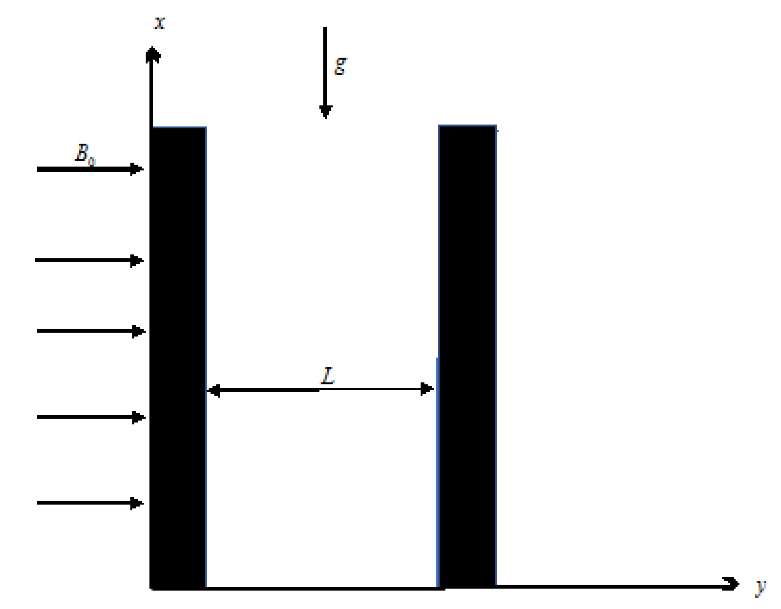
- (a)
- Microchannel length is infinite with width L;
- (b)
- The channel is along x-axis and normal to y-axis;
- (c)
- At t ≤ 0, the temperature of the system is ;
- (d)
- After t = , the temperature increases from to ;
- (e)
- Fluid accelerates in the x-direction;
- (f)
- The magnetic field of strength works transversely to the flow direction.
- The momentum equation
- The energy balance equation
- The generalized Fourier’s law for thermal flux
3. Solution of the Problem
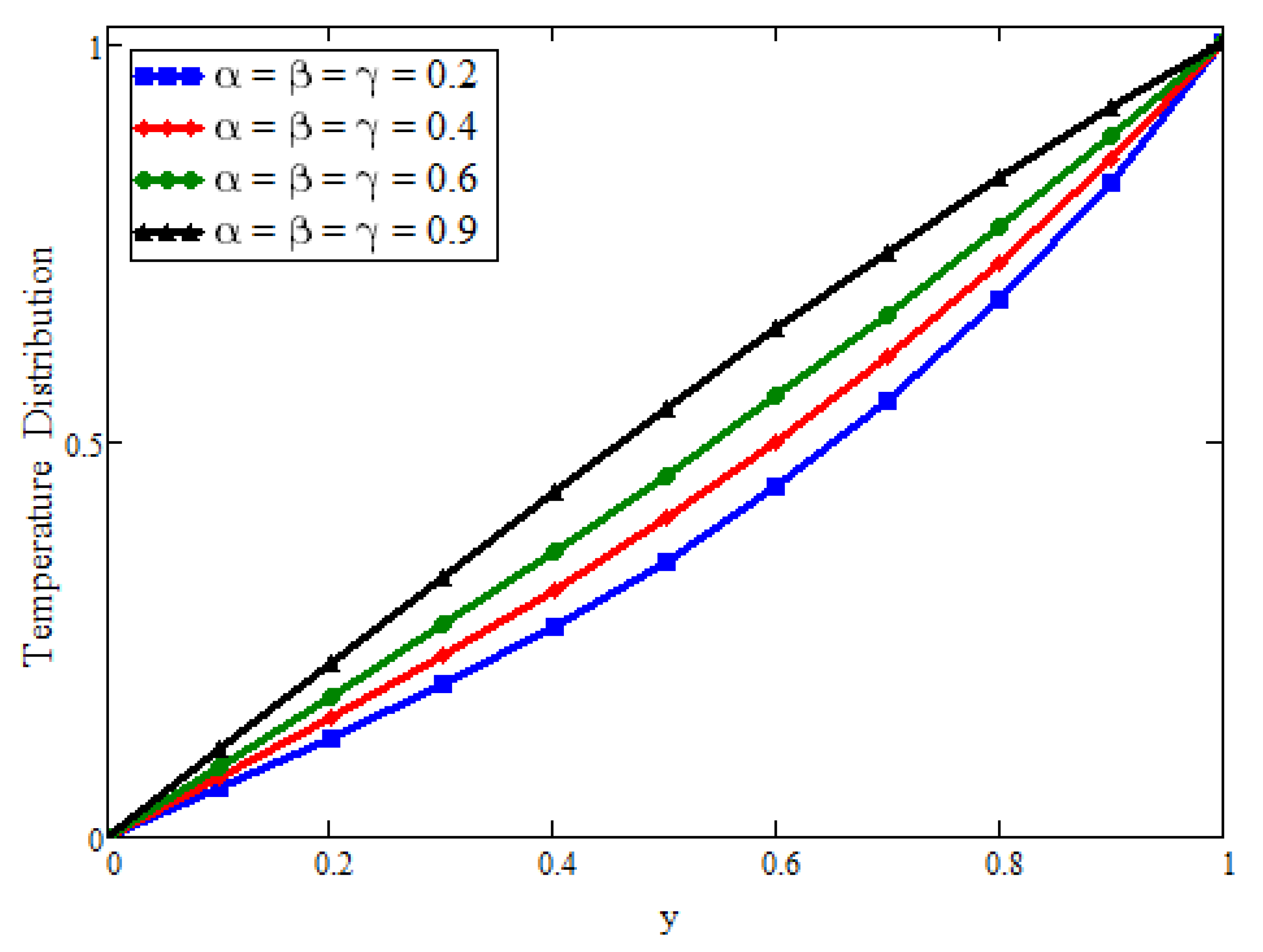
3.1. Temperature Field
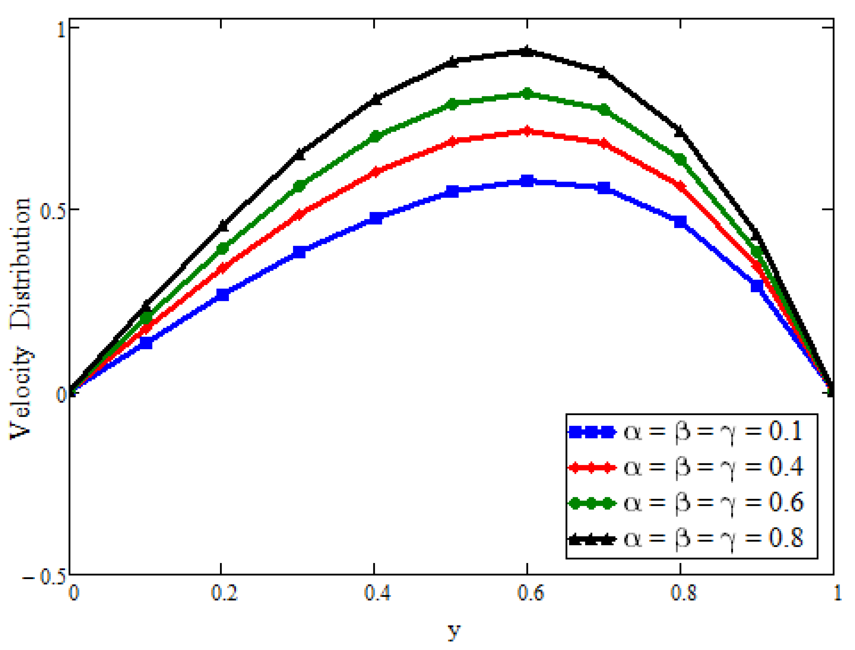
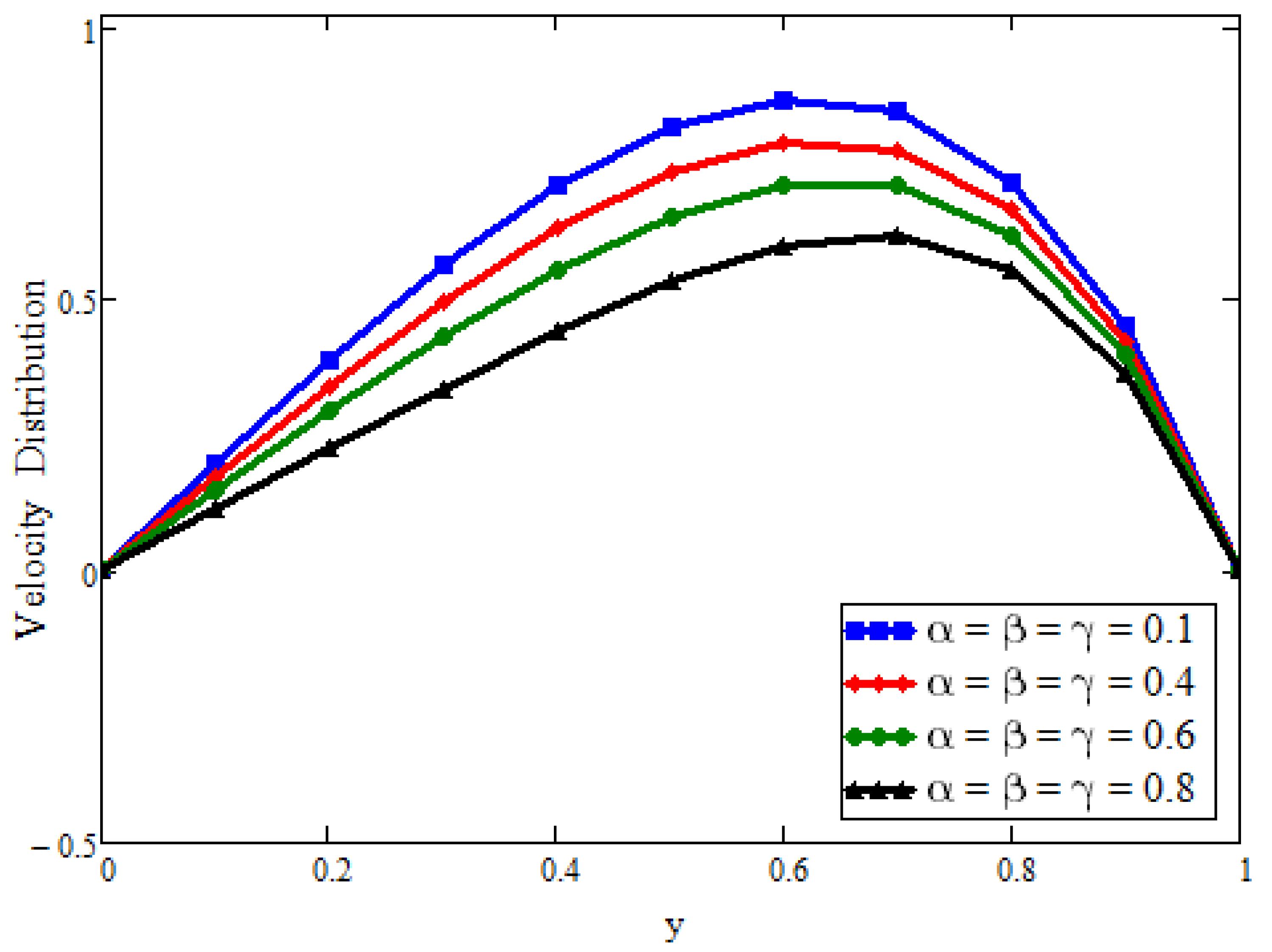
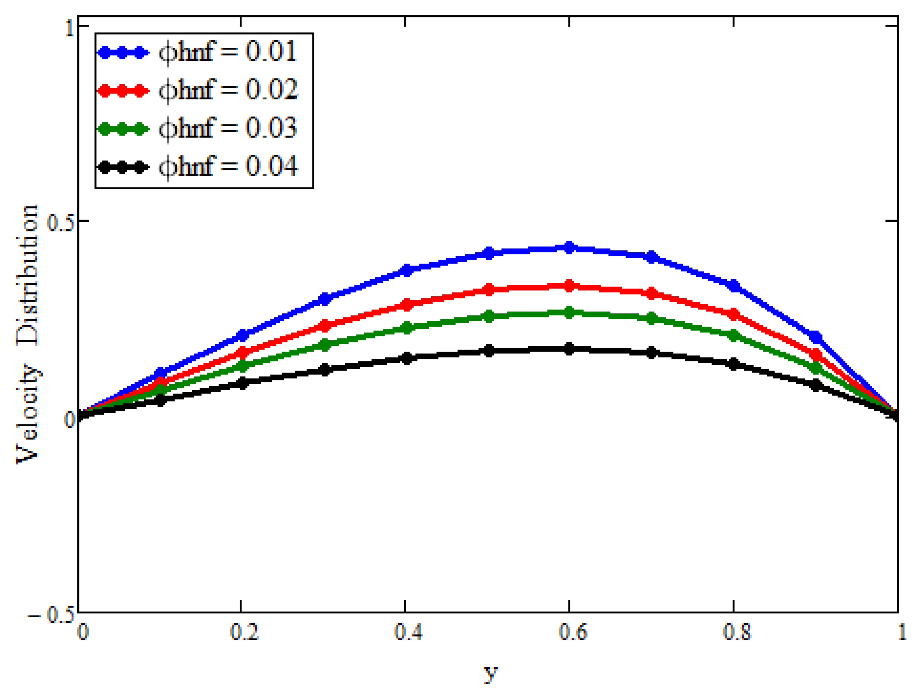
3.2. Velocity Field
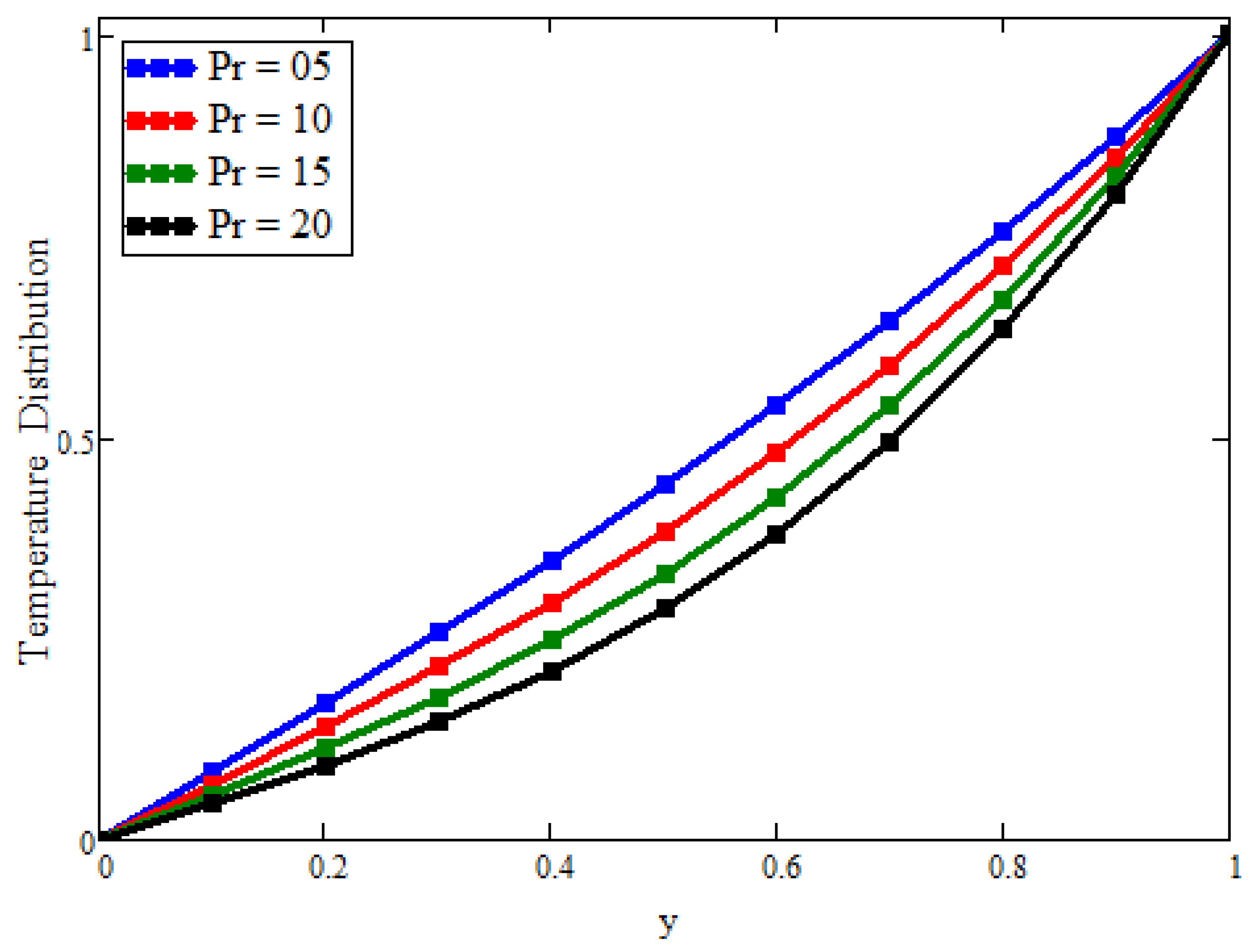
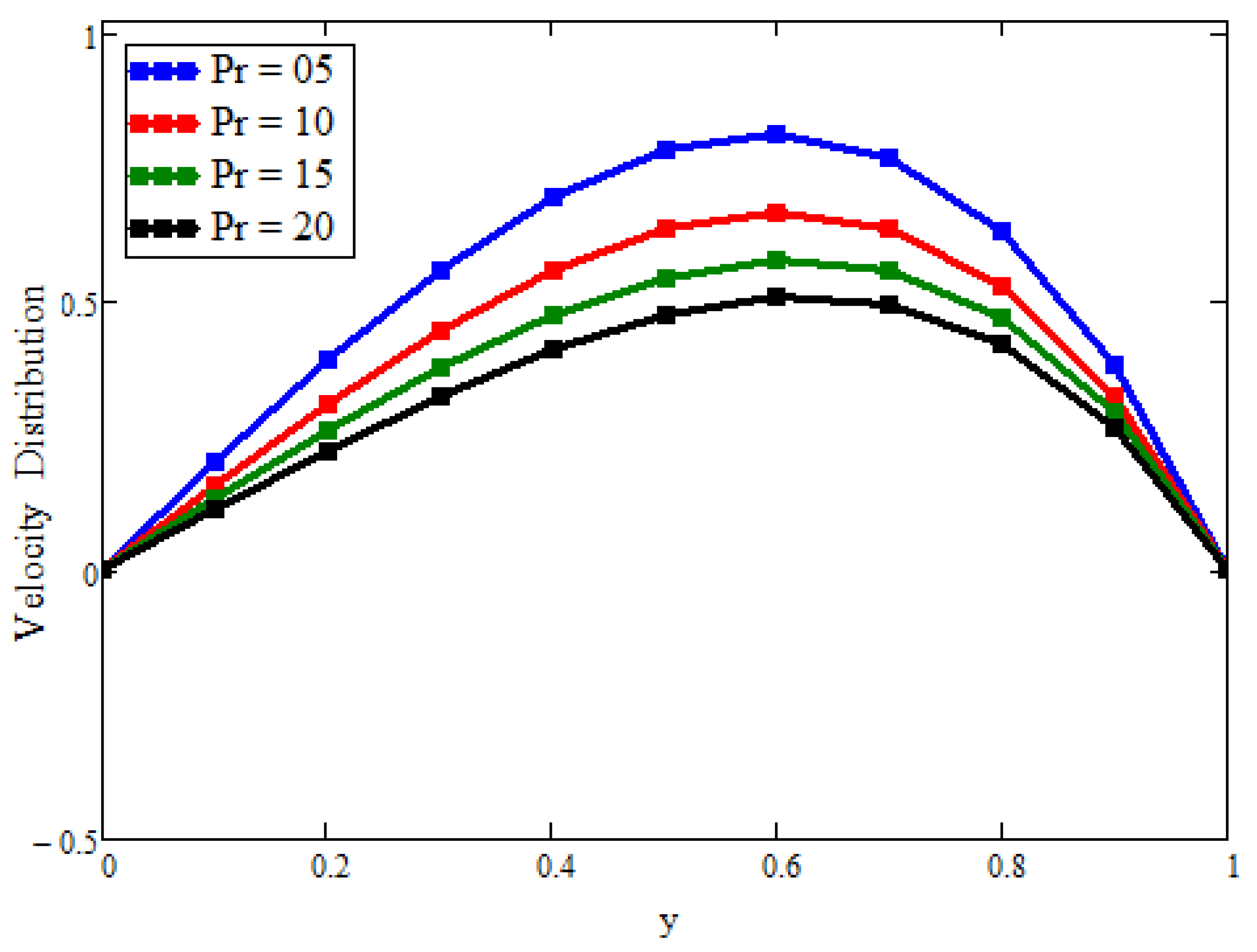
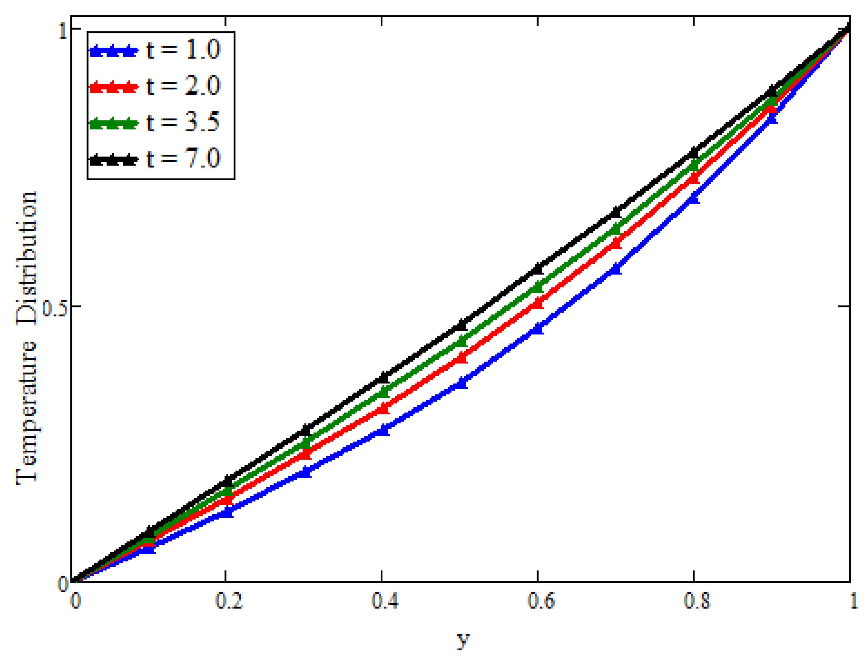
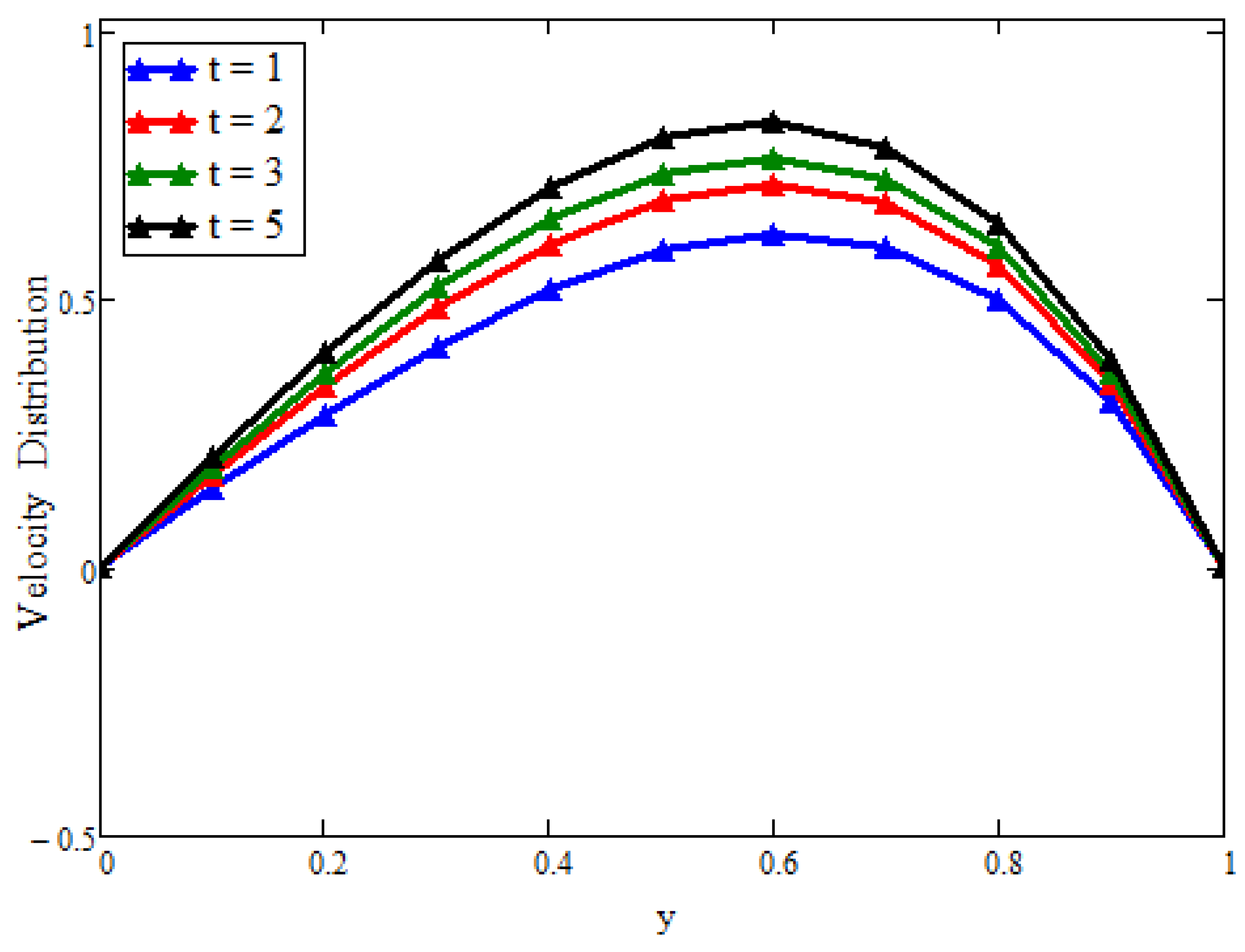
4. Discussion
5. Conclusions
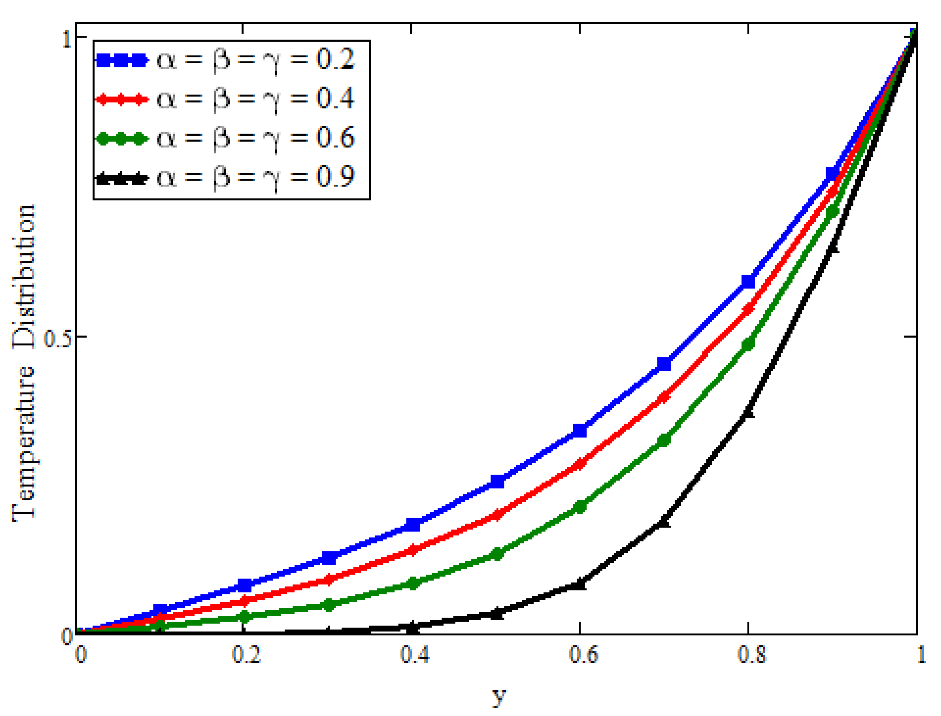
- Dual solutions for both temperature and velocity fields are predicted for different values of fractional parameters describing generalized. Fourier’s law (based on Prabhakar’s fractional derivative);
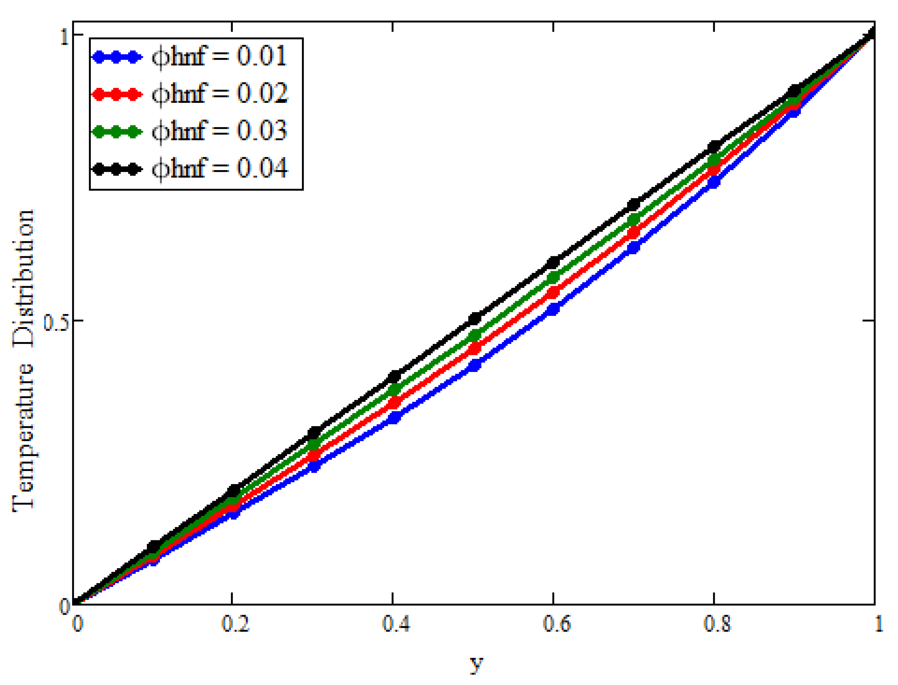
- Fluid property, i.e., temperature, can be enhanced by increasing the concentration level of nanoparticles;
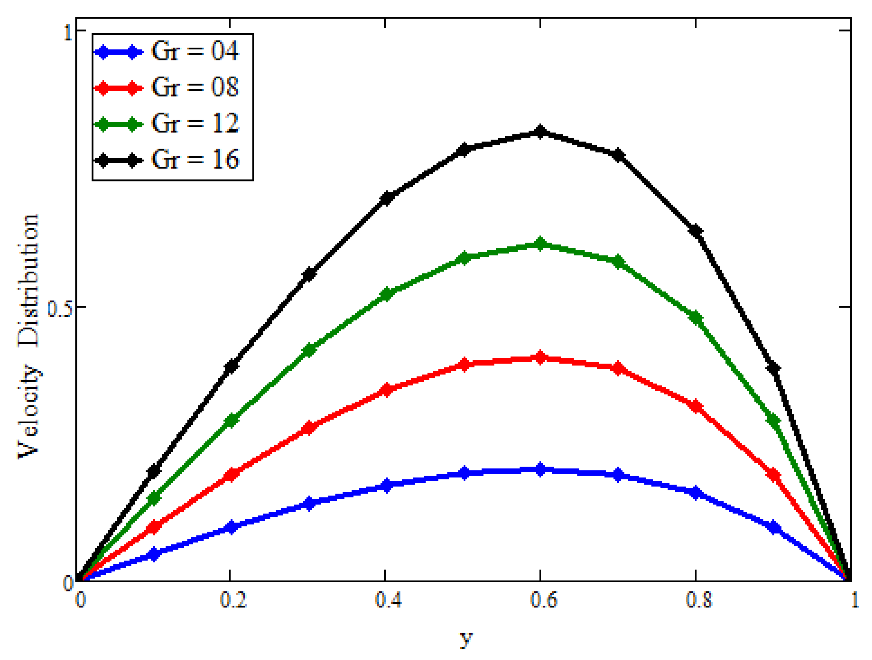
- Finally, the fractional parameters (which accomplish the heat memory impacts) can control the thermal and momentum boundary layer thickness;
- The obtained solutions can be beneficial for proper analysis of real data and provide a tool for testing possible approximate solutions where needed.
Author Contributions
Funding
Institutional Review Board Statement
Informed Consent Statement
Data Availability Statement
Acknowledgments
Conflicts of Interest
References
- Bräuer, F.; Trautner, E.; Hasslberger, J.; Cifani, P.; Klein, M. Turbulent Bubble-Laden Channel Flow of Power-Law Fluids: A Direct Numerical Simulation Study. Fluids 2021, 6, 40. [Google Scholar] [CrossRef]
- Zheng, Y.; Yang, H.; Mazaheri, H.; Aghaei, A.; Mokhtari, N.; Afrand, M. An investigation on the influence of the shape of the vortex generator on fluid flow and turbulent heat transfer of hybrid nanofluid in a channel. J. Therm. Anal. Calorim. 2021, 143, 1425–1438. [Google Scholar] [CrossRef]
- D’Ippolito, A.; Calomino, F.; Alfonsi, G.; Lauria, A. Flow Resistance in Open Channel Due to Vegetation at Reach Scale: A Review. Water 2021, 13, 116. [Google Scholar] [CrossRef]
- Choi, S.U.; Eastman, J.A. Enhancing Thermal Conductivity of Fluids with Nanoparticles (No. ANL/MSD/CP-84938.CONF-951135-29); Argonne National Lab.: Argonne, IL, USA, 1995. [Google Scholar]
- Nadeem, S.; Ahmad, S.; Khan, M.N. Mixed convection flow of hybrid nanoparticle along a Riga surface with Thomson and Troian slip condition. J. Therm. Anal. Calorim. 2021, 143, 2099–2109. [Google Scholar] [CrossRef]
- Reddy, M.G.; Shehzad, S.A. Molybdenum disulfide and magnesium oxide nanoparticle performance on micropolar Cattaneo-Christov heat flux model. Appl. Math. Mech. 2021, 42, 541–552. [Google Scholar] [CrossRef]
- Wole-Osho, I.; Okonkwo, E.C.; Adun, H.; Kavaz, D.; Abbasoglu, S. An intelligent approach to predicting the effect of nanoparticle mixture ratio, concentration and temperature on thermal conductivity of hybrid nanofluids. J. Therm. Anal. Calorim. 2021, 144, 671–688. [Google Scholar] [CrossRef] [Green Version]
- Haque, M.E.; Hossain, M.S.; Ali, H.M. Laminar forced convection heat transfer of nanofluids inside noncircular ducts: A review. Powder Technol. 2020. [Google Scholar] [CrossRef]
- Khashi’ie, N.S.; Arifin, N.M.; Pop, I.; Nazar, R. Melting heat transfer in hybrid nanofluid flow along a moving surface. J. Therm. Anal. Calorim. 2020. [Google Scholar] [CrossRef]
- Goldanlou, A.S.; Sepehrirad, M.; Papi, M.; Hussein, A.K.; Afrand, M.; Rostami, S. Heat transfer of hybrid nanofluid in a shell and tube heat exchanger equipped with blade-shape turbulators. J. Therm. Anal. Calorim. 2021, 143, 1689–1700. [Google Scholar] [CrossRef]
- Montazer, E.; Shafii, M.B.; Salami, E.; Muhamad, M.R.; Yarmand, H.; Gharehkhani, S.; Badarudin, A. Heat transfer in turbulent nanofluids: Separation flow studies and development of novel correlations. Adv. Powder Technol. 2020, 31, 3120–3133. [Google Scholar] [CrossRef]
- Benkhedda, M.; Boufendi, T.; Tayebi, T.; Chamkha, A.J. Convective heat transfer performance of hybrid nanofluid in a horizontal pipe considering nanoparticles shapes effect. J. Therm. Anal. Calorim. 2020, 140, 411–425. [Google Scholar] [CrossRef]
- Bhattad, A.; Sarkar, J.; Ghosh, P. Hydrothermal performance of different alumina hybrid nanofluid types in plate heat exchanger. J. Therm. Anal. Calorim. 2020, 139, 3777–3787. [Google Scholar] [CrossRef]
- Izadi, M. Effects of porous material on transient natural convection heat transfer of nanofluids inside a triangular chamber. Chin. J. Chem. Eng. 2020, 28, 1203–1213. [Google Scholar] [CrossRef]
- Waini, I.; Ishak, A.; Groşan, T.; Pop, I. Mixed convection of a hybrid nanofluid flow along a vertical surface embedded in a porous medium. Int. Commun. Heat Mass Transf. 2020, 114, 104565. [Google Scholar] [CrossRef]
- Pandya, N.S.; Desai, A.N.; Tiwari, A.K.; Said, Z. Influence of the geometrical parameters and particle concentration levels of hybrid nanofluid on the thermal performance of axial grooved heat pipe. Therm. Sci. Eng. Prog. 2021, 21, 100762. [Google Scholar] [CrossRef]
- Babazadeh, H.; Shah, Z.; Ullah, I.; Kumam, P.; Shafee, A. Analysis of hybrid nanofluid behavior within a porous cavity including Lorentz forces and radiation impacts. J. Therm. Anal. Calorim. 2021, 143, 1129–1137. [Google Scholar] [CrossRef]
- Asadi, A.; Alarifi, I.M.; Foong, L.K. An experimental study on characterization, stability and dynamic viscosity of CuO-TiO2/water hybrid nanofluid. J. Mol. Liq. 2020, 307, 112987. [Google Scholar] [CrossRef]
- Ikram, M.D.; Asjad, M.; Ahmadian, A.; Ferrara, M. A new fractional mathematical model of extraction nanofluids using clay nanoparticles for different based fluids. Math. Methods Appl. Sci. 2020. [Google Scholar] [CrossRef]
- Huminic, G.; Huminic, A. Entropy generation of nanofluid and hybrid nanofluid flow in thermal systems: A review. J. Mol. Liq. 2020, 302, 112533. [Google Scholar] [CrossRef]
- Nadeem, S.; Abbas, N.; Malik, M.Y. Inspection of hybrid based nanofluid flow over a curved surface. Comput. Methods Programs Biomed. 2020, 189, 105193. [Google Scholar] [CrossRef]
- Baleanu, D.; Diethelm, K.; Scalas, E.; Trujillo, J.J. Fractional Calculus: Models and Numerical Methods; World Scientific: London, UK, 2012; Volume 3. [Google Scholar]
- Ortigueira, M.D.; Machado, J.T. Fractional derivatives: The perspective of system theory. Mathematics 2019, 7, 150. [Google Scholar] [CrossRef] [Green Version]
- Sene, N. Second-grade fluid model with Caputo–Liouville generalised fractional derivative. Chaos Solitons Fractals 2020, 133, 109631. [Google Scholar] [CrossRef]
- Mozafarifard, M.; Toghraie, D. Time-fractional subdiffusion model for thin metal films under femtosecond laser pulses based on Caputo fractional derivative to examine anomalous diffusion process. Int. J. Heat Mass Transf. 2020, 153, 119592. [Google Scholar] [CrossRef]
- Thabet, S.T.; Abdo, M.S.; Shah, K.; Abdeljawad, T. Study of transmission dynamics of COVID-19 mathematical model under ABC fractional order derivative. Results Phys. 2020, 19, 103507. [Google Scholar] [CrossRef]
- Prabhakar, T.R. A Singular Integral Equation with a Generalized Mittag Leffler Function in the Kernel. 1971. Available online: https://www.semanticscholar.org/paper/A-SINGULAR-INTEGRAL-EQUATION-WITH-A-GENERALIZED-IN-Prabhakar/cf26590a6a758228228045275591231430db614f (accessed on 2 July 2021).
- Yang, X.J. General Fractional Derivatives: Theory, Methods and Applications; CRC Press: Boca Raton, FL, USA, 2019. [Google Scholar]
- Garra, R.; Gorenflo, R.; Polito, F.; Tomovski, Ž. Hilfer–Prabhakar derivatives and some applications. Appl. Math. Comput. 2014, 242, 576–589. [Google Scholar] [CrossRef] [Green Version]
- Fernandez, A.; Baleanu, D. Classes of operators in fractional calculus: A case study. Math. Methods Appl. Sci. 2021. [Google Scholar] [CrossRef]
- Giusti, A.; Colombaro, I. Prabhakar-like fractional viscoelasticity. Commun. Nonlinear Sci. Numer. Simul. 2018, 56, 138–143. [Google Scholar] [CrossRef] [Green Version]
- Elnaqeeb, T.; Shah, N.A.; Mirza, I.A. Natural convection flows of carbon nanotubes nanofluids with Prabhakar-like thermal transport. Math. Methods Appl. Sci. 2020. [Google Scholar] [CrossRef]
- Shah, N.A.; Fetecau, C.; Vieru, D. Natural convection flows of Prabhakar-like fractional Maxwell fluids with generalized thermal transport. J. Therm. Anal. Calorim. 2021, 143, 2245–2258. [Google Scholar] [CrossRef]
- Akgül, A.; Siddique, I. Novel applications of the magnetohydrodynamics couple stress fluid flows between two plates with fractal-fractional derivatives. Numer. Methods Part. Differ. Equ. 2021, 37, 2178–2189. [Google Scholar] [CrossRef]
- Wang, F.; Asjad, M.I.; Zahid, M.; Iqbal, A.; Ahmad, H.; Alsulami, M.D. Unsteady thermal transport flow of Casson nanofluids with generalized Mittag-Leffler kernel of Prabhakar’s type. J. Mater. Res. Technol. 2021. [Google Scholar] [CrossRef]
- Tashtoush, B.; Magableh, A. Magnetic field effect on heat transfer and fluid flow characteristics of blood flow in multi-stenosis arteries. Heat Mass Transf. 2008, 44, 297–304. [Google Scholar] [CrossRef]
- Saqib, M.; Shafie, S.; Khan, I.; Chu, Y.M.; Nisar, K.S. Symmetric MHD channel flow of nonlocal fractional model of BTF containing hybrid nanoparticles. Symmetry 2020, 12, 663. [Google Scholar] [CrossRef]
- Polito, F.; Tomovski, Z. Some properties of Prabhakar-type fractional calculus operators. Fract. Differ. Calc. 2016, 6, 73–94. [Google Scholar] [CrossRef]


| Nanofluid | Hybrid Nanofluid |
|---|---|
Publisher’s Note: MDPI stays neutral with regard to jurisdictional claims in published maps and institutional affiliations. |
© 2021 by the authors. Licensee MDPI, Basel, Switzerland. This article is an open access article distributed under the terms and conditions of the Creative Commons Attribution (CC BY) license (https://creativecommons.org/licenses/by/4.0/).
Share and Cite
Asjad, M.I.; Sarwar, N.; Hafeez, M.B.; Sumelka, W.; Muhammad, T. Advancement of Non-Newtonian Fluid with Hybrid Nanoparticles in a Convective Channel and Prabhakar’s Fractional Derivative—Analytical Solution. Fractal Fract. 2021, 5, 99. https://doi.org/10.3390/fractalfract5030099
Asjad MI, Sarwar N, Hafeez MB, Sumelka W, Muhammad T. Advancement of Non-Newtonian Fluid with Hybrid Nanoparticles in a Convective Channel and Prabhakar’s Fractional Derivative—Analytical Solution. Fractal and Fractional. 2021; 5(3):99. https://doi.org/10.3390/fractalfract5030099
Chicago/Turabian StyleAsjad, Muhammad Imran, Noman Sarwar, Muhammad Bilal Hafeez, Wojciech Sumelka, and Taseer Muhammad. 2021. "Advancement of Non-Newtonian Fluid with Hybrid Nanoparticles in a Convective Channel and Prabhakar’s Fractional Derivative—Analytical Solution" Fractal and Fractional 5, no. 3: 99. https://doi.org/10.3390/fractalfract5030099
APA StyleAsjad, M. I., Sarwar, N., Hafeez, M. B., Sumelka, W., & Muhammad, T. (2021). Advancement of Non-Newtonian Fluid with Hybrid Nanoparticles in a Convective Channel and Prabhakar’s Fractional Derivative—Analytical Solution. Fractal and Fractional, 5(3), 99. https://doi.org/10.3390/fractalfract5030099