
Particularities of Forest Dynamics Using Higuchi Dimension. Parâng Mountains as a Case Study


 , , ,
, , , 
Abstract
:1. Introduction
2. Materials
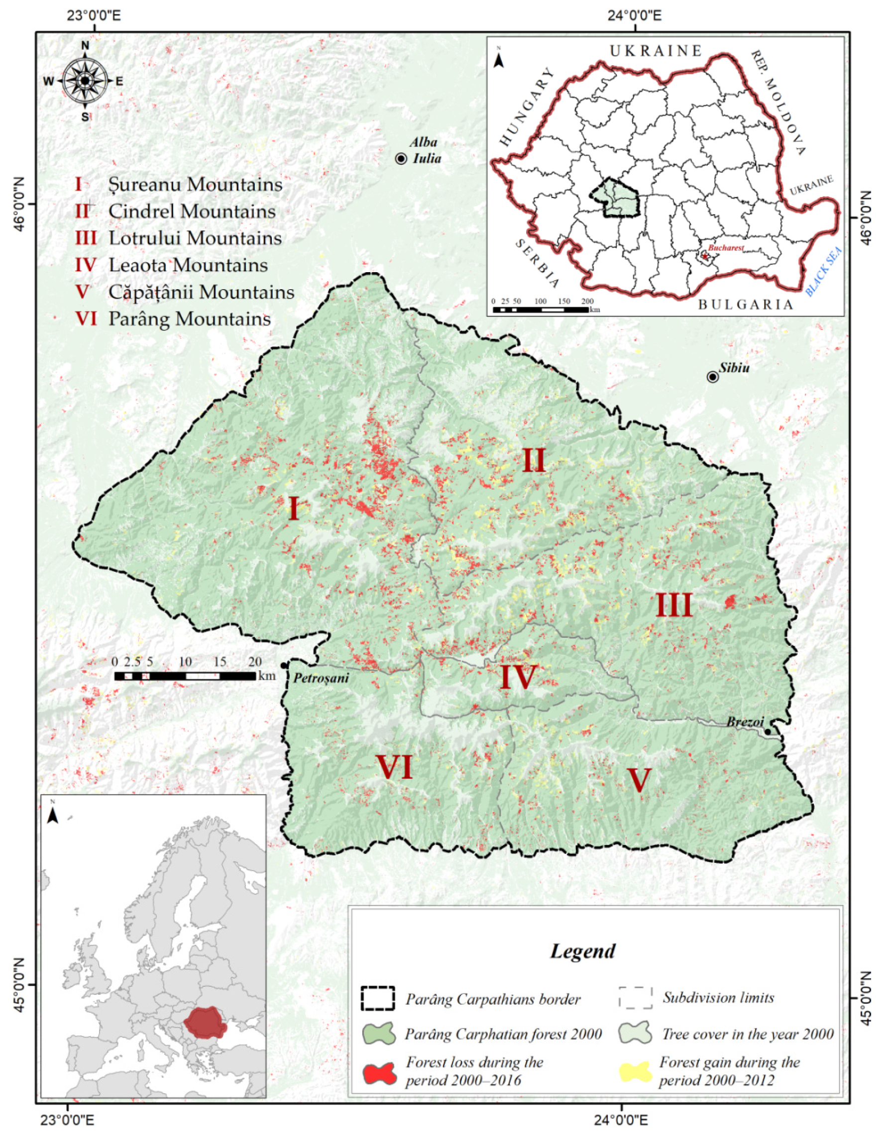
2.1. Study Area
2.2. Data and Image Processing
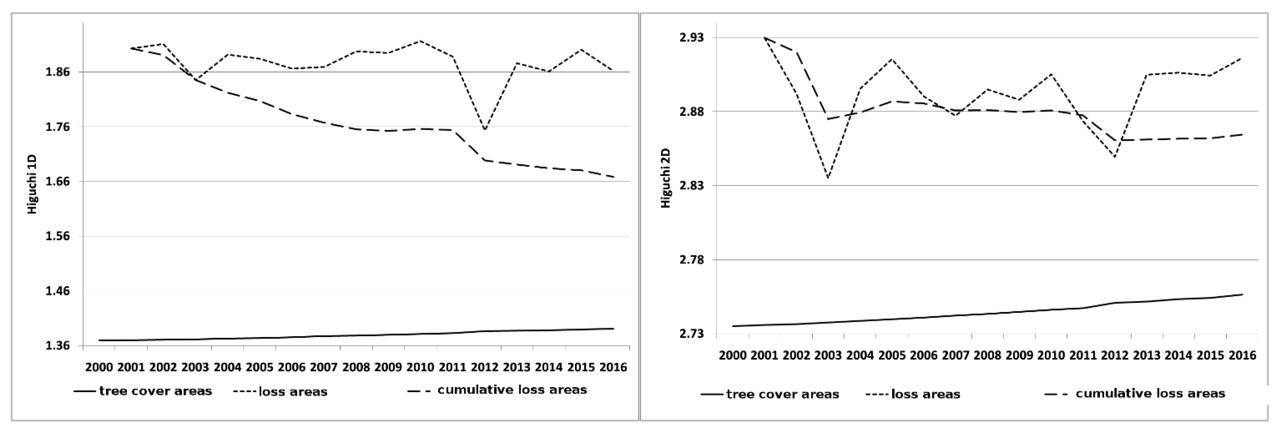
2.3. Higuchi 1D
2.4. Higuchi 2D
2.5. Statistics
3. Results and Discussion
4. Discussion
5. Conclusions
Author Contributions
Funding
Institutional Review Board Statement
Informed Consent Statement
Data Availability Statement
Acknowledgments
Conflicts of Interest
References
- Stickler, C.M.; Nepstad, D.C.; Coe, M.T.; McGrath, D.G.; Rodrigues, H.O.; Walker, W.S.; Soares-Filho, B.S.; Davidson, E.A. The potential ecological costs and cobenefits of REDD: A critical review and case study from the Amazon region. Glob. Chang. Biol. 2019, 15, 2803–2824. [Google Scholar] [CrossRef]
- Fraser, E.D.G.; Stringer, L.C. Explaining agricultural collapse: Macro-forces, micro-crises and the emergence of land use vulnerability in southern Romania. Glob. Environ. Chang. 2009, 19, 45–53. [Google Scholar] [CrossRef]
- Keenan, R.; Reams, G.; Freitas, J.; Lindquist, E.; Achard, F.; Grainger, A. Dynamics of global forest area: Results from the 2015 Global Forest Resources Assessment. For. Ecol. Manag. 2015, 352, 9–20. [Google Scholar] [CrossRef]
- Lawrence, D.; Vandecar, K. Effects of tropical deforestation on climate and agriculture. Nat. Clim. Chang. 2015, 5, 27–36. [Google Scholar] [CrossRef]
- Pintilii, R.D.; Papuc, R.M.; Draghici, C.C.; Simion, A.G.; Ciobotaru, A.M. The impact of deforestation on the structural dynamics of economic profile in the most affected territorial systems in Romania. In Proceedings of the 15th International Multidisciplinary Scientific Geoconference (SGEM), Albena, Bulgaria, 18–24 June 2015; Volume 3, pp. 567–573. [Google Scholar] [CrossRef]
- Pintilii, R.D.; Andronache, I.; Diaconu, D.C.; Dobrea, R.C.; Zelenakova, M.; Fensholt, R.; Peptenatu, D.; Draghici, C.C.; Ciobotaru, A.M. Using Fractal Analysis in Modeling the Dynamics of Forest and Economic Impact Assessment: Maramureș County, Romania, as a Case Study. Forests 2017, 8, 25. [Google Scholar] [CrossRef] [Green Version]
- Peptenatu, D.; Sirodoev, I.; Pravalie, R. Quantification of the aridity process in south-western Romania. J. Environ. Health Sci. Eng. 2013, 11, 5. [Google Scholar] [CrossRef] [PubMed] [Green Version]
- FAO. The State of Food and Agriculture. Innovation in Family Farming, Food and Agriculture; FAO: Rome, Italy, 2014; Available online: http://www.fao.org/3/a-i4040e.pdf (accessed on 21 December 2017).
- United Nations. Deforestation Slows, ‘but We Need to Do Better’ on Sustainable Forest Use—UN Agriculture Chief. Available online: http://www.un.org/apps/news/story.asp?NewsID=51814#.WLGdPFV97Dc (accessed on 11 February 2018).
- Griffiths, P.; Kuemmerle, T.; Baumann, M.; Radeloff, V.C.; Abrudan, I.V.; Lieskovsky, J.; Munteanu, C.; Ostapowicz, K.; Hostert, P. Forest disturbance, forest recovery., and changes in forest types across the Carpathian ecoregion from 1985 to 2010 based on Landsat image composites. Remote. Sens. Environ. 2013, 151, 72–88. [Google Scholar] [CrossRef]
- Hostert, P.; Kuemmerle, T.; Prishchepov, A.; Sieber, A.; Lambin, E.F.; Radeloff, V.C. Rapid land use change after socio-economic disturbances: The collapse of the Soviet Union versus Chernobyl. Environ. Res. Lett. 2011, 6, 045201. [Google Scholar] [CrossRef]
- Knorn, J.; Kuemmerle, T.; Radeloff, V.C.; Szabo, A.; Mindrescu, M.; Keeton, W.S. Forest restitution and protected area effectiveness in post-socialist Romania. Biol. Conserv. 2012, 146, 204–212. [Google Scholar] [CrossRef]
- Kummerle, T.; Chaskovskyy, O.; Knorn, J.; Radeloff, V.C.; Kruhlov, I.; Keeton, W.S.; Hostert, P. Forest cover change and illegal logging in the Ukrainian Carpathians in the transition period from 1988 to 2007. Remote. Sens. Environ. 2009, 113, 1194–1207. [Google Scholar] [CrossRef]
- Kummerle, T.; Muller, D.; Griffiths, P.; Rusu, M. Land use change in Southern Romania after the collapse of socialism. Reg. Environ. Change 2008, 9, 1–12. [Google Scholar] [CrossRef]
- FAO. State of the World’s Forests. Forest and Agriculture: Land-Use Challenge and Opportunities; FAO: Rome, Italy, 2014; Available online: http://www.fao.org/3/a-i5588e.pdf (accessed on 22 December 2017).
- Andersson, F.; Birot, Y.; Paivinen, R. Towards the Sustainable Use of Europe’s Forests—Forest Ecosystem and Landscape Research: Scientific Challenges and Opportunities. In Proceedings 49 of European Forest Institute, Joensuu, Finland; European Forest Institute: Joensuu, Finland, 2004. [Google Scholar]
- Andronache, I.; Fensholt, R.; Ahammer, H.; Ciobotaru, A.M.; Pintilii, R.D.; Peptenatu, D.; Draghici, C.C.; Diaconu, D.C.; Radulovic, M.; Pulighe, G.; et al. Assessment of Textural Differentiations in Forest Resources in Romania Using Fractal Analysis. Forests 2017, 8, 54. [Google Scholar] [CrossRef] [Green Version]
- Guvernul României—Ministerul Mediului și Schimbărilor Climatice. Arii Naturale Protejate. 2017. Available online: http://www.mmediu.ro/beta/domenii/protectia-naturii-2/arii-naturale-protejate/ (accessed on 12 December 2017).
- Pintilii, R.D.; Andronache, I.; Simion, A.G.; Draghici, C.C.; Peptenatu, D.; Ciobotaru, A.M.; Dobrea, R.C.; Papuc, R.M. Determining forest fund evolution by fractal analysis (Suceava-Romania). Urban. Archit. Constr. 2016, 7, 31–42. [Google Scholar]
- Marinescu, E.; Marinescu, E.I.; Vladut, A.; Marinescu, S. Forest Cover Change in the Parâng-Cindrel Mountains of the Southern Carpathians, Romania; Springer: Berlin/Heidelberg, Germany, 2013; pp. 225–238. [Google Scholar] [CrossRef]
- Hansen, M.C.; Potapov, P.V.; Moore, R.; Hancher, M.; Turubanova, S.A.; Tyukavina, A.; Thau, D.; Stehman, S.V.; Goetz, S.J.; Loveland, T.R.; et al. High-Resolution Global Maps of 21st-Century Forest Cover Change. Science 2013, 342, 850–853. [Google Scholar] [CrossRef] [Green Version]
- McGarigal, K.S.; Cushman, S.A. Surface metrics: An alternative to patch metrics for the quantification of landscape structure. Landsc. Ecol. 2009, 24, 433–450. [Google Scholar] [CrossRef]
- Kedron, P.J.; Frazier, A.E.; Ovando-Montejo, G.A.; Wang, J. Surface metrics for landscape ecology: A comparison of landscape models across ecoregions and scales. Landsc. Ecol. 2018, 33, 1489–1504. [Google Scholar] [CrossRef]
- Calabrese, J.M.; Fagan, W.F. A comparison-shopper’s guide to connectivity metrics. Front. Ecol. Environ. 2004, 2, 529–536. [Google Scholar] [CrossRef]
- Sellan, G.; Simini, F.; Maritan, A.; Banavar, J.R.; de Haulleville, T.; Bauters, M.; Anfodillo, T. Testing a general approach to assess the degree of disturbance in tropical forests. J. Veg. Sci. 2017, 28, 659–668. [Google Scholar] [CrossRef] [Green Version]
- Stauffer, D.; Aharony, A. Introduction to Percolation Theory; Taylor & Francis: London, UK, 1992; 192p. [Google Scholar] [CrossRef]
- McGarigal, K.; Marks, B.J. FRAGSTATS: Spatial Analysis Program for Quantifying Landscape Structure. USDA Forest Service General Technical Report PNW-GTR-351; U.S. Department of Agriculture: Portland, OR, USA, 1995; 122p. [CrossRef]
- Romero, S.; Campbell, J.F.; Nechols, J.R.; With, K.A. Movement behavior in response to landscape structure: Role of functional grain. Landsc. Ecol. 2009, 24, 39–51. [Google Scholar] [CrossRef]
- Riitters, K.; Wickham, J. Decline of forest interior conditions in the conterminous United States. Sci. Rep. 2012, 2, 653. [Google Scholar] [CrossRef] [PubMed] [Green Version]
- O’Neill, R.V.; Krummel, J.; Gardner, R.H.; Sugihara, G.; Jackson, B.; DeAngelis, D.L.; Dale, V.H. Indices of landscape pattern. Landsc. Ecol. 1988, 1, 153–162. [Google Scholar] [CrossRef]
- Li, H.; Reynolds, J.F. A new contagion index to quantify spatial patterns of landscapes. Landsc. Ecol. 1993, 8, 155–162. [Google Scholar] [CrossRef]
- Legendre, P.; Fortin, M.J. Spatial pattern and ecological analysis. Vegetatio 1989, 80, 107. [Google Scholar] [CrossRef]
- Gustafson, E.J.; Parker, G.R. Relationships between landcover proportion and indexes of landscape spatial pattern. Landsc. Ecol. 1992, 7, 101–110. [Google Scholar] [CrossRef]
- Higuchi, T. Approach to an irregular time series on the basis of the fractal theory. Phys. D Nonlinear Phenom. 1988, 31, 277–283. [Google Scholar] [CrossRef]
- Ahammer, H. Higuchi Dimension of Digital Images. PLoS ONE 2011, 6, e24796. [Google Scholar] [CrossRef]
- Andronache, I.; Ahammer, H.; Jelinek, H.F.; Peptenatu, D.; Ciobotaru, A.M.; Draghici, C.C.; Pintilii, R.D.; Simion, A.G.; Teodorescu, C. Fractal analysis for studying the evolution of forests. Chaos Solitons Fractals 2016, 91, 310–318. [Google Scholar] [CrossRef]
- Spasic, S. On 2D generalization of Higuchi’s fractal dimension. Chaos Solitons Fractals 2014, 69, 179–187. [Google Scholar] [CrossRef]
- Ahammer, H.; Sabathiel, N.; Reiss, M.A. Is a two-dimensional generalization of the Higuchi algorithm really necessary? Chaos Solitons Fractals 2015, 25, 073104. [Google Scholar] [CrossRef]
- Kainz, P.; Mayrhofer-Reinhartshuber, M.; Ahammer, H. IQM: An Extensible and Portable Open Source Application for Image and Signal Analysis in Java. PLoS ONE 2015, 10, e0116329. [Google Scholar] [CrossRef] [PubMed] [Green Version]
- Concezzi, M.; Spigler, R. An ADI Method for the Numerical Solution of 3D Fractional Reaction-Diffusion Equations. Fractal Fract. 2020, 4, 57. [Google Scholar] [CrossRef]
- Di Ieva, A.; Grizzi, F.; Jelinek, H.F.; Pellionisz, A.J.; Losa, G.A. Fractals in the neurosciences, Part I: General principles and basic neurosciences. Neuroscientist 2013, 20, 403–417. [Google Scholar] [CrossRef]
- Sarkar, N.; Chaudhuri, B. An efficient differential box-counting approach to compute fractal dimension of image. IEEE Trans. Syst. Man Cybern. 1994, 24, 115–120. [Google Scholar] [CrossRef] [Green Version]
- Jelinek, H.F.; Ahammer, H.; Matthews, S.; Succar, P.; McLachlan, C.; Buckl, M. Establishing a reference range for oligodendroglioma classification using Higuchi dimension analysis. In Proceedings of the 9th IASTED International Conference on Biomedical Engineering, BioMed, Innsbruck, Austria, 28 February 2012; pp. 25–28. [Google Scholar] [CrossRef]
- Halley, J.M.; Hartley, S.; Kallimanis, A.S.; Kunin, W.E.; Lennon, J.J.; Sgardelis, S.P. Uses and abuses of fractal methodology in ecology. Ecol. Lett. 2004, 7, 254–271. [Google Scholar] [CrossRef]
- He, H.S.; DeZonia, B.E.; Mladenoff, D.J. An aggregation index (AI) to quantify spatial patterns of landscapes. Landsc. Ecol. 2000, 15, 591–601. [Google Scholar] [CrossRef]
- Landini, G. Fractals in microscopy. J. Microsc. 2011, 241, 1–8. [Google Scholar] [CrossRef]
- Phan, D.T.H.; Brouwer, R.; Davidson, M. The economic costs of avoided deforestation in the developing world: A meta-analysis. J. For. Econ. 2014, 20, 1–16. [Google Scholar] [CrossRef]
- Parks, N. Deforestation-related climate impacts may vary by soil. Front. Ecol. Environ. 2014, 12, 204. [Google Scholar]
- Botsch, J.C.; Walter, S.T.; Karubian, J.; Gonzalez, N.; Dobbs, E.K.; Brosi, B.J. Impacts of forest fragmentation on orchid bee (Hymenoptera: Apidae: Euglossini) communities in the Choc biodiversity hotspot of northwest Ecuador. J. Insect Conserv. 2017, 21, 633–643. [Google Scholar] [CrossRef]
- Peptenatu, D.; Merciu, C.; Merciu, G.; Draghici, C.C.; Cercleux, L. Specific features of environment risk management in emerging territorial Structures. Carpathian J. Earth Environ. Sci. 2012, 7, 135–143. [Google Scholar]
- Ciobotaru, A.M.; Peptenatu, D.; Andronache, I.; Simion, A.G. Fractal characteristics of the afforested, deforested and regenerated areas in Suceava County, Romania. In Proceedings of the International Scientific Conferences on Earth&Geo Sciences—SGEM Vienna Green Sessions 2016, Vienna, Austria, 2–5 November 2016; Stef92 Technology Ltd.: Sofia, Bulgaria, 2016; pp. 445–452. [Google Scholar]
- Pravalie, R.; Sirodoev, I.; Patriche, C.V.; Bandoc, G.; Peptenatu, D. The analysis of the relationship between climatic water deficit and corn agricultural productivity in the Dobrogea plateau. Carpathian J. Earth Environ. Sci. 2014, 9, 201–214. [Google Scholar]
- Pravalie, R.; Sîrdoev, I.; Peptenatu, D. Changes in the forest ecosystems in areas impacted by aridization in south-western Romania. Iran. J. Environ. Health Sci. Eng. 2014, 12, 2. [Google Scholar] [CrossRef] [Green Version]
- Pravalie, R.; Patriche, C.V.; Sirodoev, I.; Bandoc, G.; Dumitrescu, M.; Peptenatu, D. Water deficit and corn productivity during the post-socialist period. Case study: Southern Oltenia drylands, Romania. Arid. Land Res. Manag. 2016, 30, 239–257. [Google Scholar] [CrossRef]
- Braghină, C.; Peptenatu, D.; Draghici, C.C.; Pintilii, R.D.; Schvab, A. Territorial Management within the Systems Affected by Mining. Case study The South-Western Development region in Romania. Iran. J. Environ. Health Sci. Eng. 2011, 8, 343–352. [Google Scholar]
- Diaconu, D.C.; Peptenatu, D.; Simion, A.G.; Pintilii, R.D.; Draghici, C.C.; Teodorescu, C.; Grecu, A.; Gruia, A.K.; Ilie, A.M. The restrictions imposed upon the urban development by the piezometric level. Case study: Otopeni-Tunari, Corbeanca. Urban. Arhit. Constr. 2017, 8, 27–36. [Google Scholar]
- Draghici, C.C.; Peptenatu, D.; Simion, A.G.; Pintilii, R.D.; Diaconu, D.C.; Teodorescu, C.; Papuc, R.M.; Grigore, A.M.; Dobrea, C.R. Assessing economic pressure on the forest fund of Maramures County Romania. J. For. Sci. 2016, 62, 175–185. [Google Scholar] [CrossRef] [Green Version]
- Draghici, C.C.; Andronache, I.; Ahammer, H.; Peptenatu, D.; Pintilii, R.D.; Ciobotaru, A.M.; Simion, A.G.; Dobrea, R.C.; Diaconu, D.C.; Vişan, M.C.; et al. Spatial evolution of forest areas in the Northern Carpathian Mountains of Romania. Acta Montan. Slovaca 2017, 22, 95–106. [Google Scholar]


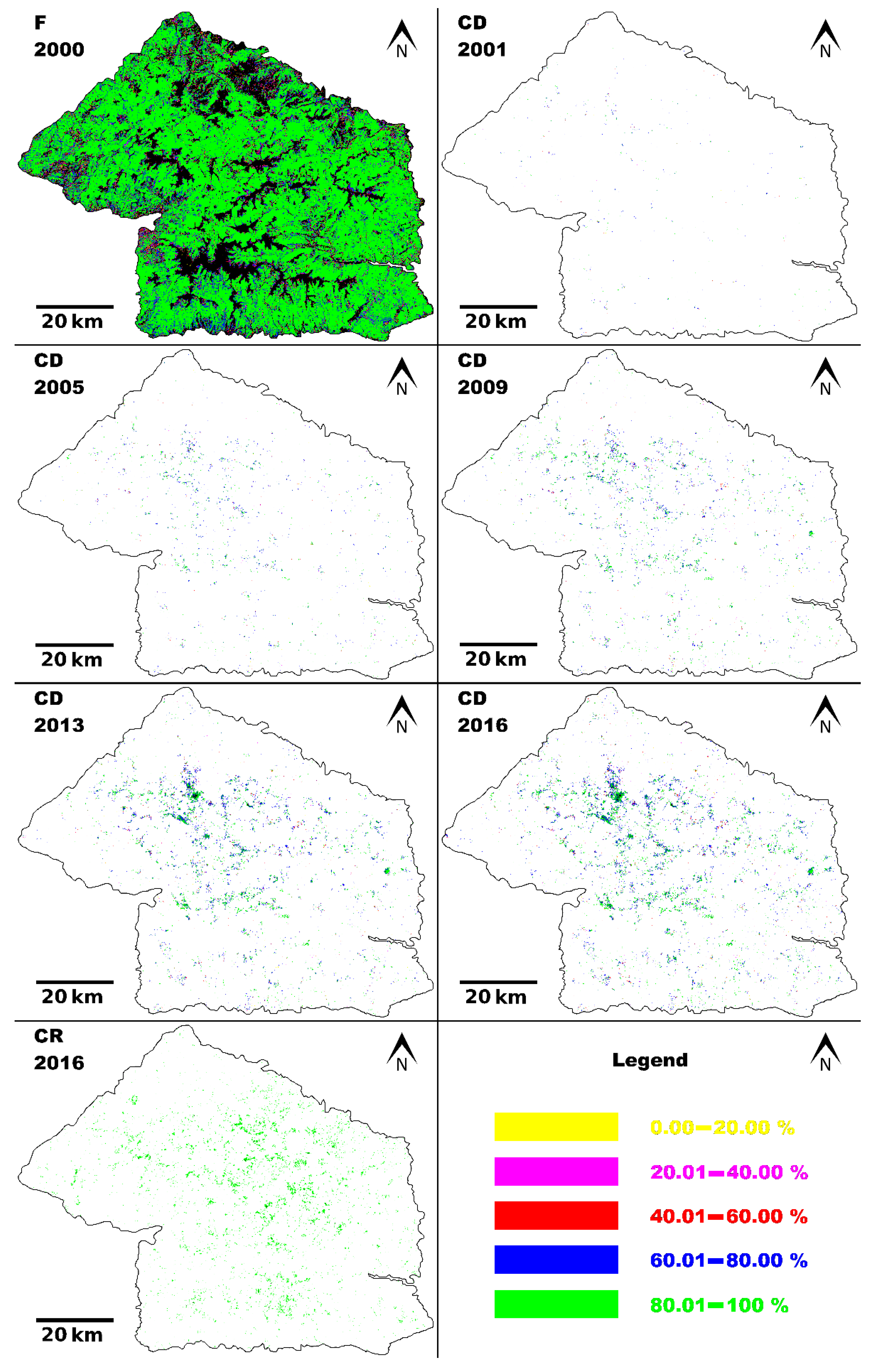
| 0–20% | 20.1–40% | 40.1–60% | 60.1–80% | 80.1–100% | |
|---|---|---|---|---|---|
| TC 2000 | 1.7 | 2.1 | 3.9 | 12.4 | 79.8 |
| L 2001 | 5.3 | 4.2 | 14.5 | 38.0 | 38.1 |
| L 2002 | 3.2 | 2.3 | 8.7 | 40.1 | 45.8 |
| L 2003 | 2.6 | 2.3 | 5.9 | 40.4 | 48.8 |
| L 2004 | 3.6 | 3.5 | 9.1 | 36.0 | 47.8 |
| L 2005 | 3.4 | 2.5 | 8.5 | 37.5 | 48.0 |
| L 2006 | 2.9 | 2.7 | 7.8 | 36.0 | 50.7 |
| L 2007 | 3.5 | 2.7 | 8.6 | 36.8 | 48.5 |
| L 2008 | 2.6 | 2.1 | 8.1 | 37.0 | 50.2 |
| L 2009 | 2.5 | 2.2 | 7.7 | 37.1 | 50.6 |
| L 2010 | 2.7 | 2.2 | 7.8 | 36.2 | 51.1 |
| L 2011 | 2.2 | 2.1 | 7.0 | 37.1 | 51.6 |
| L 2012 | 2.7 | 2.3 | 7.2 | 38.6 | 49.4 |
| L 2013 | 3.3 | 2.8 | 9.5 | 39.6 | 44.8 |
| L 2014 | 2.7 | 2.0 | 7.9 | 36.6 | 50.8 |
| L 2015 | 0.2 | 0.2 | 0.8 | 4.1 | 94.8 |
| L 2016 | 1.1 | 1.1 | 5.9 | 41.1 | 50.8 |
| L 2001–2016 | 2.1 | 1.7 | 6.5 | 41.7 | 48.0 |
| G 2001–2014 | 1.4 | 1.1 | 2.6 | 4.1 | 90.8 |
| TC 2016 | 5.2 | 2.4 | 4.0 | 12.1 | 76.3 |
| H1D and H2D | H1D and Areas (ha) | H2D and Areas (ha) | |
|---|---|---|---|
| Cumulative loss areas | 0.779 | 0.898 | 0.596 |
| Loss areas | 0.359 | 0.799 | 0.129 |
| Tree cover areas | 0.997 | 0.991 | 0.997 |
| H1D and H2D | H1D and Areas (ha) | H2D and Areas (ha) | |
|---|---|---|---|
| Cumulative loss areas | 49.5 (n = 15, <0.001) | 123.1 (n = 15, <0.001) | 20.7 (n = 16, <0.001) |
| Loss areas | 7.8 (n = 15, 0.014) | 55.5 (n = 15, <0.001) | 2.1 (n = 16, 0.172) |
| Tree cover areas | 5257.5 (n = 15, <0.001) | 1669.6 (n = 15, <0.001) | 4506 (n = 16, <0.001) |
| H1D and H2D | H1D and Areas (ha) | H2D and Areas (ha) | |
|---|---|---|---|
| Cumulative loss areas | <0.001 | <0.001 | <0.001 |
| Loss areas | 0.014 | <0.001 | 0.172 |
| Tree cover areas | <0.001 | <0.001 | <0.001 |
| H1D and H2D | H1D and Areas (ha) | H2D and Areas (ha) | |
|---|---|---|---|
| Cumulative loss areas | 0.756 | −0.985 | −0.759 |
| Loss areas | 0.321 | −0.565 | −0.088 |
| Tree cover areas | 1.00 | −1.00 | −1.00 |
Publisher’s Note: MDPI stays neutral with regard to jurisdictional claims in published maps and institutional affiliations. |
© 2021 by the authors. Licensee MDPI, Basel, Switzerland. This article is an open access article distributed under the terms and conditions of the Creative Commons Attribution (CC BY) license (https://creativecommons.org/licenses/by/4.0/).
Share and Cite
Simion, A.G.; Andronache, I.; Ahammer, H.; Marin, M.; Loghin, V.; Nedelcu, I.D.; Popa, C.M.; Peptenatu, D.; Jelinek, H.F. Particularities of Forest Dynamics Using Higuchi Dimension. Parâng Mountains as a Case Study. Fractal Fract. 2021, 5, 96. https://doi.org/10.3390/fractalfract5030096
Simion AG, Andronache I, Ahammer H, Marin M, Loghin V, Nedelcu ID, Popa CM, Peptenatu D, Jelinek HF. Particularities of Forest Dynamics Using Higuchi Dimension. Parâng Mountains as a Case Study. Fractal and Fractional. 2021; 5(3):96. https://doi.org/10.3390/fractalfract5030096
Chicago/Turabian StyleSimion, Adrian Gabriel, Ion Andronache, Helmut Ahammer, Marian Marin, Vlad Loghin, Iulia Daniela Nedelcu, Cristian Mihnea Popa, Daniel Peptenatu, and Herbert Franz Jelinek. 2021. "Particularities of Forest Dynamics Using Higuchi Dimension. Parâng Mountains as a Case Study" Fractal and Fractional 5, no. 3: 96. https://doi.org/10.3390/fractalfract5030096
APA StyleSimion, A. G., Andronache, I., Ahammer, H., Marin, M., Loghin, V., Nedelcu, I. D., Popa, C. M., Peptenatu, D., & Jelinek, H. F. (2021). Particularities of Forest Dynamics Using Higuchi Dimension. Parâng Mountains as a Case Study. Fractal and Fractional, 5(3), 96. https://doi.org/10.3390/fractalfract5030096