A Modified Leslie–Gower Model Incorporating Beddington–DeAngelis Functional Response, Double Allee Effect and Memory Effect

Abstract

In this paper, a modified Leslie–Gower predator-prey model with Beddington–DeAngelis functional response and double Allee effect in the growth rate of a predator population is proposed. In order to consider memory effect on the proposed model, we employ the Caputo fractional-order derivative. We investigate the dynamic behaviors of the proposed model for both strong and weak Allee effect cases. The existence, uniqueness, non-negativity, and boundedness of the solution are discussed. Then, we determine the existing condition and local stability analysis of all possible equilibrium points. Necessary conditions for the existence of the Hopf bifurcation driven by the order of the fractional derivative are also determined analytically. Furthermore, by choosing a suitable Lyapunov function, we derive the sufficient conditions to ensure the global asymptotic stability for the predator extinction point for the strong Allee effect case as well as for the prey extinction point and the interior point for the weak Allee effect case. Finally, numerical simulations are shown to confirm the theoretical results and can explore more dynamical behaviors of the system, such as the bi-stability and forward bifurcation.

1. Introduction

Modeling interaction between prey and its predator has become a dominant topic in mathematical biology due to its ubiquitous existence and fundamentality in many biological systems. Study of the dynamics of the predator-prey model could provide qualitative explanations of numerous phenomena that can occur in predator and prey interaction. One of the crucial phenomenon in ecology that influences the per capita growth rate either in the predator or prey population is the Allee effect, which describes a condition where, at low population densities, the per capita growth rate of the population has a positive dependence with its density. There are two kinds of Allee effects, namely the strong Allee effect and the weak Allee effect. In the strong Allee effect, there is a population threshold value named the Allee threshold, below which the per capita growth rate of the population is negative [1,2]. In terms of conservation biology, if the Allee threshold is larger, then it places a population at higher risk of extinction in a low-density population. Meanwhile, in the weak Allee effect, the per capita growth rate of the population always remains positive but is still reduced at low population densities [3,4,5]. If two or more mechanisms that generate the Allee effect works simultaneously on a single population, then it is known as the double (or multiple) Allee effect [6,7]. Biological evidence of such phenomenon from both terrestrial and aquatic habitat is given in Table 2 of [7,8] and the references cited therein.

From the mathematical point of view, some scholars have been investigating the dynamics of predator-prey models with the Allee effect in the prey population [9,10,11,12,13] or predator population [14,15,16]. The main focus of all the mentioned research studies is to investigate whether the Allee effect has a tremendous impact on the occurrence of various dynamics in the predator-prey model. For the double Allee effect phenomenon, there are some papers that study the double Allee effect in the prey, see for example [17,18]. However, most of the studies just focused on the double Allee effect in the growth of prey population, although observations are showing that the double Allee effect could be discovered in the growth of the predator population. A typical example comes from the endangered species African wild dog (Lycaon pictus). Their social system requires a high population density to survive and reproduce. Being a predator, the African wild dog is a generalist species with the Thomson’s gazelle (Eudorcas thomsonii) as their common prey but it also hunts other animals such as the impala (Aepyceros melampus), warthog (Phacochoerus aethiopicus), hares, etc. They live in permanent packs of about 27 adults and pups and have to share food after killing their prey. There is also interference among predators in their hunting behavior. We refer the readers to [19] for details.

In the natural world, the presence of memory must exist in prey and predator interaction since the growth rates of prey and predator at any point depend on the history of the variables at all previous times and not only on the current state which is local to that point [20,21,22,23,24]. Recently, fractional calculus through the fractional derivatives has been known to provide an excellent instrument for describing the memory and hereditary properties of various materials and processes [25], such as in biology, finance, engineering, and physics (see, for example, [26,27,28,29,30] and the references therein). Some interesting papers regarding the Allee effect in the fractional-order predator-prey models are provided in [31,32]. In [31], Suryanto et al. have studied the local stability of the modified Leslie–Gower model with the Beddington–DeAngelis functional response and additive Allee effect in the prey population. They construct the numerical scheme that preserves the dynamics of its first-order system provided by [33]. Later, in [32], Baisad and Moonchai considered the Gause predator-prey model that includes the Allee effect in the prey population and Holling type-III functional response. They also studied the local stability and sufficient conditions of a Hopf bifurcation at the positive equilibrium point. In both papers, the dynamical behaviors are influenced by the order of the derivative.

Motivated by the above mentioned points, this paper aims to study the fractional-order Leslie–Gower predator-prey model incorporating the Beddington–DeAngelis functional response and double Allee effect. The proposed model includes the Caputo fractional-order derivative to capture the effect of memory in the growth rates of both prey and predator. From what we know, the dynamic of our proposed model that incorporates the double Allee effect in the growth of predator and memory effect under the Caputo fractional-order derivative has not been proposed and investigated by other scholars. This work may reveal an interesting ecological point of view to the importance of the double Allee effect than the single Allee effect towards the management of exploited or threatened predator population.

The remaining part of this paper is organized as follows. In Section 2, the model formulation is given. The existence, uniqueness, non-negativity, and boundedness of solutions of our model are discussed in Section 3. Then, we investigate the dynamic behaviors of the model for both weak and strong Allee effects. In Section 4, the existence of non-negative equilibrium points and the local stability of non-negative equilibrium points along with Hopf bifurcation analysis are presented. Next, the sufficient conditions for the global stability of the equilibrium points are carried out in Section 5. Numerical simulations are shown in Section 6 to verify our analytical findings as well as to numerically explore the impact of capturing rate, the Allee threshold, and the order of the fractional-order system on the dynamics of our model. Finally, we draw conclusions in Section 7.

2. Model Formulation

One of the primary directions in modelling the interaction of prey-predator populations is based on the mass conservation principle, which says that the predators can grow only as a function of what they have consumed. Under this principle, the general model of the predator-prey dynamics takes the following model [34]:

$$\begin{array}{cc}\hfill \frac{dx}{dt}=& f\left(x\right)x-g(x,y)y,\hfill \\ \hfill \frac{dy}{dt}=& kg(x,y)y-\mu y,\hfill \end{array}$$

(1)

where $x\left(t\right)$ and $y\left(t\right)$ are, respectively, the prey and predator population densities at time t, $f\left(x\right)$ is the per capita growth rate of prey, $g(x,y)$ is the functional response, k is the predation efficiency, and $\mu$ is the predator per capita death rate. An alternative to the conservative predator-prey model (1) is to abandon the mass conservation principle. This type of model does not explicitly describe the relationship between predation rate and the reproduction rate of predator. A foremost predator-prey model in this direction is the Leslie–Gower model [35]. The Leslie–Gower model maintains the prey equation as in system (1) but applies a logistic type of model for the predator equation. By considering that the per capita growth rate of prey obeys the logistic growth and that predation follows the Beddington–DeAngelis functional response, we have the following Leslie–Gower model.

$$\begin{array}{cc}\hfill \frac{dx}{dt}=& \widehat{r}x-{\widehat{\beta }}_1{x}^2-\frac{\widehat{b}xy}{1+\widehat{c}x+\widehat{q}y},\hfill \\ \hfill \frac{dy}{dt}=& \widehat{s}y-\widehat{\sigma }{y}^2.\hfill \end{array}$$

(2)

Notice that the logistic type forms in both prey and predator equations are written in the form as suggested by [36]. This typical logistic form is for avoiding paradoxes in the logistic equation [37,38]. All parameters $\widehat{r},{\widehat{\beta }}_1,\widehat{b},\widehat{c},\widehat{q},\widehat{s},\widehat{\sigma }$ in the system (2) are real and positive. The ecological meaning of the parameters are as follows: $\widehat{r}$ and ${\widehat{\beta }}_1$ are the intrinsic growth rate of the prey and the prey intraspecific competition coefficient in the absence of predation, respectively; $\widehat{s}$ and $\widehat{\sigma }$ are the intrinsic growth rate of the predator and the predator intraspecific competition coefficient, respectively; $\widehat{b}$ and $\widehat{c}$ measure the effect of capturing rate and handling time by the predator to the predation rate, respectively; $\widehat{q}$ is the strength of interference among predators. The coefficient of predator intraspecific competition is assumed to depend on the prey density, i.e., $\widehat{\sigma }=\frac{{\widehat{\beta }}_2}{x}$, where ${\widehat{\beta }}_2$ is the constant of predator intraspecific competition. Such assumption makes sense because when the prey is available in abundant $(x\to \infty )$, then there will no intraspecific competition $(\widehat{\sigma }\to 0)$ and the predator can attain its maximum per capita growth rate $\widehat{s}$. On the contrary, if the prey is rare $(x\to 0)$, then the intraspecific competition becomes maximum $(\widehat{\sigma }\to \infty )$ and, hence, the predator will become extinct as the per capita growth rate of predator becomes $-\infty$. When a severe scarcity of prey occurs, the predator can switch to alternative populations, which causes the reduction in intraspecific competition for hunting the favourite food x. To account for such phenomenon, Aziz-Alaoui and Okiye [39] proposed a modified Leslie–Gower model by introducing an inhibition coefficient $(\widehat{l})$ in the intraspecific competition due to the availability of alternative food for the predator. The intraspecific competition coefficient now becomes $\widehat{\sigma }=\frac{{\widehat{\beta }}_2}{\widehat{l}+x}$. The modified Leslie–Gower model with the Beddington–DeAngelis functional response has been studied in [40,41]. Today, the Leslie–Gower type model still attracts many scholars (see [42,43,44] and the references therein).

In this paper, we reconsider the modified Leslie–Gower predator-prey model (2) but we assume that the intrinsic growth rate of the predator population is affected by the double Allee effect. Then the predator-prey model (2) takes the following form:

$$\begin{array}{cc}\hfill \frac{dx}{dt}=& \widehat{r}x-{\widehat{\beta }}_1{x}^2-\frac{\widehat{b}xy}{1+\widehat{c}x+\widehat{q}y},\hfill \\ \hfill \frac{dy}{dt}=& \widehat{s}\left(\frac{y-\widehat{m}}{y+\widehat{n}}\right)y-\frac{{\widehat{\beta }}_2}{\widehat{l}+x}{y}^2,\hfill \end{array}$$

(3)

where $\widehat{m}$ is the Allee threshold, $\widehat{n}$ is the auxiliary Allee effect constant with $\widehat{n}>0$ and $\widehat{n}>-\widehat{m}$. In the second equation of model (3), the intrinsic growth rate of the predator $\widehat{s}$ is affected by double Allee effects. Without the intraspecific competition for the predator, the per capita growth rate of the predator is reduced from $\widehat{s}$ to $\widehat{s}\left(\frac{y-\widehat{m}}{y+\widehat{n}}\right)$ due to the Allee effect [45]. Therefore, the Allee effect is strong if $\widehat{m}>0$ and weak if $-\widehat{n}<\widehat{m}\le 0$ [9,18].

In order to seize the entire time population growth condition, we consider a fractional-order derivative to the left-hand side of the classical derivative system (3) as follows:

$$\begin{array}{cc}\hfill D_{*}^{\alpha }x=& \widehat{r}x-{\widehat{\beta }}_1{x}^2-\frac{\widehat{b}xy}{1+\widehat{c}x+\widehat{q}y},\hfill \\ \hfill D_{*}^{\alpha }y=& \widehat{s}\left(\frac{y-\widehat{m}}{y+\widehat{n}}\right)y-\frac{{\widehat{\beta }}_2}{\widehat{l}+x}{y}^2,\hfill \end{array}$$

(4)

with initial conditions $x\left(0\right)>0$ and $y\left(0\right)>0$. $D_{*}^{\alpha }$ represents the Caputo fractional-order derivative of a real valued function f, which is defined by the following:

$$D_{*}^{\alpha }f\left(t\right)=\frac{1}{\mathrm{\Gamma }(n-\alpha )}{\int }_0^t\frac{f^n\left(\tau \right)}{{(t-\tau )}^{n-\alpha -1}}d\tau ,$$

where $\mathrm{\Gamma }(·)$ is the Gamma function and $\alpha \in (n-1,n],n\in {\mathbb{Z}}^{+}$ [25].

In order to overcome the inconsistency of time dimension between the left-hand side of system (4) with its right-hand side, we follow [46,47,48] to modify all of the biological parameters in the right-hand side that have time dimension ($tim{e}^{-1}$). Thus, we have a new system.

$$\begin{array}{cc}\hfill D_{*}^{\alpha }x=& {\widehat{r}}^{\alpha }x-{\widehat{\beta }}_1^{\alpha }{x}^2-\frac{{\widehat{b}}^{\alpha }xy}{1+\widehat{c}x+\widehat{q}y},\hfill \\ \hfill D_{*}^{\alpha }y=& {\widehat{s}}^{\alpha }\left(\frac{y-\widehat{m}}{y+\widehat{n}}\right)y-\frac{{\widehat{\beta }}_2^{\alpha }}{\widehat{l}+x}{y}^2.\hfill \end{array}$$

(5)

For simplification, we replace system (5) with the redefined parameters as follows:

$$\begin{array}{cc}\hfill D_{*}^{\alpha }x=& rx-{\beta }_1{x}^2-\frac{bxy}{1+cx+qy},\hfill \\ \hfill D_{*}^{\alpha }y=& s\left(\frac{y-m}{y+n}\right)y-\frac{{\beta }_2}{l+x}{y}^2,\hfill \end{array}$$

(6)

where

$${\widehat{r}}^{\alpha }=r,{\widehat{\beta }}_1^{\alpha }={\beta }_1,{\widehat{b}}^{\alpha }=b,\widehat{c}=c,\widehat{q}=q,{\widehat{s}}^{\alpha }=s,\widehat{m}=m,\widehat{n}=n,{\widehat{\beta }}_2^{\alpha }={\beta }_2,\widehat{l}=l.$$

Notice that, the authors [49] have studied the local stability and have shown numerically a Hopf bifurcation circumstance around the interior point for the case of $m=0$. In this paper, we focus on the local and global dynamics of system (6) for both $m>0$ and $m<0$ cases.

3. Preliminaries Results

In this section, we bring out the fact that system (6) is biologically well-behaved by showing that the solution of system (6) exists and is unique as well being non-negative and bounded.

3.1. Existence and Uniqueness

The existence and uniqueness of the solution of system (6) are examined in the region $\mathrm{\Omega }\times [0,T],$ where $\mathrm{\Omega }=\{(x,y)\in {\mathbb{R}}^2:\max \left\{\right|x|,|y\left|\right\}\le M\}$ and $T<+\infty$. Let a mapping $F\left(Z\right)=(F_1\left(Z\right),F_2\left(Z\right))$ with the following.

$$\begin{array}{cc}\hfill F_1\left(Z\right)=& rx-{\beta }_1{x}^2-\frac{bxy}{1+cx+qy},\hfill \\ \hfill F_2\left(Z\right)=& \frac{s{y}^2}{y+n}-\frac{msy}{y+n}-\frac{{\beta }_2{y}^2}{l+x}.\hfill \end{array}$$

(7)

For any $Z=(x,y),\overline{Z}=(\overline{x},\overline{y}),Z,\overline{Z}\in \mathrm{\Omega }$, it follows from (7) that the following is the case:

$$\begin{array}{ccc}\hfill \left|\right|F\left(Z\right)-F\left(\overline{Z}\right)\left|\right|& \hfill =& |F_1\left(Z\right)-F_1\left(\overline{Z}\right)|+|F_2\left(Z\right)-F_2\left(\overline{Z}\right)|\hfill \\ & \hfill =& \left|r(x-\overline{x})-{\beta }_1(x^2-{\overline{x}}^2)-b\left(\frac{xy}{1+cx+qy}-\frac{\overline{x}\overline{y}}{1+c\overline{x}+q\overline{y}}\right)\right|+\hfill \\ & & \left|s\left(\frac{y^2}{y+n}-\frac{{\overline{y}}^2}{\overline{y}+n}\right)-ms\left(\frac{y}{y+n}-\frac{\overline{y}}{\overline{y}+n}\right)-{\beta }_2\left(\frac{y^2}{l+x}-\frac{{\overline{y}}^2}{l+\overline{x}}\right)\right|\hfill \\ & \hfill \le & r|x-\overline{x}|+{\beta }_1|x^2-{\overline{x}}^2|+b\left|\frac{xy(1+c\overline{x}+q\overline{y})-\overline{x}\overline{y}(1+cx+qy)}{(1+cx+qy)(1+c\overline{x}+q\overline{y})}\right|\hfill \\ & & +s\left|\frac{y^2(\overline{y}+n)-{\overline{y}}^2(y+n)}{(y+n)(\overline{y}+n)}\right|+\left|m\right|s\left|\frac{y(\overline{y}+n)-\overline{y}(y+n)}{(y+n)(\overline{y}+n)}\right|\hfill \\ & & +{\beta }_2\left|\frac{y^2(l+\overline{x})-{\overline{y}}^2(l+x)}{(l+x)(l+\overline{x})}\right|\hfill \\ & \hfill =& r|x-\overline{x}|+{\beta }_1|x+\overline{x}\left|\right|x-\overline{x}|\hfill \\ & & +b\left|\frac{(x+cx\overline{x})(y-\overline{y})+(\overline{y}+qy\overline{y})(x-\overline{x})}{(1+cx+qy)(1+c\overline{x}+q\overline{y})}\right|\hfill \\ & & +s\left|\frac{(y\overline{y}+n(y+\overline{y}))(y-\overline{y})}{(y+n)(\overline{y}+n)}\right|+\left|m\right|s\left|\frac{n(y-\overline{y})}{(y+n)(\overline{y}+n)}\right|\hfill \\ & & +{\beta }_2\left|\frac{(l+x)(y+\overline{y})(y-\overline{y})-y^2(x-\overline{x})}{(l+x)(l+\overline{x})}\right|\hfill \\ & \hfill \le & r|x-\overline{x}|+{\beta }_1|x+\overline{x}\left|\right|x-\overline{x}|+b|(x+cx\overline{x})(y-\overline{y})|\hfill \\ & & +b|(\overline{y}+qy\overline{y})(x-\overline{x})|+\frac{s}{n^2}\left|(y\overline{y}+n(y+\overline{y}))(y-\overline{y})\right|\hfill \\ & & +\frac{\left|m\right|s}{n}|y-\overline{y}|+\frac{{\beta }_2}{l^2}|(l+x)(y+\overline{y})(y-\overline{y})-y^2(x-\overline{x})|\hfill \\ & \hfill \le & r|x-\overline{x}|+2{\beta }_{1}M|x-\overline{x}|+(bM+bc{M}^2)|y-\overline{y}|\hfill \\ & & +(bM+bq{M}^2)|x-\overline{x}|+\left(\frac{s{M}^2}{n^2}+\frac{2sM}{n}\right)|y-\overline{y}|+\frac{\left|m\right|s}{n}|y-\overline{y}|\hfill \\ & & +\left(\frac{2{\beta }_{2}M}{l}+\frac{2{\beta }_2{M}^2}{l^2}\right)|y-\overline{y}|+\frac{{\beta }_2{M}^2}{l^2}|x-\overline{x}|\hfill \\ & \hfill =& L_1|x-\overline{x}|+L_2|y-\overline{y}|\hfill \\ & \hfill \le & L\left|\right|Z-\overline{Z}\left|\right|\hfill \end{array}$$

where

$$\begin{array}{cc}\hfill L_1=& r+(2{\beta }_1+b)M+\left(bq+\frac{{\beta }_2}{l^2}\right)M^2,\hfill \\ \hfill L_2=& \frac{\left|m\right|s}{n}+\left(b+\frac{2s}{n}+\frac{2{\beta }_2}{l}\right)M+\left(bc+\frac{s}{n^2}+\frac{2{\beta }_2}{l^2}\right)M^2,\hfill \\ \hfill L=& \max \left\{L_1,L_2\right\}.\hfill \end{array}$$

Since $F\left(Z\right)$ satisfies the Lipschitz condition with respect to Z, it follows from Theorem 3.7 in [50] that there exists a unique solution $Z\left(t\right)$ of system (6) with initial condition $Z\left(0\right)=\left(x\right(0),y(0\left)\right)$. Consequently, we have the following theorem.

Theorem 1.

For each $Z\left(0\right)=\left(x\right(0),y(0\left)\right)\in \mathrm{\Omega }$, then initial value problem of system (6) has a unique solution $Z\left(t\right)\in \mathrm{\Omega }$ which is defined for all $t\ge 0$.

3.2. Non-Negativity and Boundedness

In order to prove that all solutions of system (6) are non-negative and bounded, let ${\mathbb{R}}_{+}^2=\{W={(x,y)}^T\in {\mathbb{R}}^2|x\left(t\right)\ge 0,y\left(t\right)\ge 0\}$ be the non-negative quadrant on the $xy-$plane. In the case of the biological significance, we must ensure that when the initial condition starts in ${\mathbb{R}}_{+}^2$, then the solution of system (6) remains in ${\mathbb{R}}_{+}^2$ for all $t\ge t_0$.

Theorem 2.

If $x\left(t_0\right)\ge 0$ and $y\left(t_0\right)\ge 0$, then all solutions of the system (6) are non-negative and uniformly bounded.

Proof. 

Let $W\left(t_0\right)=\left(\begin{array}{c}x\left(t_0\right)\\ y\left(t_0\right)\end{array}\right)\in {\mathbb{R}}_{+}^2$ and assume that $W\left(t\right)=\left(\begin{array}{c}x\left(t\right)\\ y\left(t\right)\end{array}\right)$ for $t\ge t_0$ be the solutions of system (6).

Suppose that assumption is false, then there exists $t^{*}>t_0$ such that $W\left(t\right)>0$ for $t_0\le t<t^{*}$, $W\left(t^{*}\right)=0$, and $W\left(t_{+}^{*}\right)<0$ for $t_{+}^{*}>t^{*}$. From system (6), one has the following.

$$D_{*}^{\alpha }{W\left(t\right)|}_{t=t^{*}}=0.$$

(8)

Based on Lemma 1 in [51], we have $W\left(t_{+}^{*}\right)=0$, which contradicts with $W\left(t_{+}^{*}\right)<0$ for $t_{+}^{*}>t^{*}$. Therefore, we conclude $W\left(t\right)\ge 0$ for all $t\ge 0$.

Next, we prove the boundedness of all solutions of system (6). From the first equation of system (6), we have the following.

$$\begin{array}{cc}\hfill D_{*}^{\alpha }x\left(t\right)+x\left(t\right)=& rx-{\beta }_1{x}^2-\frac{bxy}{1+cx+qy}+x\hfill \\ \hfill =& -{\beta }_1{x}^2+(1+r)x-\frac{bxy}{1+cx+qy}\hfill \\ \hfill =& -{\beta }_1{\left(x-\frac{(1+r)}{2{\beta }_1}\right)}^2+\frac{{(1+r)}^2}{4{\beta }_1}-\frac{bxy}{1+cx+qy}\hfill \\ \hfill \le & \frac{{(1+r)}^2}{4{\beta }_1}.\hfill \end{array}$$

By Lemma 3 in [51], we have the following:

$$x\left(t\right)\le \left(x\left(t_0\right)-\frac{{(1+r)}^2}{4{\beta }_1}\right)E_{\alpha }\left[-{(t-t_0)}^{\alpha }\right]+\frac{{(1+r)}^2}{4{\beta }_1}\to \frac{{(1+r)}^2}{4{\beta }_1},t\to \infty ,$$

(9)

where $E_{\alpha }$ is the Mittag–Leffler function. Therefore, $x\left(t\right)$ with initial condition $x\left(t_0\right)$ are confined to the region ${\mathrm{\Omega }}_1$ where the following is the case.

$${\mathrm{\Omega }}_1=\left\{x\left(t\right)\le \frac{{(1+r)}^2}{4{\beta }_1}+{ϵ}_1={\gamma }_1,{ϵ}_1>0\right\}.$$

(10)

From the second equation of system (6), we have the following.

$$\begin{array}{cc}\hfill D_{*}^{\alpha }y\left(t\right)+sy\left(t\right)=& \frac{s{y}^2}{y+n}-\frac{msy}{y+n}-\frac{{\beta }_2{y}^2}{l+x}+sy.\hfill \end{array}$$

We also have $x\left(t\right)\le {\gamma }_1$ from (10), then the following obtains.

$$\begin{array}{cc}\hfill D_{*}^{\alpha }y\left(t\right)+sy\left(t\right)\le & \frac{s{y}^2}{y+n}-\frac{msy}{y+n}-\frac{{\beta }_2{y}^2}{l+{\gamma }_1}+sy\hfill \\ \hfill \le & \frac{s{y}^2}{y}-\frac{msy}{y+n}-\frac{{\beta }_2{y}^2}{l+{\gamma }_1}+sy\hfill \\ \hfill =& -\frac{{\beta }_2{y}^2}{l+{\gamma }_1}+2sy-\frac{msy}{y+n}\hfill \\ \hfill =& -\frac{{\beta }_2}{l+{\gamma }_1}{\left(y-\frac{(l+{\gamma }_1)s}{{\beta }_2}\right)}^2+\frac{(l+{\gamma }_1)s^2}{{\beta }_2}-\frac{msy}{y+n}\hfill \\ \hfill \le & \frac{(l+{\gamma }_1)s^2}{{\beta }_2}\hfill \end{array}$$

Again by using Lemma 3 in [51], for the strong Allee effect $(m>0)$, we have the following.

$$y\left(t\right)\le \left(y\left(t_0\right)-\frac{(l+{\gamma }_1)s}{{\beta }_2}\right)E_{\alpha }\left[-s{(t-t_0)}^{\alpha }\right]+\frac{(l+{\gamma }_1)s}{{\beta }_2}\to \frac{(l+{\gamma }_1)s}{{\beta }_2},t\to \infty .$$

(11)

However, for the weak Allee effect $(m<0)$, we have the following.

$$\begin{array}{c}y\left(t\right)\le \left(y\left(t_0\right)-\left(\frac{(l+{\gamma }_1)s}{{\beta }_2}-m\right)\right)E_{\alpha }\left[-s{(t-t_0)}^{\alpha }\right]\hfill \\ \hfill +\left(\frac{(l+{\gamma }_1)s}{{\beta }_2}-m\right)\to \left(\frac{(l+{\gamma }_1)s}{{\beta }_2}-m\right),t\to \infty .\end{array}$$

(12)

Therefore, the solution of $y\left(t\right)$ with initial condition $y\left(t_0\right)$ are confined to region ${\mathrm{\Omega }}_2$ where

$${\mathrm{\Omega }}_2=\left\{y\left(t\right)\le {\gamma }_2\right\},$$

(13)

and where the following is the case.

$${\gamma }_2=\left\{\begin{array}{ccc}\frac{(l+{\gamma }_1)s}{{\beta }_2}+{ϵ}_2,\hfill & {ϵ}_2>0,\hfill & m>0\hfill \\ \left(\frac{(l+{\gamma }_1)s}{{\beta }_2}-m\right)+{ϵ}_2,\hfill & {ϵ}_2>0,\hfill & m<0\hfill \end{array}\right.$$

□

4. Equilibrium Points and Their Local Stability

In this section, the equilibrium points and existence conditions are obtained and their local stability is analyzed by using the Matignon condition [25] for the weak $(m<0)$ and the strong $(m>0)$ Allee effect, respectively.

(1)

The equilibrium points of system (6) for the weak Allee effect $(m<0)$ are as follows:

(a)

Both prey and predator extinction point $W_0=(0,0)$, which always exists;

(b)

The predator extinction point $W_1=(\frac{r}{{\beta }_1},0)$, which always exists;

(c)

The prey extinction point $W_2=\left(0,{\overline{y}}_w\right)$ where we have the following.

$${\overline{y}}_w={\displaystyle \frac{\frac{ls}{{\beta }_2}-n}{2}}+{\displaystyle \frac{\sqrt{{(\frac{ls}{{\beta }_2}-n)}^2-4\frac{mls}{{\beta }_2}}}{2}}$$

Denote $W_2$ as always existing.

(d)

The interior point $\widehat{W}=({\widehat{x}}_w,{\widehat{y}}_w)$ where ${\widehat{x}}_w={\displaystyle \frac{{\beta }_2{\widehat{y}}_w({\widehat{y}}_w+n)}{s({\widehat{y}}_w-m)}}-l$ and ${\widehat{y}}_w$ are all positive roots of the quartic equation (14):

$$a_1{y}^4+a_2{y}^3+a_3{y}^2+a_{4}y+a_5=0,$$

(14)

where

$$\begin{array}{cc}\hfill a_1=& {\beta }_1{\beta }_{2}qs+c{\beta }_1{\beta }_2^2,\hfill \\ \hfill a_2=& (b-qr-lq{\beta }_1)s^2+({\beta }_1{\beta }_2(1+nq-mq-2cl)-cr{\beta }_2)s+2c{\beta }_1{\beta }_2^{2}n,\hfill \\ \hfill a_3=& (c{\beta }_1{l}^2+2lmq{\beta }_1+lcr+2mqr-2bm-l{\beta }_1-r)s^2\hfill \\ & +({\beta }_1{\beta }_2(2clm-2cln-nmq-m+n)+cr{\beta }_2(m-n))s+c{\beta }_1{\beta }_2^2{n}^2,\hfill \\ \hfill a_4=& (-2c{l}^{2}m{\beta }_1-l{m}^{2}q{\beta }_1-2clmr-m^{2}qr+b{m}^2+2lm{\beta }_1+2mr)s^2\hfill \\ & +(2clmn{\beta }_1{\beta }_2+cmnr{\beta }_2-mn{\beta }_1{\beta }_2)s,\hfill \\ \hfill a_5=& m^2(cl-1)(l{\beta }_1+r)s^2.\hfill \end{array}$$

(2)

The equilibrium points of system (6) for the strong Allee effect $(m>0)$ are as follows:

(a)

Both prey and predator extinction point $S_0=(0,0)$, which always exists;

(b)

The predator extinction point $S_1=(\frac{r}{{\beta }_1},0)$, which always exists;

(c)

The prey extinction point $S_{2,3}=\left(0,{\overline{y}}_s\right)$ where ${\overline{y}}_s$ is the positive solution of the quadratic equation $y^2-\left(\frac{ls}{{\beta }_2}-n\right)y+\frac{mls}{{\beta }_2}=0$. The existence of $S_{2,3}$ is described as follows:

(i)

If ${\left({\displaystyle \frac{ls}{{\beta }_2}}-n\right)}^2<4{\displaystyle \frac{mls}{{\beta }_2}}$, then the prey extinction point does not exist.

(ii)

If ${\left({\displaystyle \frac{ls}{{\beta }_2}}-n\right)}^2=4{\displaystyle \frac{mls}{{\beta }_2}}$ and $n<{\displaystyle \frac{ls}{{\beta }_2}}$, then there exists a unique prey extinction point, $S_2=S_3=\left(0,{\displaystyle \frac{1}{2}}\left({\displaystyle \frac{ls}{{\beta }_2}}-n)\right)\right)$.

(iii)

If ${\left({\displaystyle \frac{ls}{{\beta }_2}}-n\right)}^2>4{\displaystyle \frac{mls}{{\beta }_2}}$, then there exist two prey extinction points, i.e., the following is the case.

$$S_{2,3}=\left(0,\frac{\frac{ls}{{\beta }_2}-n}{2}\pm {\displaystyle \frac{\sqrt{{(\frac{ls}{{\beta }_2}-n)}^2-4\frac{mls}{{\beta }_2}}}{2}}\right)$$

(d)

The interior point $\widehat{S}=({\widehat{x}}_s,{\widehat{y}}_s)$ exists if ${\widehat{y}}_s>m$ where ${\widehat{x}}_s={\displaystyle \frac{{\beta }_2{\widehat{y}}_s({\widehat{y}}_s+n)}{s({\widehat{y}}_s-m)}}-l$ and ${\widehat{y}}_s$ are also all positive roots of the quartic Equation (14).

In order to study the local stability of system (6) around an equilibrium point $(x^{*},y^{*})$, we consider the following Jacobian matrix J of system (6), which is given by the following.

$$J(x^{*},y^{*})=\left[\begin{array}{cc}{J}_{1,1}& J_{1,2}\\ J_{2,1}& J_{2,2}\end{array}\right]$$

(15)

$$\begin{array}{cc}\hfill J_{1,1}=& r-2{\beta }_1{x}^{*}-{\displaystyle \frac{b{y}^{*}}{1+c{x}^{*}+q{y}^{*}}}+{\displaystyle \frac{bc{x}^{*}{y}^{*}}{{(1+c{x}^{*}+q{y}^{*})}^2}}\hfill \\ \hfill J_{1,2}=& -{\displaystyle \frac{b{x}^{*}}{1+c{x}^{*}+q{y}^{*}}}+{\displaystyle \frac{bq{x}^{*}{y}^{*}}{{(1+c{x}^{*}+q{y}^{*})}^2}}\hfill \\ \hfill J_{2,1}=& {\displaystyle \frac{{\beta }_2{y}^{*2}}{{(l+x^{*})}^2}}\hfill \\ \hfill J_{2,2}=& {\displaystyle \frac{s(y^{*}-m)}{y^{*}+n}}+s{y}^{*}\left({\displaystyle \frac{1}{y^{*}+n}}-{\displaystyle \frac{y^{*}-m}{{(y^{*}+n)}^2}}\right)-{\displaystyle \frac{2{\beta }_2{y}^{*}}{l+x^{*}}}.\hfill \end{array}$$

Theorem 3.

The stability properties of trivial and axial equilibrium points of system (6) for the weak Allee effect $(m<0)$ are as follows:

(a) 

$W_0=(0,0)$ is always unstable.

(b) 

$W_1=(\frac{r}{{\beta }_1},0)$ is always a saddle point.

(c) 

$W_2=(0,{\overline{y}}_w)$ is locally asymptotically stable if $r<{\displaystyle \frac{b{\overline{y}}_w}{1+q{\overline{y}}_w}}$ and $m+n<{\displaystyle \frac{{\beta }_2}{ls}}{({\overline{y}}_w+n)}^2$.

Proof. 

(a)

By substituting $W_0$ to (15), we obtain the Jacobian matrix.

$$J\left(W_0\right)=\left[\begin{array}{cc}r& 0\\ 0& -{\displaystyle \frac{ms}{n}}\end{array}\right].$$

(16)

Therefore, the eigenvalues of (16) are ${\lambda }_1=r>0$ and ${\lambda }_2=-{\displaystyle \frac{ms}{n}}>0$, since $|\arg \left({\lambda }_1\right)|=|\arg \left({\lambda }_2\right)|=0<\frac{\alpha \pi }{2}$, $E_0$ is always unstable by the Matignon condition [25].

(b)

By substituting $W_1$ to (15), we obtain the Jacobian matrix.

$$J\left(W_1\right)=\left[\begin{array}{cc}-r& -{\displaystyle \frac{br}{cr+{\beta }_1}}\\ 0& -{\displaystyle \frac{ms}{n}}\end{array}\right].$$

(17)

The Jacobian matrix (17) has eigenvalues ${\lambda }_1=-r<0$ and ${\lambda }_2=-{\displaystyle \frac{ms}{n}}>0$, showing that $|\arg \left({\lambda }_1\right)|=\pi >\frac{\alpha \pi }{2}$ and $|\arg \left({\lambda }_2\right)|=0<\frac{\alpha \pi }{2}$. Hence, $W_1$ is always a saddle point.

(c)

By evaluating (15) at $W_2$, we obtain the following.

$$J\left(W_2\right)=\left[\begin{array}{cc}r-{\displaystyle \frac{b{\overline{y}}_w}{1+q{\overline{y}}_w}}& 0\\ {\displaystyle \frac{{\beta }_2{\overline{y}}_w^2}{l^2}}& \left({\displaystyle \frac{s(m+n)}{{({\overline{y}}_w+n)}^2}}-{\displaystyle \frac{{\beta }_2}{l}}\right){\overline{y}}_w\end{array}\right].$$

(18)

The eigenvalues of (18) are as follows.

$${\lambda }_1=r-{\displaystyle \frac{b{\overline{y}}_w}{1+q{\overline{y}}_w}}\mathrm{and}{\lambda }_2=\left({\displaystyle \frac{s(m+n)}{{({\overline{y}}_w+n)}^2}}-{\displaystyle \frac{{\beta }_2}{l}}\right){\overline{y}}_w.$$

Thus, $|\arg \left({\lambda }_1\right)|=\pi >{\displaystyle \frac{\alpha \pi }{2}}$ and $|\arg \left({\lambda }_2\right)|=\pi >{\displaystyle \frac{\alpha \pi }{2}}$, whenever $r<{\displaystyle \frac{b{\overline{y}}_w}{1+q{\overline{y}}_w}}$ and $m+n<{\displaystyle \frac{{\beta }_2}{ls}}{({\overline{y}}_w+n)}^2$.

□

Theorem 4.

Suppose that $m<0$ (weak Allee effect) and the following is the case.

$$\begin{array}{cc}\hfill {\chi }_{1w}=& -\left({\beta }_1{\widehat{x}}_w+{\displaystyle \frac{{\beta }_2{\widehat{y}}_w}{l+{\widehat{x}}_w}}\right)+\left({\displaystyle \frac{bc{\widehat{x}}_w{\widehat{y}}_w}{{(1+c{\widehat{x}}_w+q{\widehat{y}}_w)}^2}}+{\displaystyle \frac{s(m+n){\widehat{y}}_w}{{({\widehat{y}}_w+n)}^2}}\right)\hfill \\ \hfill {\chi }_{2w}=& {\beta }_1{\widehat{x}}_w{\widehat{y}}_w\left({\displaystyle \frac{{\beta }_2}{l+{\widehat{x}}_w}}-{\displaystyle \frac{s(m+n)}{{({\widehat{y}}_w+n)}^2}}\right)\hfill \\ \hfill & +{\displaystyle \frac{bs{\widehat{x}}_w}{{(1+c{\widehat{x}}_w+q{\widehat{y}}_w)}^2}}\left({\displaystyle \frac{{\beta }_{2}c(m+n){\widehat{y}}_w^2+s(1+c{\widehat{x}}_w){({\widehat{y}}_w-m)}^2}{{\beta }_2{({\widehat{y}}_w+n)}^2}}-{\displaystyle \frac{{\beta }_{2}c{\widehat{y}}_w^2}{s(l+{\widehat{x}}_w)}}\right)\hfill \\ \hfill {\alpha }^{*}=& {\displaystyle \frac{2}{\pi }}\left|{\tan }^{-1}{\displaystyle \frac{\sqrt{4{\chi }_{2w}-{\left({\chi }_{1w}\right)}^2}}{{\chi }_{1w}}}\right|.\hfill \end{array}$$

The interior point $\widehat{W}=({\widehat{x}}_w,{\widehat{y}}_w)$ is locally asymptotically stable if the following is the case:

(i) 

${\chi }_{1w}^2\ge 4{\chi }_{2w}$, ${\chi }_{1w}<0$, and ${\chi }_{2w}>0$.

(ii) 

${\chi }_{1w}^2<4{\chi }_{2w}$, and if ${\chi }_{1w}<0$, or ${\chi }_{1w}>0$ and $\alpha <{\alpha }^{*}$.

Proof. 

By evaluating (15) at the interior equilibrium point $\widehat{W}=({\widehat{x}}_w,{\widehat{y}}_w)$, we obtain the following.

$$J\left(\widehat{W}\right)=\left[\begin{array}{cc}-{\beta }_1{\widehat{x}}_w+{\displaystyle \frac{bc{\widehat{x}}_w{\widehat{y}}_w}{{(1+c{\widehat{x}}_w+q{\widehat{y}}_w)}^2}}& -{\displaystyle \frac{b{\widehat{x}}_w(1+c{\widehat{x}}_w)}{{(1+c{\widehat{x}}_w+q{\widehat{y}}_w)}^2}}\\ {\displaystyle \frac{s^2{({\widehat{y}}_w-m)}^2}{{\beta }_2{({\widehat{y}}_w+n)}^2}}& {\displaystyle \frac{s(m+n){\widehat{y}}_w}{{({\widehat{y}}_w+n)}^2}}-{\displaystyle \frac{{\beta }_2{\widehat{y}}_w}{l+{\widehat{x}}_w}}\end{array}\right]$$

(19)

The Jacobian matrix (19) has polynomial characteristic ${\lambda }^2-{\chi }_{1w}\lambda +{\chi }_{2w}=0$. By utilizing the Routh–Hurwitz criterion for Caputo fractional-order [52], it follows that $\widehat{W}$ is locally asymptotically stable if condition $\left(i\right)$ or $\left(ii\right)$ is satisfied. □

Theorem 5.

The stability properties of trivial and axial equilibrium points of system (6) for strong Allee effect $(m>0)$ are as follows:

(a) 

$S_0=(0,0)$ is a saddle point.

(b) 

$S_1=(\frac{r}{{\beta }_1},0)$ is always locally asymptotically stable.

(c) 

$S_{2,3}=(0,{\overline{y}}_s)$ is locally asymptotically stable if $r<{\displaystyle \frac{b{\overline{y}}_s}{1+q{\overline{y}}_s}}$ and $m+n<{\displaystyle \frac{{\beta }_2}{ls}}{({\overline{y}}_s+n)}^2$.

Proof. 

(a)

By substituting $S_0$ to (15), we obtain the following.

$$J\left(S_0\right)=\left[\begin{array}{cc}r& 0\\ 0& -{\displaystyle \frac{ms}{n}}\end{array}\right].$$

(20)

It is clear that the eigenvalues of (20) are ${\lambda }_1=r>0$ and ${\lambda }_2=-{\displaystyle \frac{ms}{n}}<0$, and $|\arg \left({\lambda }_1\right)|=0<\frac{\alpha \pi }{2}$ and $|\arg \left({\lambda }_2\right)|=\pi >\frac{\alpha \pi }{2}$. Thus, $S_0$ is a saddle point.

(b)

The Jacobian matrix (15) evaluated at $S_1$ is the following:

$$J\left(S_1\right)=\left[\begin{array}{cc}-r& -{\displaystyle \frac{br}{cr+{\beta }_1}}\\ 0& -{\displaystyle \frac{ms}{n}}\end{array}\right],$$

(21)

where its eigenvalues are ${\lambda }_1=-r<0$ and ${\lambda }_2=-{\displaystyle \frac{ms}{n}}<0$, since $|\arg \left({\lambda }_{1,2}\right)|=\pi >\frac{\alpha \pi }{2}$, $S_1$ is always locally asymptotically stable.

(c)

By evaluating (15) at $S_{2,3}$, we acquire the following.

$$J\left(S_{2,3}\right)=\left[\begin{array}{cc}r-{\displaystyle \frac{b{\overline{y}}_s}{1+q{\overline{y}}_s}}& 0\\ {\displaystyle \frac{{\beta }_2{\overline{y}}_s^2}{l^2}}& \left({\displaystyle \frac{s(m+n)}{{({\overline{y}}_s+n)}^2}}-{\displaystyle \frac{{\beta }_2}{l}}\right){\overline{y}}_s\end{array}\right].$$

(22)

The eigenvalues of (22) are as follows.

$${\lambda }_1=r-{\displaystyle \frac{b{\overline{y}}_s}{1+q{\overline{y}}_s}}\mathrm{and}{\lambda }_2=\left({\displaystyle \frac{s(m+n)}{{({\overline{y}}_s+n)}^2}}-{\displaystyle \frac{{\beta }_2}{l}}\right){\overline{y}}_s.$$

(23)

Therefore $S_{2,3}$ is locally asymptotically stable if $r<{\displaystyle \frac{b{\overline{y}}_s}{1+q{\overline{y}}_s}}$ and $m+n<{\displaystyle \frac{{\beta }_2}{ls}}{({\overline{y}}_w+n)}^2$ because in this case $|\arg \left({\lambda }_1\right)|=|\arg \left({\lambda }_2\right)|=\pi >{\displaystyle \frac{\alpha \pi }{2}}$.

□

Theorem 6.

For the case of strong Allee effect $(m>0)$, the interior point $\widehat{S}=({\widehat{x}}_s,{\widehat{y}}_s)$ is locally asymptotically stable if the following is the case:

(i) 

${\chi }_{1s}^2\ge 4{\chi }_{2s}$, ${\chi }_{1s}<0$, and ${\chi }_{2s}>0$.

(ii) 

${\chi }_{1s}^2<4{\chi }_{2s}$, and if ${\chi }_{1s}<0$, or ${\chi }_{1s}>0$ and $\alpha <{\alpha }^{*}$;

where the following is the case.

$$\begin{array}{cc}\hfill {\chi }_{1s}=& -\left({\beta }_1{\widehat{x}}_s+{\displaystyle \frac{{\beta }_2{\widehat{y}}_s}{l+{\widehat{x}}_s}}\right)+\left({\displaystyle \frac{bc{\widehat{x}}_s{\widehat{y}}_s}{{(1+c{\widehat{x}}_s+q{\widehat{y}}_s)}^2}}+{\displaystyle \frac{s(m+n){\widehat{y}}_s}{{({\widehat{y}}_s+n)}^2}}\right)\hfill \\ \hfill {\chi }_{2s}=& {\beta }_1{\widehat{x}}_s{\widehat{y}}_s\left({\displaystyle \frac{{\beta }_2}{l+{\widehat{x}}_s}}-{\displaystyle \frac{s(m+n)}{{({\widehat{y}}_s+n)}^2}}\right)\hfill \\ \hfill & +{\displaystyle \frac{bs{\widehat{x}}_s}{{(1+c{\widehat{x}}_s+q{\widehat{y}}_s)}^2}}\left({\displaystyle \frac{{\beta }_{2}c(m+n){\widehat{y}}_s^2+s(1+c{\widehat{x}}_s){({\widehat{y}}_s-m)}^2}{{\beta }_2{({\widehat{y}}_s+n)}^2}}-{\displaystyle \frac{{\beta }_{2}c{\widehat{y}}_s^2}{s(l+{\widehat{x}}_s)}}\right)\hfill \\ \hfill {\alpha }^{*}=& {\displaystyle \frac{2}{\pi }}\left|{\tan }^{-1}{\displaystyle \frac{\sqrt{4{\chi }_{2s}-{\left({\chi }_{1s}\right)}^2}}{{\chi }_{1s}}}\right|.\hfill \end{array}$$

Proof. 

The Jacobian matrix (15) at interior equilibrium point $\widehat{S}=({\widehat{x}}_s,{\widehat{y}}_s)$ is given by the following.

$$J(\widehat{S})=\left[\begin{array}{cc}-{\beta }_1{\widehat{x}}_s+{\displaystyle \frac{bc{\widehat{x}}_s{\widehat{y}}_s}{{(1+c{\widehat{x}}_s+q{\widehat{y}}_s)}^2}}& -{\displaystyle \frac{b{\widehat{x}}_s(1+c{\widehat{x}}_s)}{{(1+c{\widehat{x}}_s+q{\widehat{y}}_s)}^2}}\\ {\displaystyle \frac{s^2{({\widehat{y}}_s-m)}^2}{{\beta }_2{({\widehat{y}}_s+n)}^2}}& {\displaystyle \frac{s(m+n){\widehat{y}}_s}{{({\widehat{y}}_s+n)}^2}}-{\displaystyle \frac{{\beta }_2{\widehat{y}}_s}{l+{\widehat{x}}_s}}\end{array}\right].$$

(24)

The Jacobian matrix (24) has polynomial characteristic ${\lambda }^2-{\chi }_{1s}\lambda +{\chi }_{2s}=0$. By using the Routh–Hurwitz criterion for Caputo fractional-order [52], the stability condition is completely proven. □

Hopf bifurcation on a fractional-order system occurs when the Jacobian matrix evaluated at an equilibrium point has two complex conjugate eigenvalues and there is a limit-cycle when the stability of that system changes. Here, we use the conditions for the existence of a Hopf bifurcation which was introduced by [53]. According to Theorems 4 and 6, the stability of the interior equilibrium point for both weak and strong Allee effects is influenced by the order of the fractional derivative $\left(\alpha \right)$. Thus, we can establish the condition for the existence of a Hopf bifurcation at the interior point as $\alpha$ passes through the critical value ${\alpha }^{*}$ in the following theorem.

Theorem 7

(Existence of Hopf bifurcation [53]). Let ${\chi }_{1w}^2<4{\chi }_{2w}(or{\chi }_{1s}^2<4{\chi }_{2s})$ and ${\chi }_{1w}>0(or{\chi }_{1s}>0)$. System (6) undergoes a Hopf bifurcation around the interior point $\widehat{W}\left(or\widehat{S}\right)$ when α crosses ${\alpha }^{*}$.

Proof. 

Based on Theorem 6, when ${\chi }_{1s}^2<4{\chi }_{2s}$ and ${\chi }_{1s}>0$, the eigenvalues of system (6) at $\widehat{S}$ are a pair of complex conjugate numbers with the real parts are positive. We also confirm that ${\varphi }_{1,2}\left({\alpha }^{*}\right)=0$ and $\frac{d\varphi \left(\alpha \right)}{d\alpha }{|}_{\alpha ={\alpha }^{*}}\ne 0$ where ${\varphi }_i\left(\alpha \right)=\alpha \frac{\pi }{2}-{\min }_{1\le i\le 2}\left|\arg \left({\lambda }_i\left(\alpha \right)\right)\right|$. Based on Theorem 3 in [53], the equilibrium point $\widehat{S}$ undergoes a Hopf bifurcation when $\alpha$ crosses ${\alpha }^{*}$. The similar proof works for the weak Allee effect case. □

5. Global Stability

5.1. System with Weak Allee Effect

We know from the previous analysis that in the case of the weak Allee effect, the prey extinction point $W_2=(0,{\overline{y}}_w)$ and the interior point $\widehat{W}=({\widehat{x}}_w,{\widehat{y}}_w)$ are conditionally locally asymptotically stable. In the following, we study the global asymptotic stability of those equilibrium points.

Theorem 8.

If $-n\left({\displaystyle \frac{{\overline{y}}_w}{{\gamma }_2+n}}-1\right)\le m\le -{\displaystyle \frac{{\gamma }_2+n}{s{\overline{y}}_w}}\left({\displaystyle \frac{r^2}{4{\beta }_1}}+{\displaystyle \frac{{\beta }_2{\overline{y}}_w^2}{l}}\right)$, then $W_2=(0,{\overline{y}}_w)$ is globally asymptotically stable.

Proof. 

We consider the following positive definite Lyapunov function.

$$V_1(x,y)=x+y-{\overline{y}}_w-{\overline{y}}_w\ln \frac{y}{{\overline{y}}_w}$$

Calculating the $\alpha$-order derivative of $V_1(x,y)$ along the solution of system (6) and applying Lemma 3.1 in [54], we obtain the following.

$$\begin{array}{cc}\hfill D_{*}^{\alpha }{V}_1(x,y)\le & D_{*}^{\alpha }x+{\displaystyle \frac{y-{\overline{y}}_w}{y}}{D}_{*}^{\alpha }y\hfill \\ \hfill =& rx-{\beta }_1{x}^2-\frac{bxy}{1+cx+qy}+(y-{\overline{y}}_w)\left(\frac{s(y-m)}{y+n}-\frac{{\beta }_{2}y}{l+x}\right)\hfill \\ \hfill =& -{\beta }_1{\left(x-{\displaystyle \frac{r}{2{\beta }_1}}\right)}^2+{\displaystyle \frac{r^2}{4{\beta }_1}}-\frac{bxy}{1+cx+qy}+\frac{s{y}^2}{y+n}-\frac{msy}{y+n}-\frac{s{\overline{y}}_{w}y}{y+n}+\frac{ms{\overline{y}}_w}{y+n}\hfill \\ \hfill & -\frac{{\beta }_2{\overline{y}}_{w}y}{l+x}+\frac{{\beta }_2{\overline{y}}_w^2}{l+x}-\frac{{\beta }_2}{l+x}{(y-{\overline{y}}_w)}^2\hfill \\ \hfill \le & {\displaystyle \frac{r^2}{4{\beta }_1}}+\frac{s{y}^2}{y+n}-\frac{msy}{y+n}-\frac{s{\overline{y}}_{w}y}{y+n}+\frac{ms{\overline{y}}_w}{y+n}+\frac{{\beta }_2{\overline{y}}_w^2}{l+x}-\frac{{\beta }_2}{l+x}{(y-{\overline{y}}_w)}^2\hfill \\ \hfill \le & {\displaystyle \frac{r^2}{4{\beta }_1}}+sy-\frac{msy}{n}-\frac{s{\overline{y}}_{w}y}{{\gamma }_2+n}+\frac{ms{\overline{y}}_w}{{\gamma }_2+n}+\frac{{\beta }_2{\overline{y}}_w^2}{l}-\frac{{\beta }_2}{l+x}{(y-{\overline{y}}_w)}^2\hfill \\ \hfill =& \left({\displaystyle \frac{r^2}{4{\beta }_1}}+\frac{ms{\overline{y}}_w}{{\gamma }_2+n}+\frac{{\beta }_2{\overline{y}}_w^2}{l}\right)+s\left(1-\frac{m}{n}-\frac{{\overline{y}}_w}{{\gamma }_2+n}\right)y-\frac{{\beta }_2}{l+x}{(y-{\overline{y}}_w)}^2\hfill \end{array}$$

Since $-n\left({\displaystyle \frac{{\overline{y}}_w}{{\gamma }_2+n}}-1\right)\le m\le -{\displaystyle \frac{{\gamma }_2+n}{s{\overline{y}}_w}}\left({\displaystyle \frac{r^2}{4{\beta }_1}}+{\displaystyle \frac{{\beta }_2{\overline{y}}_w^2}{l}}\right)$, we obtain the following.

$$\begin{array}{cc}\hfill D_{*}^{\alpha }{V}_1\le & -\frac{{\beta }_2}{l+x}{(y-{\overline{y}}_w)}^2.\hfill \end{array}$$

In this case, $D_{*}^{\alpha }{V}_1(x,y)\le 0$ for all $(x,y)\in {\mathbb{R}}_{+}^2$ and $D_{*}^{\alpha }{V}_1(x,y)=0$ implies that $y={\overline{y}}_w$. Substituting $y={\overline{y}}_w$ to the second equation of system (6) we obtain the following.

$$0=D_{*}^{\alpha }{\overline{y}}_w=s{\overline{y}}_w\left(\frac{{\overline{y}}_w-m}{{\overline{y}}_w+n}\right)-\frac{{\beta }_2{\overline{y}}_w^2}{l+x}.$$

(25)

The unique solution of (25) is $x=0$, which shows that singleton $\left\{W_2\right\}$ is the only invariant set on which $D_{*}^{\alpha }{V}_1(x,y)=0$. By Lemma 4.6 in [55], it is proven that $W_2$ is globally asymptotically stable. □

Theorem 9.

The interior point $\widehat{W}$ of model (6) is globally asymptotically stable if the following is the case:

(i) 

$-n\left({\displaystyle \frac{{\widehat{y}}_w}{{\gamma }_2+n}}+{\displaystyle \frac{{\beta }_2{\widehat{y}}_w}{s(l+{\gamma }_1)}}-1\right)\le m\le -{\displaystyle \frac{{\beta }_2({\gamma }_2+n){\widehat{y}}_w}{ls}}$ and;

(ii) 

$b<\min \left\{2{\beta }_1{\displaystyle \frac{(1+c{\widehat{x}}_w+q{\widehat{y}}_w)(1+c{\gamma }_1+q{\gamma }_2)}{1+c{\widehat{x}}_w+2c{\widehat{y}}_w(1+c{\gamma }_1+q{\gamma }_2)}},{\displaystyle \frac{2{\beta }_1{\beta }_2}{r}}{\displaystyle \frac{(1+c{\gamma }_1+q{\gamma }_2)}{(1+c{\widehat{x}}_w)(l+{\gamma }_1)}}\right\}$.

Proof. 

Consider the following positive definite Lyapunov function.

$$V_2(x,y)=\frac{r}{{\beta }_1}(1+c{\widehat{x}}_w+q{\widehat{y}}_w)\left(x-{\widehat{x}}_w-{\widehat{x}}_w\ln \frac{x}{{\widehat{x}}_w}\right)+\left(y-{\widehat{y}}_w-{\widehat{y}}_w\ln \frac{y}{{\widehat{y}}_w}\right).$$

By taking the $\alpha$-order derivative of $V_2(x,y)$ along the solution of system (6) and applying Lemma 3.1 in [54], one has the following.

$$\begin{array}{cc}\hfill D_{*}^{\alpha }{V}_2\le & \frac{r}{{\beta }_1}(1+c{\widehat{x}}_w+q{\widehat{y}}_w){\displaystyle \frac{x-{\widehat{x}}_w}{x}}{D}_{*}^{\alpha }x+{\displaystyle \frac{y-{\widehat{y}}_w}{y}}{D}_{*}^{\alpha }y\hfill \\ \hfill =& \frac{r}{{\beta }_1}(1+c{\widehat{x}}_w+q{\widehat{y}}_w)(x-{\widehat{x}}_w)\left(r-{\beta }_{1}x-\frac{by}{1+cx+qy}\right)\hfill \\ \hfill & +(y-{\widehat{y}}_w)\left(\frac{s(y-m)}{y+n}-\frac{{\beta }_{2}y}{l+x}\right)\hfill \\ \hfill =& -r(1+c{\widehat{x}}_w+q{\widehat{y}}_w){(x-{\widehat{x}}_w)}^2-{\displaystyle \frac{br(1+c{\widehat{x}}_w)(x-{\widehat{x}}_w)(y-{\widehat{y}}_w)}{{\beta }_1(1+cx+qy)}}\hfill \\ \hfill & +{\displaystyle \frac{bcr{\widehat{y}}_w{(x-{\widehat{x}}_w)}^2}{{\beta }_1(1+cx+qy)}}+\frac{s{y}^2}{y+n}-\frac{msy}{y+n}-\frac{s{\widehat{y}}_{w}y}{y+n}+\frac{ms{\widehat{y}}_w}{y+n}-\frac{{\beta }_2{\widehat{y}}_{w}y}{l+x}\hfill \\ \hfill & +{\displaystyle \frac{{\beta }_2{\widehat{y}}_w^2}{l+x}}-{\beta }_2\frac{{(y-{\widehat{y}}_w)}^2}{l+x}\hfill \\ \hfill \le & \left(\frac{bcr}{{\beta }_1}{\widehat{y}}_w-r(1+c{\widehat{x}}_w+q{\widehat{y}}_w)\right){(x-{\widehat{x}}_w)}^2\hfill \\ \hfill & +\frac{br}{{\beta }_1}{\displaystyle \frac{(1+c{\widehat{x}}_w)}{(1+c{\gamma }_1+q{\gamma }_2)}}{\displaystyle \frac{{(x-{\widehat{x}}_w)}^2+{(y-{\widehat{y}}_w)}^2}{2}}+sy-\frac{msy}{n}\hfill \\ \hfill & -\frac{s{\widehat{y}}_{w}y}{{\gamma }_2+n}+\frac{ms{\widehat{y}}_w}{{\gamma }_2+n}-\frac{{\beta }_2{\widehat{y}}_{w}y}{l+{\gamma }_1}+{\displaystyle \frac{{\beta }_2{\widehat{y}}_w^2}{l}}-{\beta }_2\frac{{(y-{\widehat{y}}_w)}^2}{l+{\gamma }_1}\hfill \\ \hfill =& \left(\frac{bcr}{{\beta }_1}{\widehat{y}}_w-r(1+c{\widehat{x}}_w+q{\widehat{y}}_w)+{\displaystyle \frac{br(1+c{\widehat{x}}_w)}{2{\beta }_1(1+c{\gamma }_1+q{\gamma }_2)}}\right){(x-{\widehat{x}}_w)}^2\hfill \\ \hfill & -\left({\displaystyle \frac{{\beta }_2}{l+{\gamma }_1}}-{\displaystyle \frac{br(1+c{\widehat{x}}_w)}{2{\beta }_1(1+c{\gamma }_1+q{\gamma }_2)}}\right){(y-{\widehat{y}}_w)}^2\hfill \\ \hfill & +\left(s-{\displaystyle \frac{ms}{n}}-{\displaystyle \frac{s{\widehat{y}}_w}{{\gamma }_2+n}}-{\displaystyle \frac{{\beta }_2{\widehat{y}}_w}{l+{\gamma }_1}}\right)y+\left({\displaystyle \frac{ms{\widehat{y}}_w}{{\gamma }_2+n}}+{\displaystyle \frac{{\beta }_2{\widehat{y}}_w^2}{l}}\right).\hfill \end{array}$$

It is clear that if

$$-n\left({\displaystyle \frac{{\widehat{y}}_w}{{\gamma }_2+n}}+{\displaystyle \frac{{\beta }_2{\widehat{y}}_w}{s(l+{\gamma }_1)}}-1\right)\le m\le -{\displaystyle \frac{{\beta }_2({\gamma }_2+n){\widehat{y}}_w}{ls}}$$

and

$$b<\min \left\{2{\beta }_1{\displaystyle \frac{(1+c{\widehat{x}}_w+q{\widehat{y}}_w)(1+c{\gamma }_1+q{\gamma }_2)}{(1+c{\widehat{x}}_w+2c{\widehat{y}}_w(1+c{\gamma }_1+q{\gamma }_2))}},{\displaystyle \frac{2{\beta }_1{\beta }_2}{r}}{\displaystyle \frac{(1+c{\gamma }_1+q{\gamma }_2)}{(1+c{\widehat{x}}_w)(l+{\gamma }_1)}}\right\},$$

then $D_{*}^{\alpha }{V}_2(x,y)\le 0$ for all $(x,y)\in {\mathbb{R}}_{+}^2$. Moreover, $D_{*}^{\alpha }{V}_2(x,y)=0$ implies that $(x,y)=(\widehat{x},\widehat{y})$. Based on that, the only invariant set on which $D_{*}^{\alpha }{V}_2(x,y)=0$ is the singleton $\left\{\widehat{W}\right\}$. By Lemma 4.6 in [55], it follows that $\widehat{W}$ is globally asymptotically stable. □

5.2. System with Strong Allee Effect

Previous analysis shows that for the system with a strong Allee effect, the predator extinction point $S_1=(\frac{r}{{\beta }_1},0)$ is always locally asymptotically stable. Hence, in the following, we study the global asymptotic stability only for the equilibrium point $S_1=(\frac{r}{{\beta }_1},0)$.

Theorem 10.

If $m\ge \left({\displaystyle \frac{br}{{\beta }_{1}s}}+1\right)({\gamma }_2+n)$, then the predator extinction point $S_1=\left({\displaystyle \frac{r}{{\beta }_1}},0\right)$ of system (6) is globally asymptotically stable.

Proof. 

Define a positive definite Lyapunov function at $S_1$.

$$V_3(x,y)=\left(x-\frac{r}{{\beta }_1}-\frac{r}{{\beta }_1}\ln \frac{{\beta }_{1}x}{r}\right)+y.$$

According to Lemma 3.1. in [54], the $\alpha$-order derivative of $V_3(x,y)$ along the solution of system (6) satisfies the following.

$$\begin{array}{cc}\hfill D_{*}^{\alpha }{V}_3(x,y)\le & {\displaystyle \frac{x-\frac{r}{{\beta }_1}}{x}}{D}_{*}^{\alpha }x+D_{*}^{\alpha }y\hfill \\ \hfill =& {\displaystyle \frac{x-\frac{r}{{\beta }_1}}{x}}\left(r-{\beta }_{1}x-\frac{by}{1+cx+qy}\right)x+y\left(\frac{s(y-m)}{y+n}-\frac{{\beta }_{2}y}{l+x}\right)\hfill \\ \hfill =& -{\beta }_1{\left(x-\frac{r}{{\beta }_1}\right)}^2-\frac{bxy}{1+cx+qy}+\frac{bry}{{\beta }_1(1+cx+qy)}+s{\displaystyle \frac{y^2}{y+n}}-ms{\displaystyle \frac{y}{y+n}}\hfill \\ \hfill & -{\beta }_2{\displaystyle \frac{y^2}{l+x}}\hfill \\ \hfill \le & -{\beta }_1{\left(x-\frac{r}{{\beta }_1}\right)}^2+\frac{bry}{{\beta }_1}+sy-ms{\displaystyle \frac{y}{y+n}}.\hfill \end{array}$$

Based on Theorem 2, we have $y\left(t\right)\le {\gamma }_2$ and, thus, we have the following.

$$\begin{array}{cc}\hfill D_{*}^{\alpha }{V}_3(x,y)\le & -{\beta }_1{\left(x-\frac{r}{{\beta }_1}\right)}^2+\frac{bry}{{\beta }_1}+sy-ms{\displaystyle \frac{y}{{\gamma }_2+n}}\hfill \\ \hfill =& -{\beta }_1{\left(x-\frac{r}{{\beta }_1}\right)}^2+\left(\frac{br}{{\beta }_1}+s-{\displaystyle \frac{ms}{{\gamma }_2+n}}\right)y.\hfill \end{array}$$

We note that if $m\ge \left({\displaystyle \frac{br}{{\beta }_{1}s}}+1\right)({\gamma }_2+n)$, then $D_{*}^{\alpha }{V}_3(x,y)\le 0$ for all $(x,y)\in {\mathbb{R}}_{+}^2$. Furthermore, $D_{*}^{\alpha }{V}_3(x,y)=0$ implies that $(x,y)=(\frac{r}{{\beta }_1},0)$.

Hence, the only invariant set on which $D_{*}^{\alpha }{V}_3(x,y)=0$ is the singleton $\left\{S_1\right\}$. By Lemma 4.6 in [55], the predator extinction point $S_1$ is globally asymptotically stable. □

6. Numerical Simulations

In this section, some numerical simulations of system (6) are presented to verify the analytical results such as the stability of equilibrium points and a Hopf bifurcation and to explore the dynamical behavior of the system (6) for both weak and strong Allee effects, respectively. The recent development of the numerical schemes for the fractional-order system such as the Grünwald–Letnikov method [31,56], the predictor-corrector method [57,58,59], the homotopy perturbation method [60,61], and the Laplace adomian decomposition method [62] have been used to solve the fractional-order differential equations. Here, we apply the fractional-order predictor-corrector method provided by Diethelm et al. [63] to obtain numerical solutions of the system (6). Based on that, we divide this section into three subsections that demonstrate the effects of the capturing rate to the predation rate $\left(b\right)$, the Allee threshold $\left(m\right)$, and the order of fractional system $\left(\alpha \right)$ on the stability of equilibrium points. Since parameter values based on real-life observations are not available, we use hypothetical parameters that correspond to the analytical results.

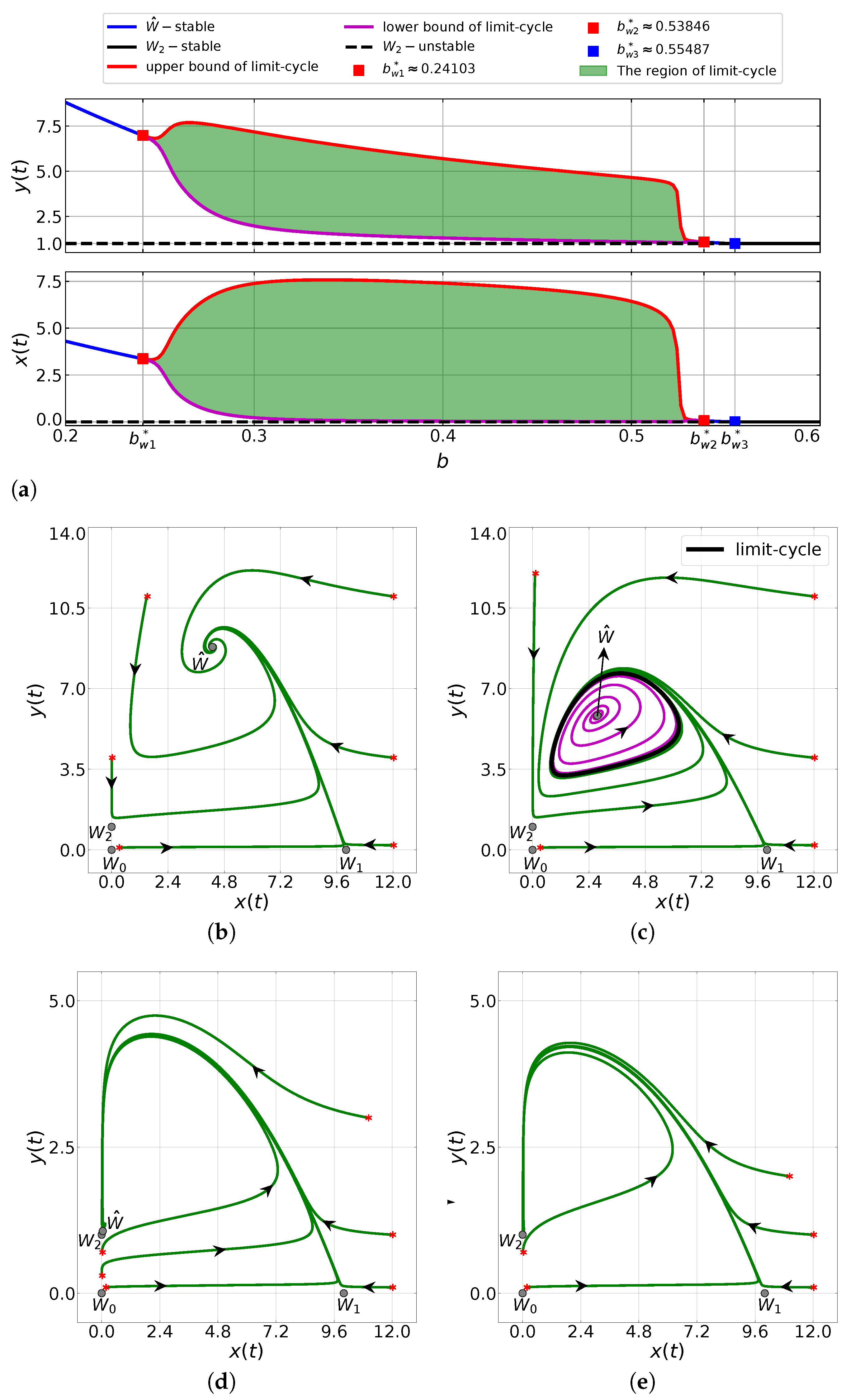
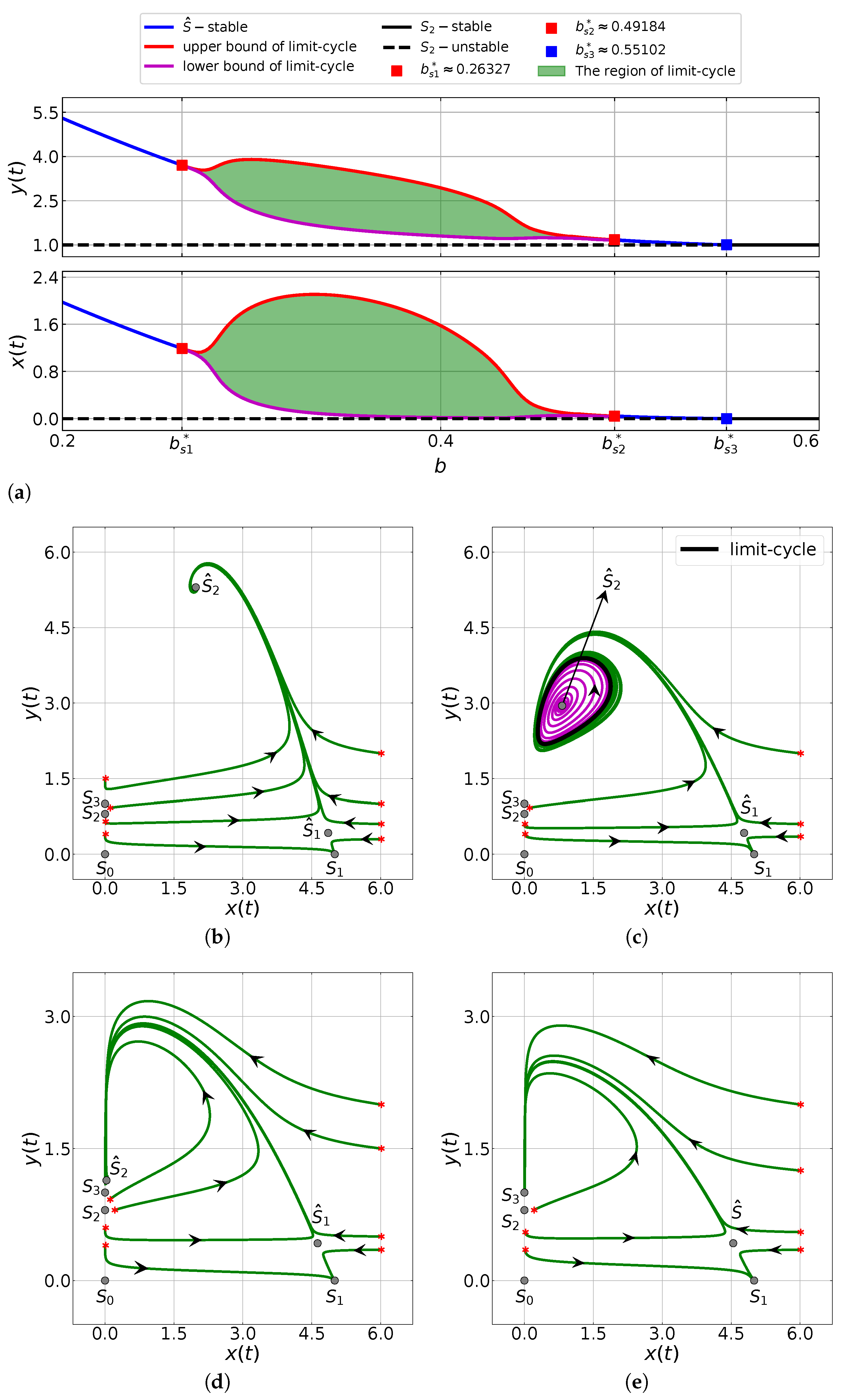
6.1. The Influence of the Capturing Rate $\left(b\right)$

To understand how the capturing rate $\left(b\right)$ could influence the dynamics of system (6) in the weak Allee effect case $(m<0)$, we use the following hypothetical parameter values.

$$\begin{array}{c}\hfill r=0.5,{\beta }_1=0.05,c=1,q=0.1,s=0.1,l=1,{\beta }_2=0.05,m=-1,\mathrm{and}n=3.\end{array}$$

(26)

The bifurcation diagrams for both predator and prey populations controlled by $b\in [0.2,0.6]$ and $\alpha =0.98$ are depicted in Figure 1a. When $b<b_{w1}^{*}\approx 0.24103$, the interior point $\widehat{W}$ is asymptotically stable. For example, we plot a phase portrait of the system (6) in Figure 1b for $b=0.20$. In this case, one can easily compute that ${\chi }_{1w}^2-4{\chi }_{2w}=-0.06299<0$ and ${\chi }_{1w}=-0.08727<0$. According to Theorem 4, the interior point $\widehat{W}=(4.30171,8.80734)$ is asymptotically stable. The stability of the interior point $\widehat{W}$ is also achieved in the interval $b\in (b_{w2}^{*}=0.53846,b_{w3}^{*}=0.55487)$. To show such typical behavior, we plot a phase portrait of the system (6) in Figure 1d for $b=0.54$. Furthermore, our numerical simulations also show the existence of limit-cycles solution enclosing the interior point $\widehat{W}$ for $b\in (b_{w1}^{*},b_{w2}^{*})$ as provided in the green area in Figure 1a. As an example, we plot some numerical solutions of the system (6) with $b=0.27$ in Figure 1c. It is observed that all solutions of system (6) converge to a limit-cycle and the interior point $\widehat{W}=(2.76631,5.82563)$ losses its stability. This situation shows that the system (6) undergoes a Hopf bifurcation with respect to b. When $b>b_{w3}^{*}$, the interior point $\widehat{W}$ does not exist anymore and the prey extinction point $W_2=(0,1)$ becomes stable via forward bifurcation. The numerical solutions of system (6), which show the stability of $W_2=(0,1)$, are shown in Figure 1e.

Next, we numerically investigate the effect of the capturing rate $\left(b\right)$ under the strong Allee effect case ($m>0$) using the following hypothetical parameters.

$$r=0.5,{\beta }_1=0.1,c=1,q=0.1,s=0.1,l=1,{\beta }_2=0.05,m=0.4,\mathrm{and}n=0.2.$$

(27)

Here, we also take $\alpha =0.98$. We notice that the predator extinction point $S_1=(5,0)$ is always asymptotically stable, see Theorem 5b. Then, by varying b from $0.2$ to $0.6$, we plot the bifurcation diagrams for both predator and prey population in Figure 2a. It is found that the system (6) in this case has similar qualitative behavior as in the previous simulation (see Figure 1 and Figure 2), with the exception of the stability properties of the predator extinction point $S_1=(5,0)$. In the first simulation, the predator extinction point is always unstable while, in the latter case, it is always locally asymptotically stable. The local stability properties of the predator extinction point can be clearly observed from the phase portraits depicted in Figure 2b–e.

Remark 1.

Based on Figure 1 and Figure 2, the capturing rate $\left(b\right)$ has great influence to both prey and predator population densities. For parameter values as in (26) and (27), for both weak and strong Allee effects, the densities of both prey and predator populations decrease with increasing capturing rates. In particular, increasing the capturing rate such that $b>b_{w3}^{*}$ (for the weak Allee effect case) or $b>b_{s3}^{*}$ (for the strong Allee effect case) may stabilize the prey extinction point $(0,1)$ as stated in Theorems 3c and 5c. This means that the prey population will become extinct while the predator still survives. We also notice that for the case of strong Allee effect $(m>0)$, the system (6) may exhibit a bistability phenomenon, see Figure 2b,d,e. Hence, the system (6) is highly sensitive to the initial condition when the Allee effect is strong. From the ecological point of view, this result is quite interesting. We can still maintain the existence of both prey and predator even under conditions of a strong Allee effect, that is, as long as we have a sufficiently large initial predator density. Furthermore, Figure 1b,d,e confirm the global asymptotic stability behavior of system (6) for the weak Allee effect case.

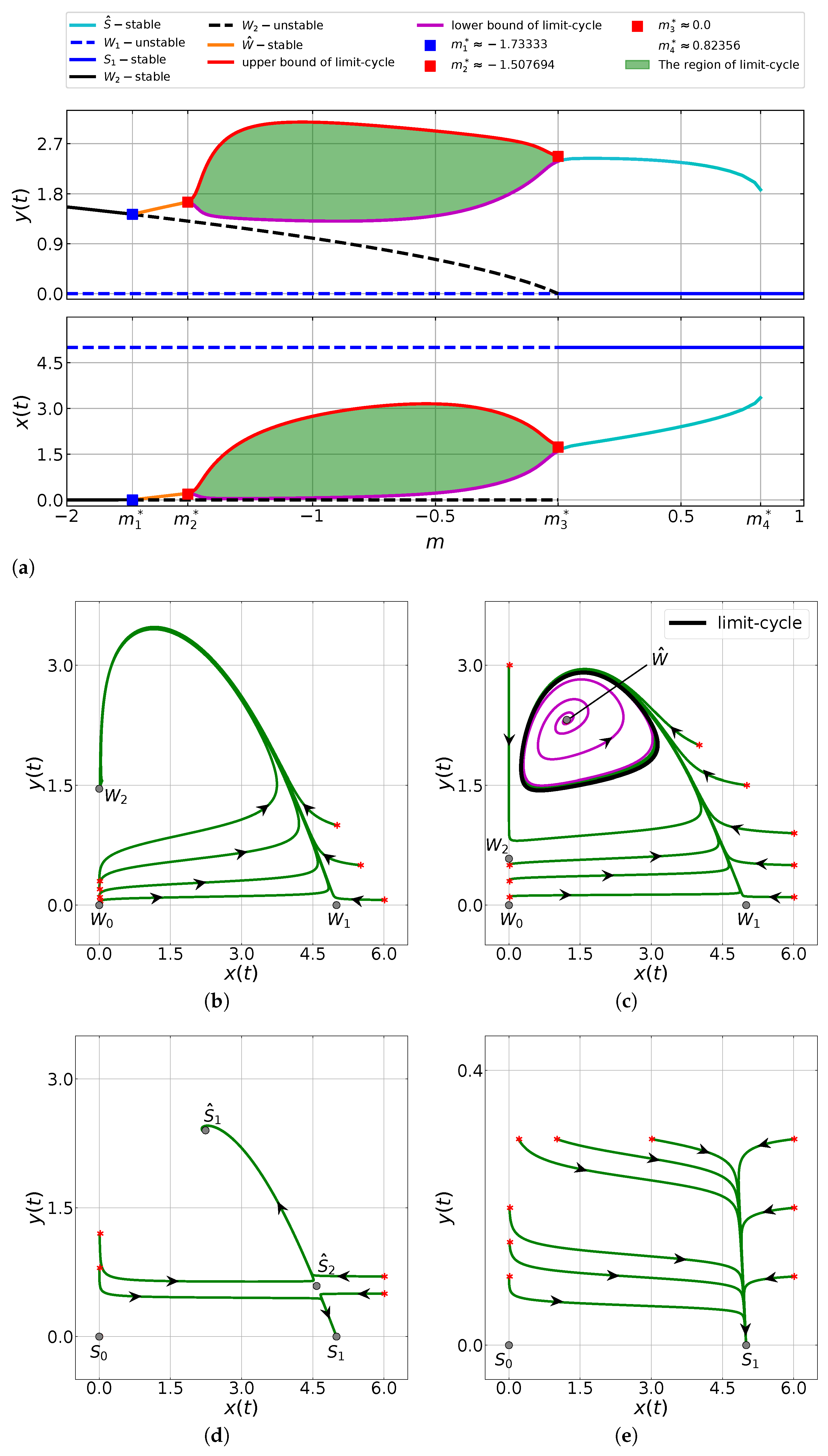
6.2. The Impacts of the Allee Threshold $\left(m\right)$

We next study numerically the impacts of the Allee threshold $\left(m\right)$ to the dynamics of system (6) using the following hypothetic values of parameters.

$$r=0.5,{\beta }_1=0.1,b=0.4,c=1,q=0.1,s=0.1,l=1,{\beta }_2=0.05,\mathrm{and}n=3.$$

(28)

In Figure 3a we show the bifurcation diagrams of both predator and prey populations for parameter $m\in [-2,1]$ and $\alpha =0.98$. It is shown that when $m<m_1^{*}\approx -1.73333$, the prey extinction point $W_2$ is asymptotically stable. If we increase m such that $m>m_1^{*}-1.73333$, then the prey extinction point $W_2$ loses its stability when an asymptotically stable interior point $\widehat{W}$ appears. This shows that the system (6) exhibits a forward bifurcation. The interior point $\widehat{W}$ remains asymptotically stable for $m\in (m_1^{*},m_2^{*})$. Moreover, Figure 3a shows the occurence of a Hopf bifurcation when m passes through $m_2^{*}\approx -1.50769$. Indeed, in the interval $m\in (m_2^{*},m_3^{*}=0)$, there is no stable equilibrium point and there exists a limit cycle around the interior point $\widehat{W}$; see the green area in Figure 3a. Our further observation shows that the system (6) with $m\in (m_3^{*},m_4^{*}\approx 0.82356)$ has a bistability phenomenon where both interior point $\widehat{S}$ and the predator extinction point $S_1=(5,0)$ are locally asymptotically stable. If we increase m such that $m>m_4^{*}$, the interior point $\widehat{S}$ loses its existence and the predator extinction point $S_1$ becomes a unique stable equilibrium point of the system (6).

In order to provide a better view of the dynamics of the system (6) with parameter values (28) and $\alpha =0.98$, we ploted several phase-portraits for different values of m in Figure 3b–e. Figure 3b shows the phase-portrait of the system (6) with $m=-1.79<m_1^{*}$. Here, we have $0.5=r<\frac{b{\overline{y}}_w}{1+q{\overline{y}}_w}=0.50960$ and $1.21=m+n<\frac{{\beta }_2}{ls}{({\overline{y}}_w+n)}^2=9.94580$. According to Theorem 3c, the prey extintion point $W_2=(0,1.46)$ is asymptotically stable. Figure 3b confirms this behavior where all numerical solutions converge to the prey extinction point $W_2=(0,1.46)$. The phase portrait of the system (6) with $m=-0.46>m_2^{*}$ is depicted in Figure 3c. In this respect, we have ${\chi }_{1w}=0.03488>0$ and $0.87258={\alpha }^{*}<\alpha =0.98$. Thus, the stability condition of the interior point $\widehat{W}=(1.21751,2.31593)$ in Figure 3c, where all numerical solutions of the system (6) are convergent to a limit-cycle. The appearence of a stable limit-cycle indicates the presence of a Hopf bifurcation in the system. Next, we consider a case of $m\in (m_3^{*},m_4^{*})$ by choosing $m=0.4$. The phase-portrait in Figure 3d shows that numerical solutions are convergent to the predator extinction point $S_1=(5,0)$ or to the interior point ${\widehat{S}}_1=(2.24039,2.40121)$, depending on the initial conditions. Hence, the system (6) exhibits a bistability phenomenon. Finally, if we take $m=0.90>m_4^{*}$, then we have situation where the interior point $\widehat{S}$ disappears and the predator extinction point $S_1=(5,0)$ becomes the only equilibrium point which is asymptotically stable. This behavior is plotted in Figure 3e.

Note that, when the Allee effect is weak, i.e., when $-n<m<0$, the predator always exists as depicted in the interval $[-2,m_3^{*}]$ in Figure 3a. In this case, the predator growth rate is always positive and the prey population could suffer from extinction as the m value decreases. On the other hand, when the Allee effect is strong, i.e., when $m>0$, there is a condition where the predator is always extinct as depicted by the blue solid line in the interval $[m_3^{*},1]$ in Figure 3a. However, generally speaking, the system (6) could have a positive or negative growth rate on the predator population since there is a bistability phenomenon in that interval as explained before. These situations show that our system (6) may provide the condition for the existence of the predator population which is affected by the double Allee effect.

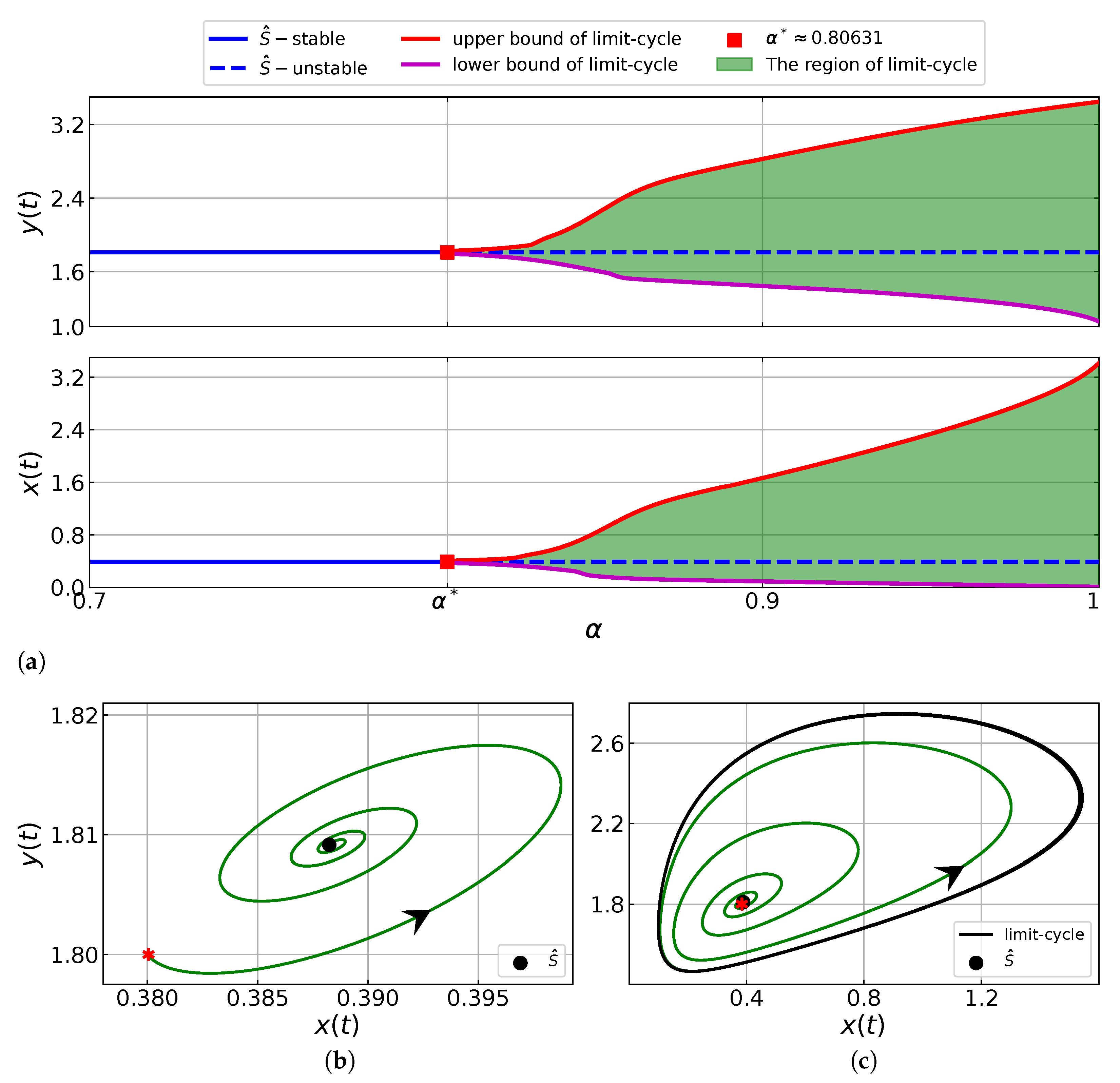
6.3. The Effects of the Order of Fractional System $\left(\alpha \right)$

In the following simulations, we study the influence of the order of the fractional derivative $\left(\alpha \right)$ by considering the system (6) with the following hypothetical parameter values.

$$\begin{array}{ccccccccccccccc}r& =& 0.5,\hfill & {\beta }_1& =& 0.1,\hfill & b& =& 0.4,\hfill & c& =& 1,\hfill & q& =& 0.1,\hfill \\ s& =& 0.1,\hfill & l& =& 1,\hfill & {\beta }_2& =& 0.05,\hfill & m& =& 0.5,\hfill & n& =& 0.2.\hfill \end{array}$$

(29)

Based on parameter values (29) and Theorem 7, we can find a critical value ${\alpha }^{*}\approx 0.80631$ such that the interior point is asymptotically stable if $\alpha <{\alpha }^{*}$ and it is unstable if $\alpha >{\alpha }^{*}$. In order to observe such behavior, we plot the bifurcation diagram for $\alpha \in [0.7,1.0]$, see Figure 4a. It is observed that the interior point $\widehat{S}=(0.38825,1.80915)$ is asymptotically stable when $\alpha <{\alpha }^{*}$. If $\alpha >{\alpha }^{*}$, then the interior point $\widehat{S}$ loses its stability and all numerical solutions converge to a limit-cycle via a Hopf bifurcation. The Hopf bifurcation can also be observed from the phase-portraits shown in Figure 4b for $\alpha =0.73<{\alpha }^{*}$ and Figure 4c for $\alpha =0.89>{\alpha }^{*}$.

In Figure 4a, we observe that the order of the fractional derivative does not affect the stability of the interior point as long as $0<\alpha <{\alpha }^{*}$. To verify this property, we plot in Figure 5 the time series of both prey and predator populations for $\alpha =0.5,0.6,0.7,0.75$. It is shown that all solutions are indeed convergent to the interior point $\widehat{S}=(0.38825,1.80915)$, but the solution of system (6) with a higher–order fractional derivative has faster convergence.

7. Conclusions

In this paper, a fractional-order Leslie–Gower predator-prey model with Beddington–DeAngelis functional response and double Allee effect in the predator population is proposed and the dynamics of the model has been analyzed. First, the existence, uniqueness, non-negativity, and boundedness of the solution have been proven. We then determined all possible non-negative equilibrium points and their local and global stability properties. We found that the model has four types of biologically feasible equilibrium. The extinction of both prey and predator point is always unstable for both weak and strong Allee effect cases. The predator extinction point is always stable for the strong Allee effect case, but it is always unstable for the weak Allee effect case. The prey extinction point and the interior point are conditionally stable. Our numerical simulations showed that for the case of the weak Allee effect, there is a capturing rate threshold $b^{*}$ such that for $b>b^{*}$ the prey population is extinct while the predator population still survives. However, for the case of the strong Allee effect, the situation is also dependent on the initial value. Here, if the initial predator population is relatively low then the predator will become extinct but the prey will survive. Additionally, we also proved the existence of a Hopf bifurcation about the interior point driven by the order of the fractional derivative $\left(\alpha \right)$ and the critical ${\alpha }^{*}$ of this bifurcation has been determined analytically. The occurrence of the Hopf bifurcation has been confirmed by our numerical simulations. The existence of Hopf bifurcation controlled by $\alpha$ has also been observed in [31,32]. This shows that the unstable interior point of the first order system (i.e., the system is convergent to a limit cycle) may become stable in the fractional order system (i.e., the system converges to the interior point).

References

1. Cushing, J.M. Backward bifurcations and strong Allee effects in matrix models for the dynamics of structured populations. J. Biol. Dyn. 2014, 8, 57–73. [Google Scholar] [CrossRef] [Green Version]
2. Buffoni, G.; Groppi, M.; Soresina, C. Dynamics of predator-prey models with a strong Allee effect on the prey and predator-dependent trophic functions. Nonlinear Anal. Real World Appl. 2016, 30, 143–169. [Google Scholar] [CrossRef]
3. Sasmal, S.K.; Chattopadhyay, J. An eco-epidemiological system with infected prey and predator subject to the weak Allee effect. Math. Biosci. 2013, 246, 260–271. [Google Scholar] [CrossRef]
4. Saifuddin, M.; Biswas, S.; Samanta, S.; Sarkar, S.; Chattopadhyay, J. Complex dynamics of an eco-epidemiological model with different competition coefficients and weak Allee in the predator. Chaos Solitons Fractals 2016, 91, 270–285. [Google Scholar] [CrossRef]
5. Pal, S.; Sasmal, S.K.; Pal, N. Chaos control in a discrete-time predator-prey model with weak Allee effect. Int. J. Biomath. 2018, 11, 1–26. [Google Scholar] [CrossRef]
6. Arancibia-Ibarra, C.; Flores, J.; Bode, M.; Pettet, G.; Van Heijster, P. A modified May–Holling–Tanner predator-prey model with multiple Allee effects on the prey and an alternative food source for the predator. Discret. Contin. Dyn. Syst. 2021, 26, 943–962. [Google Scholar] [CrossRef]
7. Berec, L.; Angulo, E.; Courchamp, F. Multiple Allee effects and population management. Trends Ecol. Evol. 2007, 22, 185–191. [Google Scholar] [CrossRef]
8. Pavlová, V.; Berec, L.; Boukal, D.S. Caught between two Allee effects: Trade-off between reproduction and predation risk. J. Theor. Biol. 2010, 264, 787–798. [Google Scholar] [CrossRef] [PubMed] [Green Version]
9. Feng, P.; Kang, Y. Dynamics of a modified Leslie–Gower model with double Allee effects. Nonlinear Dyn. 2015, 80, 1051–1062. [Google Scholar] [CrossRef]
10. Lai, L.; Zhu, Z.; Chen, F. Stability and bifurcation in a predator–prey model with the additive Allee effect and the fear effect. Mathematics 2020, 8, 1280. [Google Scholar] [CrossRef]
11. Martínez-Jeraldo, N.; Aguirre, P. Allee effect acting on the prey species in a Leslie–Gower predation model. Nonlinear Anal. Real World Appl. 2019, 45, 895–917. [Google Scholar] [CrossRef]
12. Zhang, C.; Yang, W. Dynamic behaviors of a predator–prey model with weak additive Allee effect on prey. Nonlinear Anal. Real World Appl. 2020, 55, 103137. [Google Scholar] [CrossRef]
13. Xiao, Z.; Xie, X.; Xue, Y. Stability and bifurcation in a Holling type II predator–prey model with Allee effect and time delay. Adv. Differ. Equ. 2018, 2018, 288. [Google Scholar] [CrossRef]
14. Teixeira Alves, M.; Hilker, F.M. Hunting cooperation and Allee effects in predators. J. Theor. Biol. 2017, 419, 13–22. [Google Scholar] [CrossRef]
15. Guan, X.; Liu, Y.U.; Xie, X. Stability analysis of a Lotka-Volterra type predator-prey system with Allee effect on the predator species. Commun. Math. Biol. Neurosci. 2018, 2018, 9. [Google Scholar] [CrossRef]
16. Bodine, E.N.; Yust, A.E. Predator–prey dynamics with intraspecific competition and an Allee effect in the predator population. Lett. Biomath. 2017, 4, 23–38. [Google Scholar] [CrossRef]
17. Pal, P.J.; Saha, T. Qualitative analysis of a predator-prey system with double Allee effect in prey. Chaos Solitons Fractals 2015, 73, 36–63. [Google Scholar] [CrossRef]
18. Singh, M.K.; Bhadauria, B.S.; Singh, B.K. Bifurcation analysis of modified Leslie-Gower predator-prey model with double Allee effect. Ain Shams Eng. J. 2018, 9, 1263–1277. [Google Scholar] [CrossRef] [Green Version]
19. Courchamp, F.; Clutton-Brock, T.; Grenfell, B. Multipack dynamics and the Allee effect in the African wild dog, Lycaon pictus. Anim. Conserv. 2000, 3, 277–285. [Google Scholar] [CrossRef]
20. El-Shahed, M.; Ahmed, A.M.; Abdelstar, I.M.E. Dynamics of a plant-herbivore model with fractional order. Progr. Fract. Differ. Appl. 2017, 3, 59–67. [Google Scholar] [CrossRef]
21. Suryanto, A.; Darti, I.; Panigoro, H.S.; Kilicman, A. A fractional-order predator–prey model with ratio-dependent functional response and linear harvesting. Mathematics 2019, 7, 1100. [Google Scholar] [CrossRef] [Green Version]
22. Khoshsiar Ghaziani, R.; Alidousti, J.; Eshkaftaki, A.B. Stability and dynamics of a fractional order Leslie–Gower prey–predator model. Appl. Math. Model. 2016, 40, 2075–2086. [Google Scholar] [CrossRef]
23. Panigoro, H.S.; Suryanto, A.; Kusumawinahyu, W.M.; Darti, I. Continuous threshold harvesting in a Gause-type predator-prey model with fractional-order. AIP Conf. Proc. 2020, 2264, 040001. [Google Scholar] [CrossRef]
24. Panigoro, H.S.; Suryanto, A.; Kusumawinahyu, W.M.; Darti, I. Dynamics of an eco-epidemic predator–prey model involving fractional derivatives with power-law and Mittag–Leffler kernel. Symmetry 2021, 13, 785. [Google Scholar] [CrossRef]
25. Petras, I. Fractional-Order Nonlinear Systems; Springer: London, UK, 2011. [Google Scholar]
26. Kumar, S.; Kumar, R.; Cattani, C.; Samet, B. Chaotic behaviour of fractional predator-prey dynamical system. Chaos Solitons Fractals 2020, 135, 109811. [Google Scholar] [CrossRef]
27. Singh, J.; Ganbari, B.; Kumar, D.; Baleanu, D. Analysis of fractional model of guava for biological pest control with memory effect. J. Adv. Res. 2021, in press. [Google Scholar] [CrossRef]
28. El-Ajou, A.; Al-Smadi, M.; Oqielat, M.N.; Momani, S.; Hadid, S. Smooth expansion to solve high-order linear conformable fractional PDEs via residual power series method: Applications to physical and engineering equations. Ain Shams Eng. J. 2020, 11, 1243–1254. [Google Scholar] [CrossRef]
29. Ali, H.M.; Habib, M.A.; Miah, M.M.; Akbar, M.A. Solitary wave solutions to some nonlinear fractional evolution equations in mathematical physics. Heliyon 2020, 6, e03727. [Google Scholar] [CrossRef] [PubMed]
30. Shi, G.; Gao, J. European option pricing problems with fractional uncertain processes. Chaos Solitons Fractals 2021, 143, 110606. [Google Scholar] [CrossRef]
31. Suryanto, A.; Darti, I.; Anam, S. Stability analysis of a fractional order modified Leslie-Gower model with additive Allee effect. Int. J. Math. Math. Sci. 2017, 2017, 8273430. [Google Scholar] [CrossRef] [Green Version]
32. Baisad, K.; Moonchai, S. Analysis of stability and Hopf bifurcation in a fractional Gauss-type predator–prey model with Allee effect and Holling type-III functional response. Adv. Differ. Equ. 2018, 2018, 82. [Google Scholar] [CrossRef] [Green Version]
33. Indrajaya, D.; Suryanto, A.; Alghofari, A.R. Dynamics of modified Leslie-Gower predator-prey model with Beddington-DeAngelis functional response and additive Allee effect. Int. J. Ecol. Dev. 2016, 31, 60–71. [Google Scholar]
34. Ginzburg, L.R. Assuming reproduction to be a function of consumption raises doubts about some popular predator-prey models. J. Anim. Ecol. 1998, 67, 325–327. [Google Scholar] [CrossRef]
35. Leslie, P.H.; Gower, J.C. The properties of a stochastic model for the predator-prey type of interaction between two species. Biometrika 1960, 47, 219–234. [Google Scholar] [CrossRef]
36. Mallet, J. The struggle for existence: How the notion of carrying capacity, K, obscures the links between demography, Darwinian evolution, and speciation. Evol. Ecol. Res 2012, 14, 627–665. [Google Scholar]
37. Gabriel, J.P.; Saucy, F.; Bersier, L.-F. Paradoxes in the logistic equation? Ecol. Model. 2005, 185, 147–151. [Google Scholar] [CrossRef] [Green Version]
38. Arditi, R.; Bersier, L.-F.; Rohr, R.P. The perfect mixing paradox and the logistic equation: Verhulst vs. Lotka. Ecosphere 2016, 7, e01599. [Google Scholar] [CrossRef] [Green Version]
39. Aziz-Alaoui, M.A.; Okiye, M.D. Boundedness and Global Stability for a Predator-Prey Model with Modified and Holling-Type II Schemes. Appl. Math. Lett. 2002, 16, 1069–1075. [Google Scholar] [CrossRef] [Green Version]
40. Yu, S. Global stability of a modified Leslie-Gower model with Beddington-DeAngelis functional response. Adv. Differ. Equ. 2014, 2014, 84. [Google Scholar] [CrossRef] [Green Version]
41. Vera-Damián, Y.; Vidal, C.; González-Olivares, E. Dynamics and bifurcations of a modified Leslie-Gower–type model considering a Beddington-DeAngelis functional response. Math. Methods Appl. Sci. 2019, 42, 3179–3210. [Google Scholar] [CrossRef]
42. Melese, D.; Feyissa, S. Stability and bifurcation analysis of a diffusive modified Leslie-Gower prey-predator model with prey infection and Beddington DeAngelis functional response. Heliyon 2021, 7, e06193. [Google Scholar] [CrossRef]
43. Arancibia-Ibarra, C.; Flores, J. Dynamics of a Leslie–Gower predator–prey model with Holling type II functional response, Allee effect and a generalist predator. Math. Comput. Simul. 2021, 188, 1–22. [Google Scholar] [CrossRef]
44. Tiwari, B.; Raw, S.N. Dynamics of Leslie–Gower model with double Allee effect on prey and mutual interference among predators. Nonlinear Dyn. 2021, 1229–1257, 1229–1257. [Google Scholar] [CrossRef]
45. Zhou, S.R.; Liu, Y.F.; Wang, G. The stability of predator–prey systems subject to the Allee effects. Theor. Popul. Biol. 2005, 67, 23–31. [Google Scholar] [CrossRef]
46. Diethelm, K. A fractional calculus based model for the simulation of an outbreak of dengue fever. Nonlinear Dyn. 2013, 71, 613–619. [Google Scholar] [CrossRef]
47. Moustafa, M.; Mohd, M.H.; Ismail, A.I.; Abdullah, F.A. Dynamical analysis of a fractional-order eco-epidemiological model with disease in prey population. Adv. Differ. Equ. 2020, 2020, 48. [Google Scholar] [CrossRef]
48. Panigoro, H.S.; Suryanto, A.; Kusumawinahyu, W.M.; Darti, I. A Rosenzweig–MacArthur model with continuous threshold harvesting in predator involving fractional derivatives with power law and mittag–leffler kernel. Axioms 2020, 9, 122. [Google Scholar] [CrossRef]
49. Rahmi, E.; Darti, I.; Suryanto, A.; Trisilowati; Panigoro, H.S. Stability analysis of a fractional-order Leslie-Gower model with Allee effect in predator. J. Phys. Conf. Ser. 2021, 1821, 012051. [Google Scholar] [CrossRef]
50. Li, Y.; Chen, Y.Q.; Podlubny, I. Stability of fractional-order nonlinear dynamic systems: Lyapunov direct method and generalized Mittag-Leffler stability. Comput. Math. Appl. 2010, 59, 1810–1821. [Google Scholar] [CrossRef] [Green Version]
51. Li, H.L.; Zhang, L.; Hu, C.; Jiang, Y.L.; Teng, Z. Dynamical analysis of a fractional-order predator-prey model incorporating a prey refuge. J. Appl. Math. Comput. 2017, 54, 435–449. [Google Scholar] [CrossRef]
52. Ahmed, E.; El-Sayed, A.; El-Saka, H.A. On some Routh–Hurwitz conditions for fractional order differential equations and their applications in Lorenz, Rössler, Chua and Chen systems. Phys. Lett. A 2006, 358, 1–4. [Google Scholar] [CrossRef]
53. Li, X.; Wu, R. Hopf bifurcation analysis of a new commensurate fractional-order hyperchaotic system. Nonlinear Dyn. 2014, 78, 279–288. [Google Scholar] [CrossRef]
54. Vargas-De-León, C. Volterra-type Lyapunov functions for fractional-order epidemic systems. Commun. Nonlinear. Sci. Numer. Simul. 2015, 24, 75–85. [Google Scholar] [CrossRef]
55. Huo, J.; Zhao, H.; Zhu, L. The effect of vaccines on backward bifurcation in a fractional order HIV model. Nonlinear Anal. Real World Appl. 2015, 26, 289–305. [Google Scholar] [CrossRef]
56. Arenas, A.J.; González-Parra, G.; Chen-Charpentier, B.M. Construction of nonstandard finite difference schemes for the SI and SIR epidemic models of fractional order. Math. Comput. Simul 2016, 121, 48–63. [Google Scholar] [CrossRef]
57. Barman, D.; Roy, J.; Alrabaiah, H.; Panja, P.; Mondal, S.P.; Alam, S. Impact of predator incited fear and prey refuge in a fractional order prey predator model. Chaos Solitons Fractals 2020, 142, 110420. [Google Scholar] [CrossRef]
58. Das, M.; Samanta, G.P. A prey-predator fractional order model with fear effect and group defense. Int. J. Dyn. Control 2020, 9, 334–349. [Google Scholar] [CrossRef]
59. Alidousti, J.; Ghafari, E. Dynamic behavior of a fractional order prey-predator model with group defense. Chaos Solitons Fractals 2020, 134, 109688. [Google Scholar] [CrossRef]
60. Jena, R.M.; Chakraverty, S.; Baleanu, D.; Jena, S.K. Analysis of time-fractional dynamical model of romantic and interpersonal relationships with non-singular kernels: A comparative study. Math. Meth. Appl. Sci. 2020, 44, 2183–2199. [Google Scholar] [CrossRef]
61. Ullah, I.; Ahmad, S.; Rahman, M.; Arfan, M. Investigation of fractional order tuberculosis (TB) model via Caputo derivative. Chaos Solitons Fractals 2020, 142, 110479. [Google Scholar] [CrossRef]
62. Mahmood, S.; Shah, R.; Khan, H.; Arif, M. Laplace adomian decomposition method for multi dimensional time fractional model of Navier-Stokes equation. Symmetry 2019, 11, 149. [Google Scholar] [CrossRef] [Green Version]
63. Diethelm, K.; Ford, N.J.; Freed, A.D. A predictor-corrector approach for the numerical solution of fractional differential equations. Nonlinear Dyn. 2002, 29, 3–22. [Google Scholar] [CrossRef]
Figure 1. Dynamics of system (6) with parameter values (26) and α = 0.98 . (a) Bifurcation diagram of system (6) driven by b for the case of the weak Allee effect ( m = 1 < 0 ) . (be) Phase-portrait of system (6) with (b) b = 0.20 , (c) b = 0.27 , (d) b = 0.54 , and (e) b = 0.57 . The predator extinction point is always unstable.
Fractalfract 05 00084 g001
Figure 2. Dynamics of system (6) with parameter values (27) and α = 0.98 . (a) Bifurcation diagram of system (6) driven by b for the case of strong Allee effect ( m = 0.4 > 0 ) . (be) Phase-portrait of system (6) with (b) b = 0.20 , (c) b = 0.40 , (d) b = 0.50 , and (e) b = 0.60 . The predator extinction point is always locally stable.
Fractalfract 05 00084 g002
Figure 3. Dynamics of system (6) with parameter values (28) and α = 0.98 . (a) Bifurcation diagram of system (6) driven by m. (be) Phase-portrait of system (6) with (b) m = 1.79 , (c) m = 0.46 , (d) m = 0.40 , and (e) m = 0.90 . The predator extinction point is unstable for the weak Allee effect case ( m < 0 ) and is locally asymptotically stable for the strong Allee effect case ( m < 0 ) .
Fractalfract 05 00084 g003
Figure 4. Dynamics of system (6) with parameter values (29). (a) Bifurcation diagram of system (6) driven by α . (b,c) Phase-portrait of system (6) with (b) α = 0.73 and (c) α = 0.89 .
Fractalfract 05 00084 g004
Figure 5. Time series of system (6) with parameter values (29) and the initial conditions taken around the interior point S ^ = ( 0.38825 , 1.80915 ) .
Fractalfract 05 00084 g005
Publisher’s Note: MDPI stays neutral with regard to jurisdictional claims in published maps and institutional affiliations.