Article

A Numerical Study of Nonlinear Fractional Order Partial Integro-Differential Equation with a Weakly Singular Kernel

1
School of Mathematical Sciences, Universiti Sains Malaysia, Penang 11800, Malaysia
2
School of Engineering, Monash University Malaysia, Selangor 47500, Malaysia
3
Department of Mathematics, University of Malakand, Dir(L), Khyber Pakhtunkhwa 18000, Pakistan
4
Center of Excellence in Theoretical and Computational Science (TaCS-CoE) & KMUTTFixed Point Research Laboratory, Room SCL 802 Fixed Point Laboratory, Science Laboratory Building, Departments of Mathematics, Faculty of Science, King Mongkut’s University of Technology Thonburi (KMUTT), 126 Pracha-Uthit Road, Bang Mod, Thung Khru, Bangkok 10140, Thailand
5
Department of Medical Research, China Medical University Hospital, China Medical University, Taichung 40402, Taiwan
*
Author to whom correspondence should be addressed.
Fractal Fract. 2021, 5(3), 85; https://doi.org/10.3390/fractalfract5030085
Submission received: 12 July 2021 / Revised: 25 July 2021 / Accepted: 26 July 2021 / Published: 2 August 2021
(This article belongs to the Special Issue Novel Numerical Solutions of Fractional PDEs)

Abstract

:
Fractional differential equations can present the physical pathways with the storage and inherited properties due to the memory factor of fractional order. The purpose of this work is to interpret the collocation approach for tackling the fractional partial integro-differential equation (FPIDE) by employing the extended cubic B-spline (ECBS). To determine the time approximation, we utilize the Caputo approach. The stability and convergence analysis have also been analyzed. The efficiency and reliability of the suggested technique are demonstrated by two numerical applications, which support the theoretical results and the effectiveness of the implemented algorithm.

1. Introduction

Fractional calculus (FC) has explored the concept of differentiation and integration to non-integer order. FC is a more generalized version of classical calculus. FC is as old as classical calculus, but it is gaining popularity these days because of the implementations in many domains like science and engineering. Fractional partial differential equations (FPDEs) have gained much popularity because of their exceptional simulation properties in various scientific areas. It has been used to represent physical and technical phenomena that are described tremendously by fractional differential equations. The fractional derivative models are used to recognize better those systems, which required accurate modeling of damping, non-Fourier heat conduction, acoustic dissipation, geophysics, relaxation, creep, viscoelasticity, rheology, and fluid dynamics, Malaria and COVID-19 [1,2,3,4].
Integro-differential equations of fractional order are the type of models that include both integro-differential equations and fractional derivatives. The analysis of partial integro-differential equations with fractional specifications is an important element of the theory and implementations of FC, which have considered crucial mathematical methods for describing and analysing a broad variety of actual challenges in natural science, technology, and engineering [5,6,7,8]. The mathematical models of physical phenomena and their implementations in heat conduction [9], reactor dynamics [10], flow in fractured bio-materials [11], electricity swaption [12], visco-elasticity [13], population dynamics, convection diffusion [14] and grain growth [15]. In this study, we will look at the nonlinear FPIDE [16]:
0 C D t γ V ( y , t ) + V V y = 0 t ( t s ) α 1 V y y ( y , s ) d s + G ( y , t ) , 0 < y < L , 0 < t < T ,
with initial condition
V ( y , 0 ) = f ( y ) , 0 y L ,
and boundary conditions
V ( 0 , t ) = V ( L , T ) = 0 , 0 t T ,
where γ , α ( 0 , 1 ) , T , L are positive constants, and G ( y , t ) , f ( y ) are given functions. 0 C D t γ denotes the Caputo fractional derivative (CFD) and is interpreted as
0 C D t γ F ( y ) = 1 Γ ( n γ ) 0 y ( y ξ ) n 1 γ F ( n ) ( ξ ) d ξ , n 1 < γ n , n N , F ( n ) ( y ) , γ = n .
where Γ is the Euler’s Gamma function.
At various stages of real systems, fractional derivatives and integral operators are more suitable than standard derivatives and integration, which provide a more precise explanation of structural and genetic features of several dynamical and physical procedures. As a result, accurate computational methods are used to approximately cope with the complexities of fractional derivatives contained in such equations. These complexities are due to the possibility of the singularities of the kernels causing drastic fluctuations in the solution. Consequently, it isn’t easy to acquire a closed-form solution in several implementations, particularly in nonlinear scenarios, so an approximation of physical description is needed. Alternatively, many studies have been conducted to investigate the presence of a unique solution to fractional order integro-differential equations, such as Hu et al. [17], Li et al. [18], Karthikeyan and Trujillo [19], Chuong et al. [20].
The majority of FPIDE cannot be addressed exact analytically, finding more effective approximate approaches using computational methods would be extremely beneficial. Several authors have focused their attention on searching and exploring solutions of the Fractional partial intego-differential equations (FPIDEs) using various analytical and numerical strategies. Awawdeh et al. [21] utilized the homotopy analysis approximation to solve the linear FPIDE analytically. Hussain et al. [22] solved the FPIDE analytically by the variation iteration method. Mittal and Nigam [23] implemented the Adomian decomposition method to handle the FPIDE. Rawashdeh [24] suggested a collocation approach for solving the FPIDE numerically by the polynomial spline. Eslahchi et al. [25] developed the jacobi technique to solve nonlinear FPIDE, also analyzed stability and convergence. Zhao et al. [26] employed piecewise polynomial collocation approaches to tackle FPIDEs containing weakly singular kernels. Arshed [27] demonstrated the B-spline technique for solving linear FPIDE. Unhale and Kendre [28] presented collocation technique to solve the nonlinear FPIDE utilizing the Chebyshev polynomials and the shifted Legendre polynomials. Avazzadeh et al. [29] established a hybrid technique by blending the Legendre wavelets, and operational matrix of fractional integration. A numerical technique based on Legendre-Laguerre and the collocation method has been considered by Dehestani et al. [30].
The B-spline was proposed by many authors to solve fractional partial differential models [31,32,33,34,35,36,37,38]. These functions can adjust every point in the domain and approximate the solution with maximum frequency accuracy. For solving FPDEs, a variety of numerical approaches have already been developed. However, so far as we know, no such research on the utilization of B-splines exists in solving the nonlinear FPIDE. Therefore, we intend to fill this gap. We aim to extend the ECBS technique for the solution of the nonlinear FPIDE model with a weakly singular kernel. The article is partitioned as follows: In Section 2, the basis functions and the time approximation are presented. In Section 3, a derivation of the method is described. The stability and convergence of recommended technique are analyzed in Section 4. Two applications and discussions are shown in Section 5. Finally, the results of the recommended technique are displayed in Section 6.

2. Preliminaries

Definition 1.
Let { y i } be an evenly distributed splitting of a finite domain for i Z . As a result, the proposed interval is segregated into M equivalent subparts at the connections as y i = y 0 + i h , where h is the moving scale. The ECBS functions at the y i over the proposed interval are shown below [39]:
B i ( y , ρ ) = 1 24 h 4 4 h ( 1 ρ ) ( y y i 2 ) 3 + 3 ρ ( y y i 2 ) 4 , y [ y i 2 , y i 1 ) , ( 4 ρ ) h 4 + 12 h 3 ( y y i 1 ) + 6 h 2 ( 2 + ρ ) ( y y i 1 ) 2 12 h ( y y i 1 ) 3 3 ρ ( y y i 1 ) 4 , y [ y i 1 , y i ) , ( 4 ρ ) h 4 + 12 h 3 ( y i + 1 y ) + 6 h 2 ( 2 + ρ ) ( y i + 1 y ) 2 12 h ( y i + 1 y ) 3 3 ρ ( y i + 1 y ) 4 , y [ y i , y i + 1 ) , 4 h ( 1 ρ ) ( y i + 2 y ) 3 + 3 ρ ( y i + 2 y ) 4 , y [ y i + 1 , y i + 2 ) , 0 , otherwise ,
where i = 1 ( 1 ) M + 1 , ρ R is a free parameter in the interval [ 8 , 1 ] and y R is a variable. The cubic B-spline and ECBS basis have identical characteristics for ρ [ 8 , 1 ] . For ρ = 0 , the ECBS converts to cubic B-spline. There is a unique V ^ ( y , t ) , that preserves the specified conditions, so that
v ( y , t ) = i = 1 M + 1 η i ( t ) E i ( y , ρ ) .
The following are the V ^ ( y , t ) , V ^ ( y , t ) and V ^ ( y , t ) at the edges:
V ^ ( y i , t ) = σ 1 η i 1 ( t ) + σ 2 η i ( t ) + σ 1 η i + 1 ( t ) , V ^ ( y i , t ) = σ 3 η i 1 ( t ) + σ 3 η i + 1 ( t ) , V ^ ( y i , t ) = σ 4 η i 1 ( t ) + σ 5 η i ( t ) + σ 4 η i + 1 ( t ) ,
where σ 1 = 4 ρ 24 , σ 2 = 8 + ρ 12 , σ 3 = 1 2 h , σ 4 = 2 + ρ 2 h 2 , σ 5 = 2 + ρ h 2 .

Temporal Approximation

Let t q = q τ , q = 0 , 1 , , Q , while τ = T Q is a time moving scale. The CFD approximation in the form of difference technique can be interpreted as
0 C D t γ V ( y , t p + 1 ) = 1 Γ ( 2 γ ) p = 0 q b p γ V ( y , t q p + 1 ) V ( y , t q p ) τ γ + D q + 1 ,
| D q + 1 | D 1 τ 2 γ ,
where D 1 is a constant and b p = ( p + 1 ) 1 γ p 1 γ . The integral expression of Equation (1) can be explained as:
0 t ( t q + 1 , s ) α 1 V y y ( y , s ) d s = 0 t q + 1 s α 1 V y y ( y , t q + 1 s ) d s , = p = 0 q t p t p + 1 s α 1 V y y ( y , t q + 1 s ) d s , = p = 0 q V y y ( y , t q p + 1 ) t p t p + 1 s α 1 d s ,
0 t ( t q + 1 , s ) α 1 V y y ( y , s ) d s = τ α α p = 0 q V y y ( y , t q p + 1 ) [ ( p + 1 ) α p α ] = τ α α p = 0 q V y y ( y , t q p + 1 ) b p α .
Lemma 1.
The b p s assure the following constrains [40]:
  • b 0 γ = 1 , b 0 α = 1 .
  • b 0 γ > b 1 γ > b 2 γ > > b p γ , and b 0 α > b 1 α > b 2 α > > b p α , b p α , b p γ 0 as p .
  • b p γ , b p α > 0 for p = 0 , 1 , , q .
  • p = 0 q ( b p γ b p + 1 γ ) + b q + 1 γ = ( 1 b 1 γ ) + p = 1 q 1 ( b p γ b p + 1 γ ) + b q γ = 1 .
  • p = 0 q b p α > 1 .
Proof. All parts can be easily verified.
p = 0 q b p α = p = 0 q [ ( p + 1 ) α p α ] = ( 1 α 0 ) + ( 2 α 1 α ) + ( 3 α 2 α ) + + ( ( q + 1 ) α q α ) = ( q + 1 ) α > 1 , f o r q 1 .

3. Derivation of the Procedure

We employ the ECBS and the CFD to address the proposed model. By plugging Equations (8) and (10) in (1), we obtain
τ γ Γ ( 2 γ ) p = 0 q b p γ [ V q p + 1 V q p ] + ( V V y ) q + 1 = τ α α p = 0 q V y y q p + 1 b p α + G q + 1 .
Linearize the non-linear term as [41]:
( V V y ) q + 1 = V q + 1 V y q + V q V y q + 1 ( V V y ) q .
By plugging Equation ( 12 ) into ( 11 ) , we have
τ γ Γ ( 2 γ ) p = 0 q b p γ [ V q p + 1 V q p ] + V q + 1 V y q + V q V y q + 1 ( V V y ) q = τ α α p = 0 q V y y q p + 1 b p α + G q + 1 .
Using expression ( 6 ) in the above equation, we obtain
τ γ Γ ( 2 γ ) p = 0 q b p γ i = 1 M + 1 η i q p + 1 E i i = 1 M + 1 η i q p E i + i = 1 M + 1 η i q + 1 E i i = 1 M + 1 η i q E i + i = 1 M + 1 η i q E i i = 1 M + 1 η i q + 1 E i i = 1 M + 1 η i q E i i = 1 M + 1 η i q E i = τ α α p = 0 q b p α i = 1 M + 1 η i q p + 1 E i + G q + 1 .
After some computation in the above expression, we get
V ^ q + 1 + r V ^ q V ^ y q + 1 + r V ^ q + 1 V ^ y q r r 1 V ^ y y q + 1 = b q γ V ^ 0 + r V ^ q V ^ y q + p = 0 q 1 ( b q γ b q + 1 γ ) V ^ q p + r r 1 p = 1 q b q α V ^ y y q p + 1 + r G q + 1 ,
where r = τ γ Γ ( 2 γ ) , r 1 = τ α α . The above equation can be rewritten as:
σ 1 η i 1 q + 1 + σ 2 η i q + 1 + σ 1 η i + 1 q + 1 + r σ 1 η i 1 q + 1 + σ 2 η i q + 1 + σ 1 η i + 1 q + 1 σ 3 η i 1 q + σ 3 η i + 1 q + r σ 1 η i 1 q + σ 2 η i q + σ 1 η i + 1 q σ 3 η i 1 q + 1 + σ 3 η i + 1 q + 1 r r 1 σ 4 η i 1 q + 1 + σ 5 η i q + 1 + σ 4 η i + 1 q + 1 = b q γ σ 1 η i 1 0 + σ 2 η i 0 + σ 1 η i + 1 0 r σ 1 η i 1 q + σ 2 η i q + σ 1 η i + 1 q σ 3 η i 1 q + σ 3 η i + 1 q + r G q + 1 + p = 0 q 1 ( b q γ b q + 1 γ ) σ 1 η i 1 q p + σ 2 η i q p + σ 1 η i + 1 q p + r r 1 p = 0 q 1 b q + 1 α σ 4 η i 1 q p + σ 5 η i q p + σ 4 η i + 1 q p .
The Equation ( 13 ) can be converted into matrix form as:
A η q + 1 = B b q γ η 0 + p = 0 q 1 ( b q γ b q + 1 γ ) η q p + C p = 0 q 1 b q + 1 α η q p + G .
The order of the system ( 14 ) is ( M + 1 ) × ( M + 3 ) . Two linear equations from the boundary conditions are required for a unique solution. To initiate the iteration on ( 13 ) , the corresponding initial conditions are applied:
V ^ 0 = V ( y 0 ) , V ^ i 0 = V ( y i ) , i = 0 , 1 , 2 , , M V ^ M = V ( y M ) .
As a result, ( 15 ) transforms to a matrix system:
G 1 η 0 = G 2 ,
where
G 1 = σ 3 0 σ 3 0 0 σ 1 σ 2 σ 1 0 0 0 σ 1 σ 2 σ 1 0 σ 1 σ 2 σ 1 0 σ 3 0 σ 3
and G 2 = [ V 0 ( y 0 ) , V 0 ( y 0 ) , , V 0 ( y M ) , V 0 ( y M ) ] T .

4. Stability and Convergence Analysis

This section is devoted to analyzes the stability and convergence of the recommended technique.
Theorem 1.
The recommended technique of the problem FPIDE ((1)–(3)), is unconditionally stable.
Proof. The Neumann approach is employed to evaluate the stability of existing algorithm. Assume the difference expression in the form of Fourier series is
Φ k q = V ( y k , t q ) V ^ k q = ψ q e i k ϕ h ,
where i = 1 . ϕ and h are the mode number and moving scale in space direction respectively. The nonlinear expression V V y is linearized in this way by making V a constant r 2 in Equation (11), then we get the following equation by applying (18):
ψ k q + 1 + r r 2 ( ψ y ) k q + 1 r r 1 ( ψ y y ) k q + 1 = b q γ ψ k 0 + p = 0 q 1 [ b p γ b p + 1 γ ] ψ k q p + r r 1 p = 0 q 1 b p + 1 α ( ψ y y ) k q p .
So, Equation (24) is explained as:
ψ q + 1 σ 1 e i ( k 1 ) ϕ h + σ 2 e i k ϕ h + σ 1 e i ( k + 1 ) ϕ h + r r 2 ψ q + 1 σ 3 e i ( k 1 ) ϕ h + σ 3 e i ( k + 1 ) ϕ h r r 1 ψ q + 1 σ 4 e i ( k 1 ) ϕ h + σ 5 e i k ϕ h + σ 4 e i ( k + 1 ) ϕ h = b q γ ψ 0 σ 1 e i ( k 1 ) ϕ h + σ 2 e i k ϕ h + σ 1 e i ( k + 1 ) ϕ h + p = 0 q 1 [ b p γ b p + 1 γ ] σ 1 e i ( k 1 ) ϕ h + σ 2 e i k ϕ h + σ 1 e i ( k + 1 ) ϕ h ψ q p + r r 1 p = 0 q 1 b p + 1 α ψ q + 1 σ 4 e i ( k 1 ) ϕ h + σ 5 e i k ϕ h + σ 4 e i ( k + 1 ) ϕ h .
Rearranging the above equation, we obtain
( σ 2 + 2 σ 1 cos ( ϕ h ) ) 2 i r r 2 σ 3 sin ( ϕ h ) + r r 1 ( σ 5 + 2 σ 4 cos ( ϕ h ) ) ψ q + 1 = b q γ ( σ 2 + 2 σ 1 cos ( ϕ h ) ) ψ 0 + p = 0 q 1 [ b p γ b p + 1 γ ] ( σ 2 + 2 σ 1 cos ( ϕ h ) ) ψ q p + r r 1 p = 0 q 1 b p + 1 α ( σ 5 + 2 σ 4 cos ( ϕ h ) ) .
By applying the values of σ k s , we achieve
1 + ρ 4 6 sin 2 ( ϕ h ) + 2 r r 1 h 2 ( 2 + ρ ) sin 2 ( ϕ h ) r r 2 i h sin ( ϕ h ) ψ q + 1 = b q γ 1 + ρ 4 6 sin 2 ( ϕ h ) ψ 0 + p = 0 q 1 [ b p γ b p + 1 γ ] 1 + ρ 4 6 sin 2 ( ϕ h ) ψ q p p = 0 q 1 b p + 1 α 2 r r 1 h 2 ( 2 + ρ ) sin 2 ( ϕ h ) ,
Implies that
[ β 1 + β 2 i β 3 ] ψ q + 1 = β 1 b q γ ψ 0 + β 1 p = 0 q 1 [ b p γ b p + 1 γ ] ψ q p β 2 p = 0 q 1 b p + 1 α ψ q p ,
where β 1 = σ 2 + 2 σ 1 cos ( ϕ h ) ,   β 2 = 2 r r 1 h 2 ( 2 + ρ ) sin 2 ( ϕ h ) , and β 3 = r r 2 h sin ( ϕ h ) .
From Equation (20), we acquire
| ψ q + 1 | 2 = | β 1 b q γ ψ 0 + p = 0 q 1 [ b p γ b p + 1 γ ] ψ q p β 2 p = 0 q 1 b p + 1 α ψ q p | 2 | ( β 1 + β 2 ) 2 + ( β 3 ) 2 | .
For q = 0 , Equation (20) becomes
| ψ 1 | 2 = | β 1 b 0 γ ψ 0 | 2 | ( β 1 + β 2 ) 2 + ( β 3 ) 2 | | ψ 0 | 2 , | ψ 1 | | ψ 0 | .
Suppose that it is true for | ψ q | | ψ 0 | , it must be satisfied for | ψ q + 1 | . From (20), we have
[ β 1 + β 2 i β 3 ] ψ q + 1 = β 1 b q γ ψ 0 + β 1 p = 0 q 1 [ b p γ b p + 1 γ ] ψ q p β 2 p = 0 q 1 b p + 1 α ψ q p , β 1 b q γ ψ 0 + β 1 p = 0 q 1 [ b p γ b p + 1 γ ] ψ q p [ β 1 + β 2 i β 3 ] , | ψ q + 1 | | β 1 | b q γ | ψ 0 | + | β 1 | p = 0 q 1 [ b p γ b p + 1 γ ] | ψ q p | ( β 1 + β 2 ) 2 + ( β 3 ) 2 , 1 ( β 1 + β 2 ) 2 + ( β 3 ) 2 ( b 0 γ b 1 γ ) + ( b 1 γ b 2 γ ) + + ( b q 1 γ b q γ ) + b q γ | ψ 0 | = | ψ 0 | .
Therefore, for every q 0 , we achieve
| ψ q + 1 | | ψ 0 | .
From Equations (18) and (22), we have
Φ q + 1 Φ 0 , q 0 .
Hence, the FPIDE with the suggested approximation is unconditionally stable.
Theorem 2.
Let V ( y i , t q ) be the exact solution of the Equations ((1)–(3)) and V ^ q be the time discrete solution of the assumed problem, then
Ψ k + 1 D 1 τ 2 γ ,
where γ q + 1 = V ( y i , t q + 1 ) V ^ q + 1 .
Proof. Take V be a r 2 constant in Equation (11) by linearizing the nonlinear expression, we obtain the difference of exact and time discrete solution as shown below:
Ψ q + 1 + r r 2 ( Ψ y ) q + 1 r r 1 ( Ψ y y ) q + 1 = b q γ Ψ 0 + p = 0 q 1 [ b p γ b p + 1 γ ] Ψ q p + r r 1 p = 0 q 1 b p + 1 α ( Ψ y y ) q p + D q + 1 .
For q = 0 , we have
Ψ 1 + r r 2 ( Ψ y ) 1 r r 1 ( Ψ y y ) 1 = b 0 γ Ψ 0 + D 1 .
As Ψ 0 = 0 , we get
< Ψ 1 , Ψ 1 > + r r 2 < Ψ y 1 , Ψ 1 > r r 1 < Ψ y y 1 , Ψ 1 > = b 0 γ < Ψ 0 , Ψ 1 > + < D 1 , Ψ 1 > .
Using < z x x , z > = < z x , z x > , < z , z > = z 2 , < z x , z > = < z , z y > , and < z , z 1 > z z 1 , we get
< Ψ 1 , Ψ 1 > = r r 2 < Ψ y 1 , Ψ 1 > r r 1 < Ψ y 1 , Ψ y 1 > + < D 1 , Ψ 1 > .
Ψ 1 2 D 1 Ψ 1 ,
Ψ 1 D 1 D 1 τ 2 γ .
Suppose that (25), is true for q = 0 , 1 , , Q . Take inner product of Equation (25) with Ψ q + 1 , we have
< Ψ q + 1 , Ψ q + 1 > + r r 2 < Ψ y q + 1 , Ψ q + 1 > r r 1 < Ψ y y q + 1 , Ψ q + 1 > = b q γ < Ψ 0 , Ψ q + 1 > + p = 0 q 1 [ b p γ b p + 1 γ ] < Ψ q p , Ψ q + 1 > + r r 1 p = 0 q 1 b p + 1 α < Ψ y y q p , Ψ q + 1 > + < D q + 1 , Ψ q + 1 > .
Using < z x x , z > = < z x , z x > , < z x , z > = < z , z x > , we have
< Ψ q + 1 , Ψ q + 1 > = r r 2 < Ψ y q + 1 , Ψ q + 1 > r r 1 < Ψ y q + 1 , Ψ y q + 1 > + b q γ < Ψ 0 , Ψ q + 1 > + p = 0 q 1 [ b p γ b p + 1 γ ] < Ψ q p , Ψ q + 1 > r r 1 p = 0 q 1 b p + 1 α < Ψ y q p , Ψ y q + 1 > + < D q + 1 , Ψ q + 1 > ,
implies that
< Ψ q + 1 , Ψ q + 1 > = r r 2 < Ψ y q + 1 , Ψ q + 1 > r r 1 < Ψ y q + 1 , Ψ y q + 1 > + b q γ < Ψ 0 , Ψ q + 1 > + p = 0 q 1 [ b p γ b p + 1 γ ] < Ψ q p , Ψ q + 1 > r r 1 p = 0 q 1 b p + 1 α < Ψ y q p , Ψ y q + 1 > + < D q + 1 , Ψ q + 1 > ,
By applying < z , z > = z 2 , < z , z 1 > z z 1 , we obtain
Ψ q + 1 2 p = 0 q 1 [ b p γ b p + 1 γ ] Ψ q p Ψ q + 1 + D q + 1 Ψ q + 1 , Ψ q + 1 p = 0 q 1 [ b p γ b p + 1 γ ] Ψ q p + D q + 1 .
Utilizing the Gronwall’s inequality we get
Ψ q + 1 ( D q + 1 + ( 1 b 1 ) Ψ q ) exp ( p = 0 q 1 [ b p b p + 1 ] ) D 1 τ 2 γ .

5. Numerical Implementation

Here, we include the simulation results of the problem (1)–(3) by employing the suggested algorithm. Maximum errors, L 2 errors and order of convergence between exact and computed solutions are employed to demonstrate the reliability of the applied model. The following formula can be utilized in order to calculate the convergence order numerically.
O r d e r = log ( L ( Q i ) ) log ( L ( Q i + 1 ) ) log ( 2 ) ,
where L ( Q i ) and L ( Q i + 1 ) are the maximum errors at Q i and Q i + 1 respectively.
Example 1.
Consider the modeled problem (1)–(3) with the initial condition and source term are shown below:
0 C D t γ V ( y , t ) + V V y = 0 t ( t s ) α 1 V y y ( y , s ) d s + G ( y , t ) ,
with
V ( y , 0 ) = y 2 ( 1 y ) 2 ,
where
G ( y , t ) = Γ ( 7 2 ) Γ ( 7 2 γ ) t 5 2 γ y 2 ( 1 y ) 2 2 1 α t α + Γ ( 7 2 ) Γ ( α ) Γ ( 7 2 ) + α t 5 2 + α ( 1 6 y + 6 y 2 ) + 2 ( 1 + t 5 2 ) 2 ( 1 2 y ) y 3 ( 1 y ) 3 ,
and analytical solution is V ( y , t ) = ( 1 + t 5 2 ) y 2 ( 1 y ) 2 .
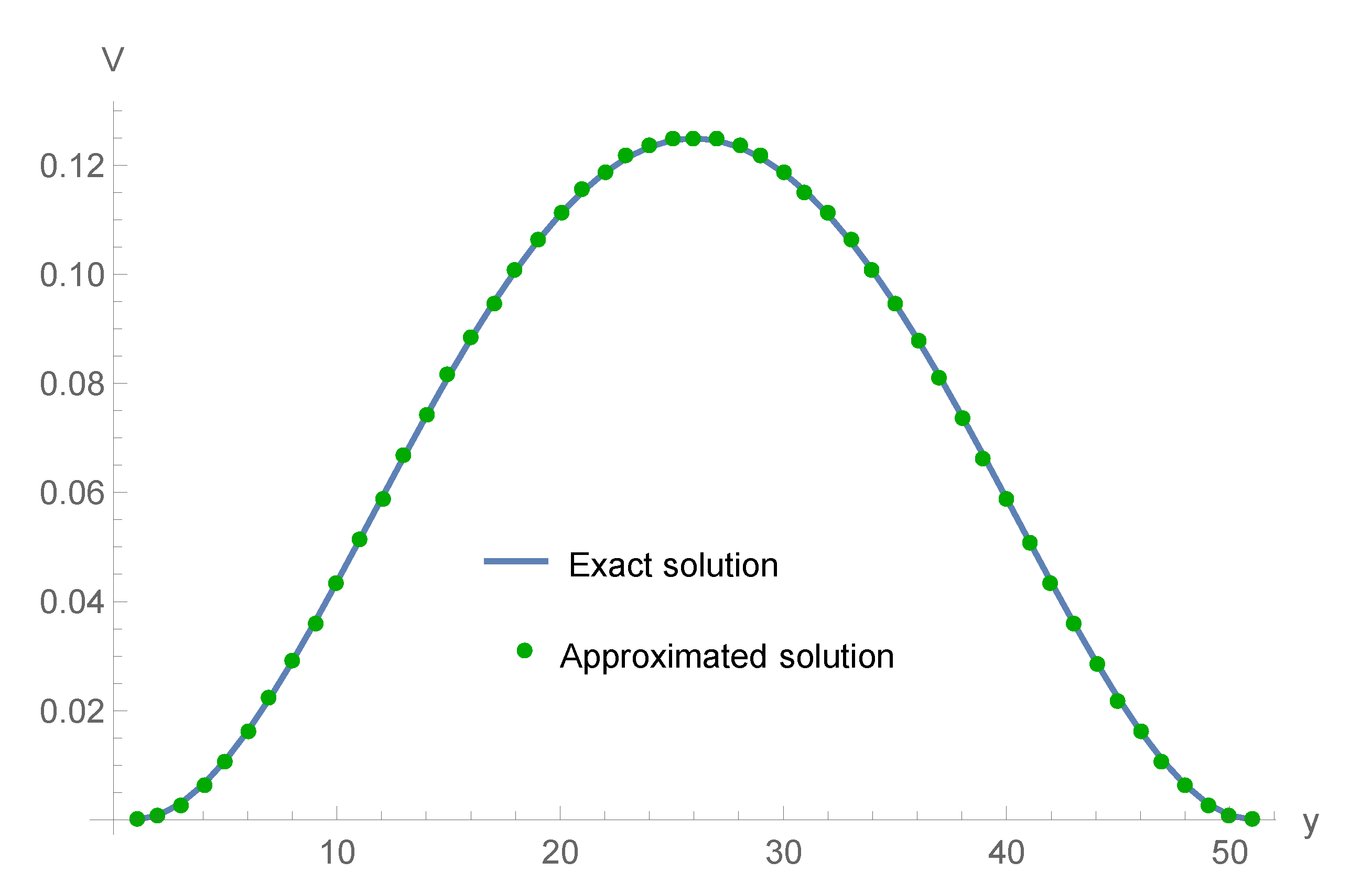
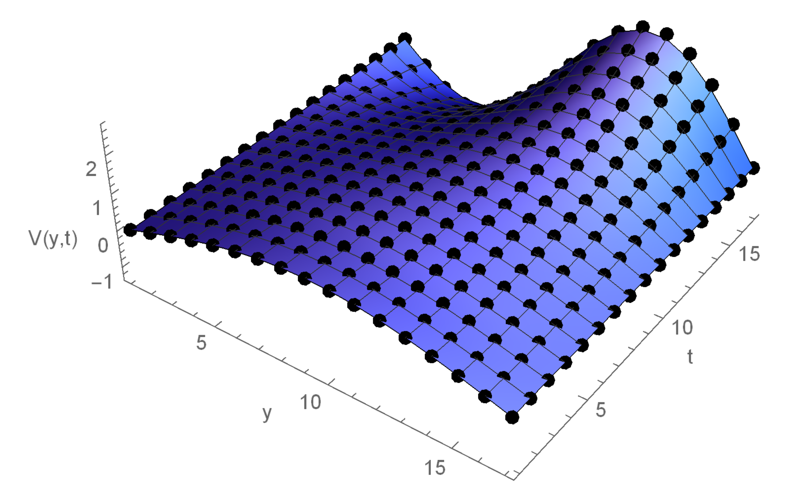
Table 1 shows the L , L 2 errors and order of the recommended technique for γ = 0.25 , 0.5 , α = 0.15 , h = 1 1024 at various τ . Table 2 presents the comparison of the L 2 errors with the results given by [16] and the order of convergence at different h. In Table 3, the absolute errors are demonstrated for the α = 0.15 and different γ at T = 1 . Figure 1 illustrates the 3D error plot of (1) for γ = 0.5 , α = 0.05 , when M = 16 and Q = 16 at T = 1 . Figure 2 shows the compatibility of exact and computed values for γ = 0.5 , α = 0.05 . In Figure 3, we present the approximated and exact graph of Example 1, for M = 50 , Q = 100 , γ = 0.5 , and α = 0.01 at T = 1 . Graphs show that the close relationship between the exact and calculated values.
Example 2.
Take the FPIDE with
V ( y , 0 ) = sin ( π y ) ,
and
G ( y , t ) = π π α t α 4 t 3 cos ( 2 π y ) sin ( π y ) + π 2 12 Γ ( 4 γ ) t 3 γ 2 π t 3 cos ( π y ) 48 π 2 γ ( α ) Γ ( α + 4 ) t 3 + α + ( 8 π t 6 cos ( 2 π y ) ) sin ( 2 π y ) .
The analytic solution is
V ( y , t ) = sin ( π y ) 2 t 3 sin ( 2 π y ) .
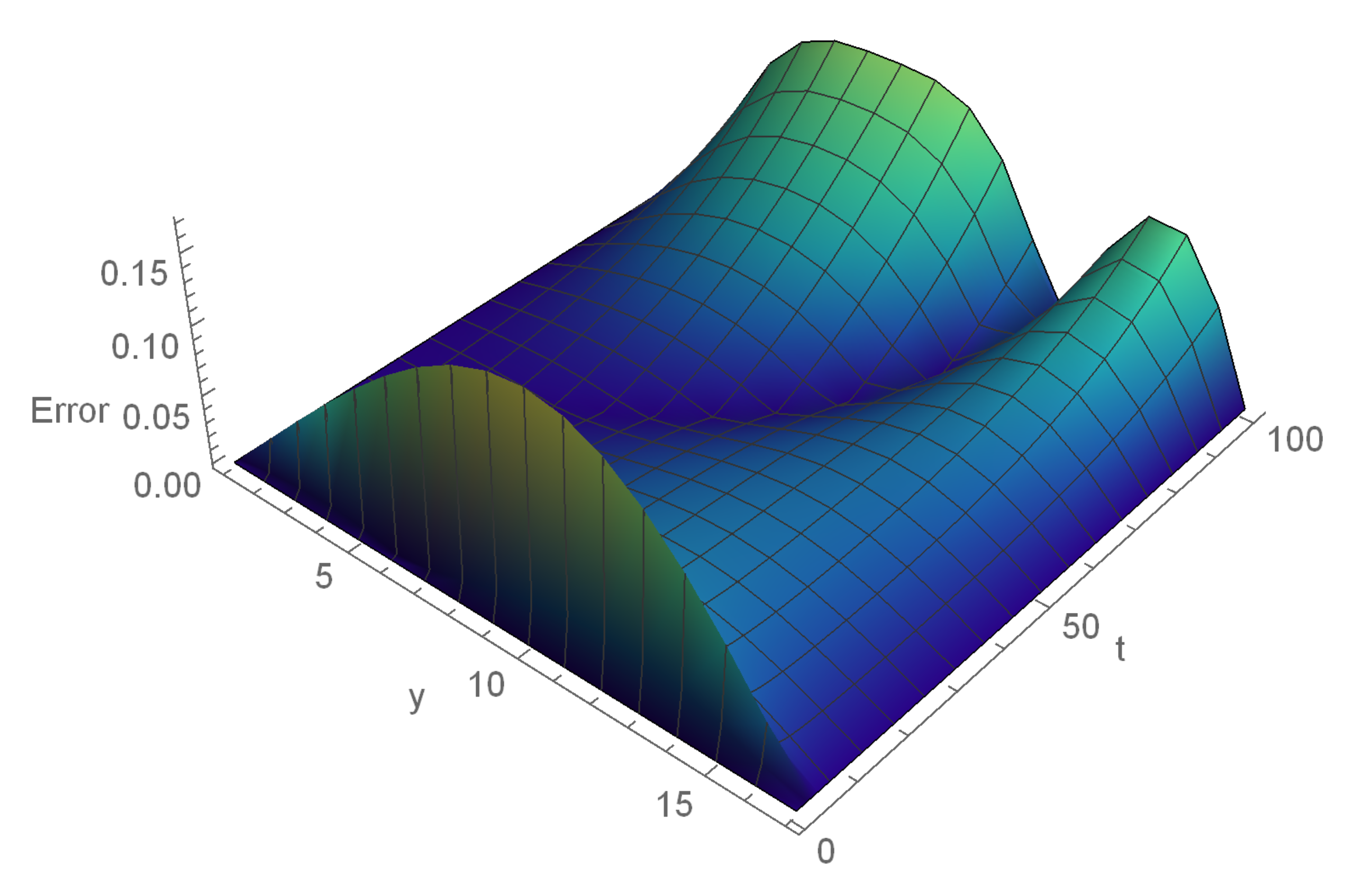
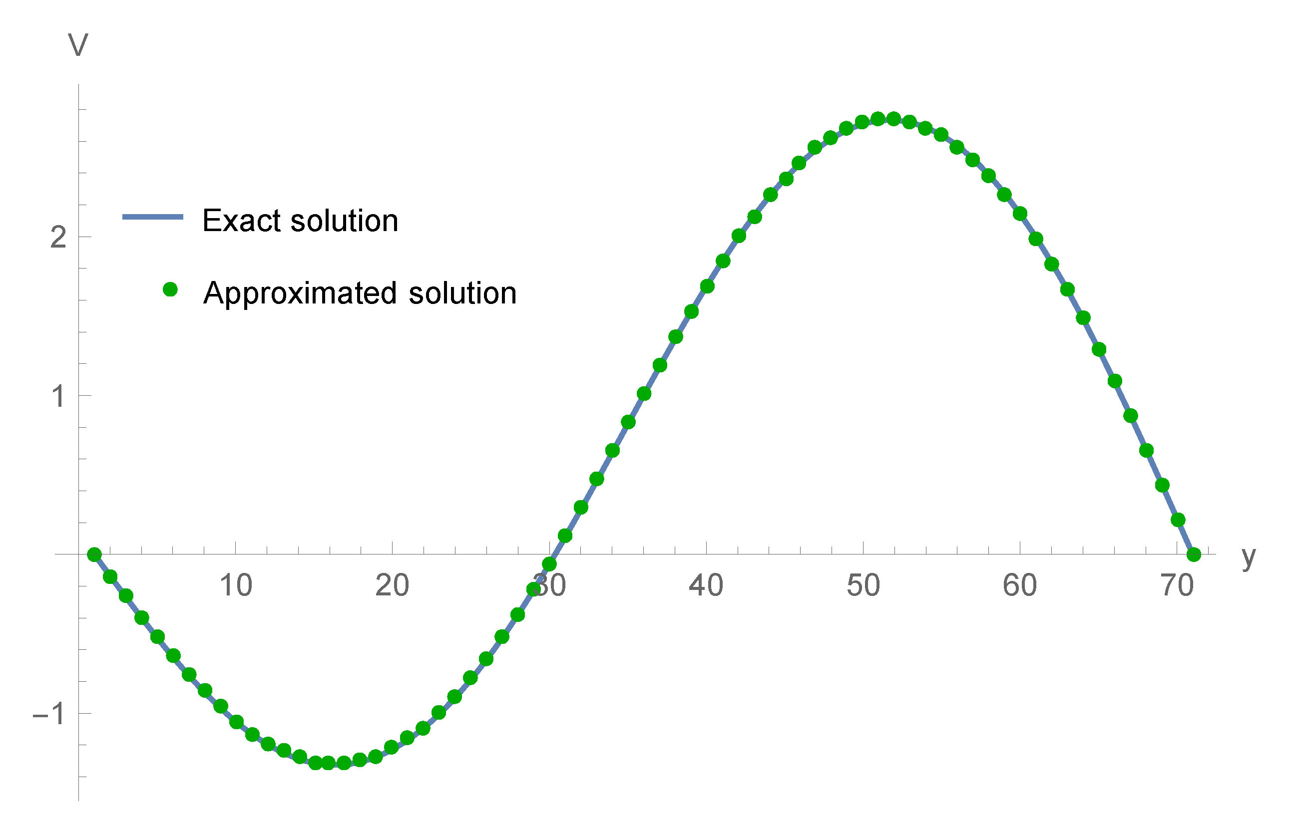
Table 4 demonstrates the L 2 and order in time side α = 0.15 , γ = 0.5 and various τ at T = 1 . In Table 5, the comparison of L 2 errors of 2 for α = 0.15 , γ = 0.5 , τ = 1 1000 at different h. In Table 6, we present the absolute errors for α = 0.05 and several values of γ at some knots, when h = 1 100 , τ = 1 100 , and T = 1 . Therefore, we achieve the convergence order in time direction is τ 2 γ , and space direction is 2. A comparison plot of computed and exact values has been displayed in Figure 4 for γ = 0.5 , α = 0.15 at T = 1 . Figure 5 depicts the errors of Example 2 for τ = 1 100 , α = 0.15 , γ = 0.5 for M = 16 and Q = 100 at T = 1 . The exact and calculated values are presented in Figure 6 for N = 70 , Q = 100 , γ = 0.5 , α = 0.01 .

6. Conclusions

In this manuscript, the ECBS collocation strategy is successfully described for the computed solutions of the nonlinear FPIDE with a weakly singular kernel. The CFD is approximated in terms of the finite difference technique. The discretized form of the CFD is applied to the time direction while the ECBS is utilized in the space dimension. In addition, the stability analysis and convergence analysis of the implemented algorithm is also presented to check the method is stable and convergent. The convergence order is demonstrated as ( τ 2 γ + h 2 ) , which is consistent with the theoretical results. Furthermore, The computational outcomes have been compared with the results given by [16] and some comparative findings demonstrate the effectiveness of the proposed collocation algorithm. The proposed technique can be implemented on the linear FPIDE model and the other linear and nonlinear second-order FPDEs. The suggested method can be extended for the higher-order hybrid and memory differential equations.

Author Contributions

Conceptualization, T.A., Z.A. and K.S.; investigation, T.A., Z.A., F.R., K.S. and P.K.; writing-original draft preparation, T.A., Z.A., F.R. and K.S.; writing-review and editing, T.A., Z.A., F.R., K.S. and P.K.; Funding acquisition, P.K. All authors have read and agreed to the published version of the manuscript.

Funding

“This research was funded by Thailand Science Research and Innovation (TSRI) Basic Research Fund: Fiscal year 2021 under project number 64A306000005” and “The APC was funded by the Center of Excellence in Theoretical and Computational Science (TaCS-CoE), KMUTT.”

Institutional Review Board Statement

Not applicable.

Informed Consent Statement

Not applicable.

Data Availability Statement

Not applicable.

Acknowledgments

The authors acknowledge the financial support provided by the Center of Excellence in Theoretical and Computational Science (TaCS-CoE), KMUTT.

Conflicts of Interest

The authors declare no conflict of interest.

References

  1. Atangana, A.; Secer, A. A Note on Fractional Order Derivatives and Table of Fractional Derivatives of Some Special Functions. Abstr. Appl. Anal. 2013, 2013, 279681. [Google Scholar] [CrossRef] [Green Version]
  2. Noeiaghdam, S.; Dreglea, A.; Iįk, H.; Suleman, M. A Comparative Study between Discrete Stochastic Arithmetic and Floating-Point Arithmetic to Validate the Results of Fractional Order Model of Malaria Infection. Mathematics 2021, 9, 1435. [Google Scholar] [CrossRef]
  3. Noeiaghdam, S.; Micula, S.; Nieto, J. A Novel Technique to Control the Accuracy of a Nonlinear Fractional Order Model of COVID-19: Application of the CESTAC Method and the CADNA Library. Mathematics 2021, 9, 1321. [Google Scholar] [CrossRef]
  4. Ali, Z.; Nia, S.N.; Rabiei, F.; Shah, K.; Tan, M.K. A Semianalytical Approach to the Solution of Time-Fractional Navier-Stokes Equation. Adv. Math. Phys. 2021, 2021, 13. [Google Scholar] [CrossRef]
  5. Mainardi, F. Fractional Calculus and Waves in Linear Viscoelasticity; Imperial College Press: London, UK, 2010. [Google Scholar]
  6. Zaslavsky, G.M. Hamiltonian Chaos and Fractional Dynamics; Oxford University Press: Oxford, UK, 2005. [Google Scholar]
  7. Podlubny, I. Fractional Differential Equations; Academic Press: San Diego, CA, USA, 1999. [Google Scholar]
  8. Kilbas, A.; Srivastava, H.; Trujillo, J. Theory and Applications of Fractional Differential Equations; Elsevier: Amsterdam, The Netherlands, 2006. [Google Scholar]
  9. Gurtin, M.E.; Pipkin, A.C. A general theory of heat conduction with finite wave speeds. Arch. Ration. Mech. Anal. 1968, 31, 113–126. [Google Scholar] [CrossRef]
  10. Pao, C.V.; Payne, L.; Amann, H. Bifurcation analysis of a nonlinear diffusion system in reactor dynamics. Appl. Anal. 2007, 9, 107–119. [Google Scholar] [CrossRef]
  11. Zadeh, K.S. An integro-partial differential equation for modeling biofluids flow in fractured biomaterials. J. Theor. Biol. 2011, 273, 72–79. [Google Scholar] [CrossRef]
  12. Hepperger, P. Hedging electricity swaptions using partial integro-differential equations. Stoch. Process. Their Appl. 2012, 122, 600–622. [Google Scholar] [CrossRef] [Green Version]
  13. Larsson, S.; Racheva, M.; Saedpanah, F. Discontinuous Galerkin method for an integro-differential equation modeling dynamic fractional order viscoelasticity. Comput. Methods Appl. Mech. Eng. 2015, 283, 196–209. [Google Scholar] [CrossRef] [Green Version]
  14. Mirzaee, F.; Alipour, S. A hybrid approach of nonlinear partial mixed integro-differential equations of fractional order. Iran. J. Sci. Technol. Trans. Sci. 2020, 44, 725–737. [Google Scholar] [CrossRef]
  15. Ng, F.S. Statistical mechanics of normal grain growth in one dimension: A partial integro-differential equation model. Acta Mater. 2016, 120, 453–462. [Google Scholar] [CrossRef] [Green Version]
  16. Guo, J.; Xu, D.; Qiu, W. A finite difference scheme for the nonlinear time-fractional partial integro-differential equation. Math. Methods Appl. Sci. 2020, 43, 1–21. [Google Scholar] [CrossRef]
  17. Hu, L.; Ren, Y.; Sakthivel, R. Existence and uniqueness of mild solutions for semilinear integro-differential equations of fractional order with nonlocal conditions. Semigroup Forum 2009, 79, 507–514. [Google Scholar] [CrossRef]
  18. Li, F.; Liang, J.; Xu, H.K. Existence of mild solutions for fractional integro-differential equations of Sobolev type with nonlocal conditions. J. Math. Anal. Appl. 2012, 391, 510–525. [Google Scholar] [CrossRef] [Green Version]
  19. Karthikeyan, K.; Trujillo, J.J. Existence and uniqueness results for fractional integrodifferential equations with boundary value conditions. Commun. Nonlinear Sci. Numer. Simul. 2012, 17, 4037–4043. [Google Scholar] [CrossRef]
  20. Chuong, N.M.; Ke, T.D.; Quan, N.N. Stability for a class of fractional partial integro-differential equations. J. Integral Equ. Appl. 2014, 26, 145–170. [Google Scholar] [CrossRef]
  21. Jaradat, H.; Awawdeh, F.; Rawashdeh, E.A. Analytic solution of fractional integro-differential equations. Ann. Univ. Craiova 2011, 38, 1–10. [Google Scholar]
  22. Hussain, A.K.; Rusli, N.; Fadhel, F.S.; Yahya, Z.R. Solution of one-dimensional fractional order partial integro-differential equations using variational iteration method. Aip Conf. Proc. 2016, 1775, 030096. [Google Scholar]
  23. Mittal, R.C.; Nigam, R. Solution of fractional integro-differential equations by Adomian decomposition method. Int. J. Appl. Math. Mech. 2008, 4, 87–94. [Google Scholar]
  24. Rawashdeh, E. Numerical solution of fractional integro-differential equations by collocation method. Appl. Math. Comput. 2006, 176, 1–6. [Google Scholar] [CrossRef]
  25. Eslahchi, M.R.; Dehghan, M.; Parvizi, M. Application of the collocation method for solving nonlinear fractional integro-differential equations. J. Comput. Appl. Math. 2014, 257, 105–128. [Google Scholar] [CrossRef]
  26. Zhao, J.; Xiao, J.; Ford, N.J. Collocation methods for fractional integro-differential equations with weakly singular kernels. Numer. Algor. 2014, 65, 723–743. [Google Scholar] [CrossRef]
  27. Arshed, S. B-Spline solution of fractional integro partial differential equation with a weakly singular kernel. Numer. Methods Partial. Differ. Equ. 2017, 33, 1565–1581. [Google Scholar] [CrossRef]
  28. Unhale, S.I.; Kendre, S.D. Numerical solution of nonlinear fractional integro-differential equation by Collocation method. Malaya J. Mat. 2018, 6, 73–79. [Google Scholar] [CrossRef] [Green Version]
  29. Avazzadeh, Z.; Heydari, M.H.; Cattani, C. Legendre wavelets for fractional partial integro-differential viscoelastic equations with weakly singular kernels. Eur. Phys. J. Plus 2019, 134, 368. [Google Scholar] [CrossRef]
  30. Dehestani, H.; Ordokhani, Y.; Razzaghi, M. Numerical solution of variable-order time fractional weakly singular partial integro-differential equations with error estimation. Math. Model. Anal. 2020, 25, 680–701. [Google Scholar] [CrossRef]
  31. Mohyud-Din, S.T.; Akram, T.; Abbas, M.; Ismail, A.I.; Ali, N.M. A fully implicit finite difference scheme based on extended cubic B-splines for time fractional advection-diffusion equation. Adv. Differ. Equ. 2018, 2018, 109. [Google Scholar] [CrossRef] [Green Version]
  32. Akram, T.; Abbas, M.; Ismail, A.I. An extended cubic B-spline collocation scheme for time fractional sub-diffusion equation. Aip Conf. Proc. 2019, 2184, 060017. [Google Scholar]
  33. Akram, T.; Abbas, M.; Ismail, A.I. Numerical solution of fractional cable equation via extended cubic B-spline. Aip Conf. Proc. 2019, 2138, 030004. [Google Scholar]
  34. Yaseen, M.; Abbas, M. An efficient computational technique based on cubic trigonometric B-splines for time fractional Burger’s equation. Int. J. Comput Math. 2019, 97, 725–738. [Google Scholar] [CrossRef] [Green Version]
  35. Jafari, H.; Khalique, M.; Ramezani, M.; Tajadodi, H. Numerical solution of fractional differential equations by using fractional B-spline. Cent. Eur. J. Phys. 2013, 11, 1372–1378. [Google Scholar] [CrossRef] [Green Version]
  36. Akram, T.; Abbas, M.; Ali, A.; Iqbal, A.; Baleanu, D. A Numerical Approach of a Time Fractional Reaction- Diffusion Model with a Non-Singular Kernel. Symmetry 2020, 12, 1653. [Google Scholar] [CrossRef]
  37. Akram, T.; Abbas, M.; Ismail, A.I.; Ali, N.M.; Baleanu, D. Extended cubic B-splines in the numerical solution of time fractional telegraph equation. Adv. Differ. Equ. 2019, 2019, 365. [Google Scholar] [CrossRef] [Green Version]
  38. Akram, T.; Abbas, M.; Iqbal, A.; Baleanu, D.; Asad, J. Novel Numerical Approach Based on Modified Extended Cubic B-Spline Functions for Solving Non-Linear Time-Fractional Telegraph Equation. Symmetry 2020, 12, 1154. [Google Scholar] [CrossRef]
  39. Han, L.X.; Liu, S.J. An extension of the cubic uniform B-spline curves. J. Comput Aided Des. Comput. Graph. 2003, 15, 576–578. [Google Scholar]
  40. Akram, T.; Abbas, M.; Riaz, M.B.; Ismail, A.I.; Ali, N.M. An efficient numerical technique for solving time fractional Burgers equation. Alex. Eng. J. 2020, 59, 2201–2220. [Google Scholar] [CrossRef]
  41. Rubin, S.G.; Graves, R.A. A Cubic Spline Approximation for Problems in Fluid Mechanics; NASA Technical Report; U.S. National Aeronautics and Space Administration: Washington, DC, USA, 1975; Available online: https://books.google.com.my/books?id=tzbGKg7dV-IC (accessed on 2 August 2021).
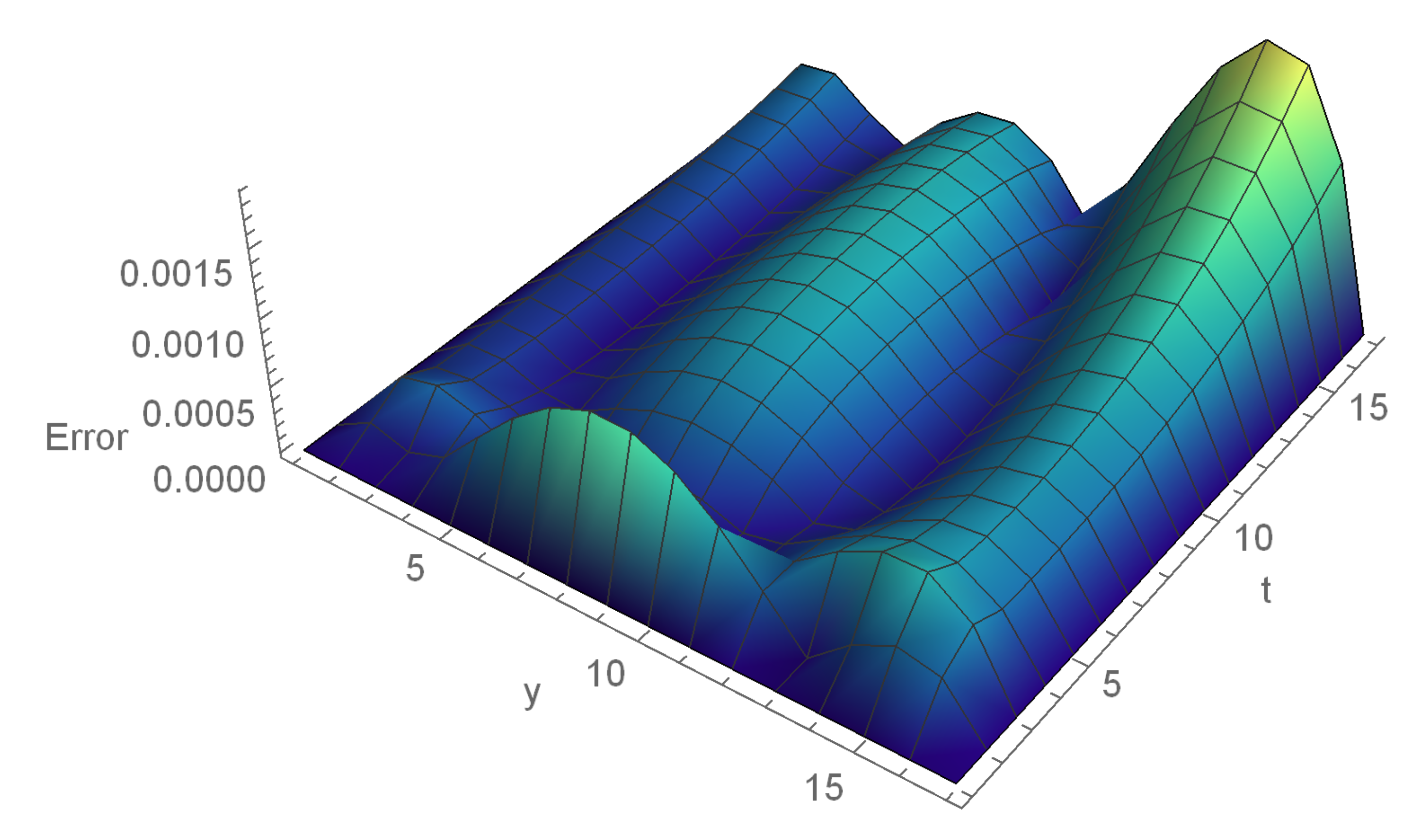
Figure 1. Error graph of Example 1 at γ = 0.5 and α = 0.05 .
Fractalfract 05 00085 g001
Figure 2. Comparison of the exact (dots) and the computed values (solid lines) of Example 1 at γ = 0.5 and α = 0.05 .
Fractalfract 05 00085 g002
Figure 3. Comparison of the exact and the computed values at γ = 0.5 and α = 0.01 .
Fractalfract 05 00085 g003
Figure 4. A Comparison plot (dots show the exact solution while the solid lines illustrate approximated solution) of Example 2 at γ = 0.5 and α = 0.15 .
Fractalfract 05 00085 g004
Figure 5. Error graph of Example 2 for α = 0.15 , N = 16 at T = 1 .
Fractalfract 05 00085 g005
Figure 6. Comparison of the exact and the computed values of Example 2 at γ = 0.5 and α = 0.01 .
Fractalfract 05 00085 g006
Table 1. The L , L 2 errors of Example 1 for α = 0.15 , h = 1 1024 , at T = 1 .
γ τ ECBS
L 2 [16] L 2 L Order
0.251/40.0003389280.0001023310.005061940
0.251/80.0000953870.0000319340.0015075301.74750
0.251/160.0000260070.0000085420.0004456851.75809
0.251/320.0000067880.0000018820.0001336311.73777
0.51/40.0003368090.0001021830.00505510
0.51/80.0000506280.0000319760.001510141.74750
0.51/160.0000256300.0000081780.000455651.72618
0.51/320.0000067840.0000019550.000134911.75595
Table 2. The L , L 2 errors of Example 1 for α = 0.15 , τ = 1 1000 , at T = 1 .
γ h ECBS
L 2 [16] L 2 L Order
0.51/40.02233890.018223700.0549348
0.51/80.00559910.003451800.01364262.00960
0.51/160.00140020.000783400.00331252.04213
0.51/320.00035010.000025050.000801642.04690
Table 3. Absolute errors Example 1 for α = 0.15 , at various knots.
y γ = 0.25 γ = 0.50 γ = 0.75 γ = 0.95
0.10.00022780.00023930.00026110.0000426
0.20.00187830.00190050.00194300.0011812
0.30.00357170.00360340.00366390.0023206
0.40.00428660.00432570.00439970.0026410
0.50.00347570.00351960.00360080.0017125
0.60.00119750.00124210.00132300.0003752
0.70.00179310.00175250.00168050.0029206
0.80.00407880.00404740.00399300.0046428
0.90.00389640.00387920.00384970.0039922
Table 4. The L 2 errors of Example 2 for α = 0.15 , h = 1 1024 , at T = 1 .
γ τ L 2 [16] L 2 Order
0.51/40.01774090.0130166
0.51/80.00512290.00505671.489999
0.51/160.00142720.00112561.495493
0.51/320.00038660.00030481.497291
Table 5. The L 2 errors of Example 2 for α = 0.15 , τ = 1 1000 , at T = 1 .
γ h L 2 [16] L 2 Order
0.51/40.32957130.2219332
0.51/80.07508750.04564381.489999
0.51/160.01834640.00587521.495493
0.51/320.00456050.00068861.497291
Table 6. Absolute errors of Example 2 for α = 0.05 , at various connections.
y γ = 0.25 γ = 0.50 γ = 0.75 γ = 0.95
0.10.02374470.02165250.02244320.0224217
0.20.03643580.03325490.03444750.0344188
0.30.03906150.03643040.03736760.0373676
0.40.03918210.03872130.03880310.0388078
0.50.03632140.03891810.03778290.0378141
0.60.02142060.02677980.02455920.0246163
0.70.00627880.00043000.02566910.0022242
0.80.02929140.02322630.00399300.0255941
0.90.02700440.02342840.02486000.0248123
Publisher’s Note: MDPI stays neutral with regard to jurisdictional claims in published maps and institutional affiliations.