Reduced Multiplicative (BURA-MR) and Additive (BURA-AR) Best Uniform Rational Approximation Methods and Algorithms for Fractional Elliptic Equations

Abstract

Numerical methods for spectral space-fractional elliptic equations are studied. The boundary value problem is defined in a bounded domain of general geometry, $\Omega \subset {\mathbb{R}}^d$, $d\in \{1,2,3\}$. Assuming that the finite difference method (FDM) or the finite element method (FEM) is applied for discretization in space, the approximate solution is described by the system of linear algebraic equations ${\mathbb{A}}^{\alpha }\mathbf{u}=\mathbf{f}$, $\alpha \in (0,1)$. Although matrix $\mathbb{A}\in {\mathbb{R}}^{N\times N}$ is sparse, symmetric and positive definite (SPD), matrix ${\mathbb{A}}^{\alpha }$ is dense. The recent achievements in the field are determined by methods that reduce the original non-local problem to solving k auxiliary linear systems with sparse SPD matrices that can be expressed as positive diagonal perturbations of $\mathbb{A}$. The present study is in the spirit of the BURA method, based on the best uniform rational approximation $r_{\alpha ,k}\left(t\right)$ of degree k of $t^{\alpha }$ in the interval $[0,1]$. The introduced additive BURA-AR and multiplicative BURA-MR methods follow the observation that the matrices of part of the auxiliary systems possess very different properties. As a result, solution methods with substantially improved computational complexity are developed. In this paper, we present new theoretical characterizations of the BURA parameters, which gives a theoretical justification for the new methods. The theoretical estimates are supported by a set of representative numerical tests. The new theoretical and experimental results raise the question of whether the almost optimal estimate of the computational complexity of the BURA method in the form $O\left(N{log}^{2}N\right)$ can be improved.

1. Introduction

The basic assumption about the fractional diffusion phenomenon is that the Brownian motion hypothesis is violated. In the case of isotropic homogeneous media, such processes are described by the fractional Laplacian. A natural and easy-to-comprehend presentation of fractional Laplacian in the whole space ${\mathbb{R}}^d$, $d=1,2,3$ can be derived through the Fourier transform. Serious (not only computational) challenges appear when the equation is posed in a bounded domain $\Omega$, equipped with the correct boundary conditions, and the related boundary value problem is considered. There exist at least two different and not equivalent definitions of fractional Laplacian [1,2]. They follow the spectral and the Riesz formulations, respectively. Some recent comparison results between those two approaches are presented in [3], where the difference of the asymptotes of boundary layers is analyzed in detail.

In this paper, we consider the spectral fractional elliptic equation with power $\alpha \in (0,1)$, which is in the form

$${\mathcal{A}}^{\alpha }u\left(x\right)=f\left(x\right),$$

(1)

where $\mathcal{A}$ is a self-adjoint elliptic operator in $\Omega$, satisfying homogeneous Dirichlet boundary conditions. The non-local operator ${\mathcal{A}}^{\alpha }$ is defined via the spectral decomposition of $\mathcal{A}$, namely

$${\mathcal{A}}^{\alpha }u=\sum _{j=1}^{\infty }{\lambda }_j^{\alpha }(u,{\psi }_j){\psi }_j,$$

(2)

where ${\lambda }_j>0$ are the eigenvalues, respectively, ${\psi }_j$ are the corresponding normalized eigenfunctions of $\mathcal{A}$, and  $(...)$ is the $L^2$ inner product.

Let ${\omega }_h$ be a uniform rectangular mesh, and the finite difference method (FDM) using a standard $(2d+1)$-stencil is applied for approximating the operator $\mathcal{A}$. Then, the FDM discretization of (1) leads to a system of linear algebraic equations with respect to the mesh functions $\mathbf{u}$ and $\mathbf{f}$ in the form

$${\mathbb{A}}^{\alpha }\mathbf{u}=\mathbf{f}.$$

(3)

Here, $\mathbb{A}\in {\mathbb{R}}^{N\times N}$ is a sparse, symmetric and positive definite (SPD) matrix, and 

$${\mathbb{A}}^{\alpha }\mathbf{u}=\sum _{j=1}^N{\lambda }_{j,h}^{\alpha }(\mathbf{u},{\mathsf{\Psi }}_{j,h}){\mathsf{\Psi }}_{j,h}.$$

(4)

As in the continuous case, ${\left\{{\lambda }_{j,h}\right\}}_{j=1}^N$ is the spectrum of $\mathbb{A}$, and the eigenvectors ${\mathsf{\Psi }}_{j,h}$ are normalized with respect to the Euclidean dot product $(...)$. Similar construction is applicable when the finite element method (FEM), using a quasi uniform triangulation ${\mathcal{T}}_h$, is applied. In this case, $\mathbb{A}={\mathbb{M}}^{-1}\mathbb{K}$, where $\mathbb{K}$ and $\mathbb{M}$ are the FEM stiffness and mass matrices, respectively, and $\mathbb{A}$ is SPD with respect to the scalar product generated by the mass matrix. In what follows, we assume that linear finite elements are used.

The recent achievements in the numerical solution of spectral fractional elliptic equations are determined by the class of methods that are applicable to multidimensional domains $\Omega$ of general geometry; see [4,5], the references therein, as well as the most recent paper [6]. Although there are several rather different approaches there, all the obtained algorithms reduce the original non-local problem to solving k auxiliary linear systems with sparse SPD matrices that can be expressed as some diagonal perturbations of $\mathbb{A}$ in the form $\mathbb{A}-d_i\mathbb{I}$, $d_i<0$, $i=1,\dots k$. Thus, all these methods can be interpreted as certain rational approximations of degree k [4,7], i.e., ${\mathbb{A}}^{-\alpha }\approx {\tilde{r}}_{\alpha ,k}\left(\mathbb{A}\right)$. In this context, the advantages of the BURA method [4,5,8,9] follow directly by its definition, as being the best uniform rational approximation $r_{\alpha ,k}$ of degree k for $t^{\alpha }$ in $[0,1]$.

Introducing the BURA method [9], the modified Remez algorithm was applied to derive $r_{\alpha ,k}$. However, it faces serious difficulties regarding the computational stability for larger k and smaller $\alpha$. The results obtained in the last few years largely overcome this problem. For example, in [7], the Chebfun implementation of the adaptive Antoulas-Anderson (AAA) algorithm is applied, where the representation of the rational approximant in barycentric form and greedy selection of the support points is used to approximate $z^{-\alpha }$ for $z\in [{\lambda }_{1,h},{\lambda }_{N,h}]$. Further progress in this direction has been made in [10] (see [11] for the related software implementation). The algorithm (BRASIL) is based on the introduced barycentric rational interpolation. The new algorithms and software tools for stable computation of best uniform rational approximations for larger degrees k provide promising opportunities with respect to further expansions of the application of the BURA technology and its better understanding and interpretation.

The next four publications [12,13,14,15] are in the spirit of further development of methods based on best uniform rational approximations.

Solving time-fractional differential equations is considered in [13], where the spectrum of the fractional Laplace kernel is approximated with a rational function, applying the AAA algorithm. Stability and convergence properties of the proposed numerical scheme are studied. Moreover, the developed algorithm is efficiently applied to a time-fractional Cahn–Hilliard problem.

A class of Reduced Basis Methods (RBM) is studied in [12]. Based on the developed theory, the equivalence between RBM and Rational Krylov Methods (RKM) is analyzed in [14]. Then a unified RKM framework for the spectral fractional in space and fractional in time problems is proposed in [15].

The methods discussed above have a strong impact on the development of efficient solution methods for fractional diffusion problems beyond the scalar elliptic case (see, e.g., [4]). Such results are presented in the more recent papers [16,17], where nonlinear and time-dependent fractional diffusion-in-space problems are considered, respectively. In this spirit, the results are also presented in [18], where a tensor numerical method for optimal control problems constrained by a fractional elliptic operator is developed.

In many studies, the needed degree k for obtaining the targeted accuracy of ${\tilde{r}}_{\alpha ,k}\left(\mathbb{A}\right)$ is considered as a measure for the computational efficiency of the method. This holds true under the assumption that the complexity of the method is $O\left(kN\right)$. In the case of a large scale unstructured matrix $\mathbb{A}$, this means that some iterative method of optimal complexity $O\left(N\right)$ is used for solving the auxiliary systems. Obviously, these auxiliary systems possess very different properties. More recently [19], it was found that for larger k, part of the coefficients $-d_i$ can be extremely large. This observation motivates the proposed reduced sum modification of the additive BURA method, called BURA-AR.

In this paper, we present new theoretical characterizations of the BURA parameters, which gives theoretical justification of the BURA-AR method and the newly proposed reduced product multiplicative BURA-MR method. In this way, a significant improvement in computational complexity is achieved. The presented numerical results can be used as direct practical receipts for optimizing the computational complexity, depending on the fractional power $\alpha$. The new theoretical and experimental results raise the question of whether the current state-of-the-art almost-optimal estimate of the computational complexity of the BURA method in the form $O\left(N{(logN)}^2\right)$ can be improved.

The rest of the paper is organized as follows. Some basic definitions, error estimates, and additive and multiplicative representations of the BURA algorithm are given in Section 2. BURA’s stabilized calculations for larger k are discussed in the next section. It includes a comparative analysis of the theoretical error estimates and the accuracy of BURA, computed using the BRASIL software. Important theoretical results are presented in Section 4. The obtained characterization of the BURA parameters includes interlacing inequalities and asymptotic cluster analysis. The BURA-AR and BURA-MR methods are introduced in the next section. It is shown how to optimize the new parameter l in order to obtain the best computational complexity for a given target accuracy and given a priori estimates of the extreme eigenvalues ${\lambda }_{1,h}$ and ${\lambda }_{N,h}$. The numerical results presented in Section 6 confirm the efficiency of the developed computational technology. The considered large-scale 3D numerical tests illustrate the influence of the fractional power $\alpha$ depending on the smoothness of the right-hand side $f\left(x\right)$. Brief concluding remarks are given at the end.

2. The BURA Method

The abbreviation BURA stands for best uniform rational approximation. Let us consider the min-max problem: find $r_{\alpha ,k}\in \mathcal{R}(k,k)$ such that

$$\underset{t\in [0,1]}{max}|t^{\alpha }-r_{\alpha ,k}\left(t\right)|=\underset{r_k\left(t\right)\in \mathcal{R}(k,k)}{min}\underset{t\in [0,1]}{max}|t^{\alpha }-r_k\left(t\right)|,\alpha \in (0,1),$$

where $r_k\left(t\right)=P_k\left(t\right)/Q_k\left(t\right)$, $P_k$ and $Q_k$ are polynomials of degree k. Then the error $E_{\alpha ,k}$ of the k-BURA element $r_{\alpha ,k}$ is defined as

$$E_{\alpha ,k}:=\underset{t\in [0,1]}{max}|t^{\alpha }-r_{\alpha ,k}\left(t\right)|.$$

(5)

A sharp estimate of $E_{\alpha ,k}$ is derived in [20]:

$$E_{\alpha ,k}=4^{\alpha +1}sin\left(\alpha \pi \right)e^{-2\pi \sqrt{\alpha k}}.$$

(6)

Following [5] we introduce the approximation of ${\mathbb{A}}^{-\alpha }$ in the form

$${\mathbb{A}}^{-\alpha }\approx {\lambda }_{1,h}^{-\alpha }{r}_{\alpha ,k}\left({\lambda }_{1,h}{\mathbb{A}}^{-1}\right),$$

and then

$${\mathbf{u}}_k={\lambda }_{1,h}^{-\alpha }{r}_{\alpha ,k}\left({\lambda }_{1,h}{\mathbb{A}}^{-1}\right)\mathbf{f},$$

(7)

where ${\mathbf{u}}_k$ is the BURA numerical solution of the linear algebraic system (3). In other words, ${\mathbf{u}}_k$ is the BURA approximation of the solution $u\left(x\right)$ of the fractional elliptic Equation (1).

The following error estimate of the BURA method holds true.

Property 1

(see [5] p. 19). Let $\Omega \subset {\mathbb{R}}^2$, and let the lumped mass linear finite elements for discretization in space be used. Then

$$\parallel {\mathcal{A}}^{-\alpha }f-u_{h,k}{\parallel }_{L^2}\le C(h^{2\alpha }+h^{1+\gamma }){\parallel f\parallel }_{H^{1+\gamma }(\Omega )}+{\lambda }_{1,h}^{-\alpha }{E}_{\alpha ,k}{\parallel f\parallel }_{L^2},$$

(8)

and therefore

$$\parallel {\mathcal{A}}^{-\alpha }f-u_{h,k}{\parallel }_{L^2}\le C(h^{2\alpha }+h^{1+\gamma }+e^{-2\pi \sqrt{k\alpha }}){\parallel f\parallel }_{H^{1+\gamma }(\Omega )},$$

(9)

with $\gamma >0$, and C independent of h and k. Here $u_{h,k}$ is the FEM function corresponding to the BURA approximation ${\mathbf{u}}_k$.

Remark 1.

The equivalence of the lumped linear FEM and FDM discretizations on uniform rectangle meshes allows obtaining analogues of the error estimates (9)–(11) for the case of the finite difference method.

As noted in [5], for $\Omega \subset {\mathbb{R}}^d$, $d=1,3$, the estimates (8) and (9) remain valid provided that $1+\gamma$ is replaced by $d/2+\gamma$. In this way, in the more interesting three-dimensional case, one can obtain the error bounds

$$\parallel {\mathcal{A}}^{-\alpha }f-u_{h,k}{\parallel }_{L^2}\le C(h^{2\alpha }+h^{3/2+\gamma }){\parallel f\parallel }_{H^{3/2+\gamma }(\Omega )}+{\lambda }_{1,h}^{-\alpha }{E}_{\alpha ,k}{\parallel f\parallel }_{L^2},$$

(10)

that is

$$\parallel {\mathcal{A}}^{-\alpha }f-u_{h,k}{\parallel }_{L^2}\le C(h^{2\alpha }+h^{3/2+\gamma }+e^{-2\pi \sqrt{k\alpha }}){\parallel f\parallel }_{H^{3/2+\gamma }(\Omega )},$$

(11)

where $\Omega \subset {\mathbb{R}}^3$.

An additive or multiplicative representation of the rational function $r_{\alpha ,k}(1/z)$ can be used for implementation of the BURA method. Till  now, the first one is preferred, but in this paper we will analyze both of them independently. The additive representation relies on the partial fraction decomposition of $r_{\alpha ,k}$, while the multiplicative one deals with the factorization of $r_{\alpha ,k}$:

$${\tilde{r}}_{\alpha ,k}\left(z\right):=r_{\alpha ,k}(1/z)={\tilde{c}}_0+\sum _{i=1}^k\frac{{\tilde{c}}_i}{z-{\tilde{d}}_i}={\tilde{c}}_0\prod _{i=1}^k\frac{z-{\tilde{\xi }}_i}{z-{\tilde{d}}_i},$$

(12)

where ${\tilde{c}}_i>0$ and ${\tilde{d}}_i,{\tilde{\xi }}_i<0$. In these ways, the BURA method reads as

$$\begin{array}{cc}\hfill {\mathbf{u}}_k& ={\lambda }_{1,h}^{-\alpha }\left[{\tilde{c}}_0\mathbb{I}+\sum _{i=1}^k\left({\lambda }_{1,h}{\tilde{c}}_i\right){(\mathbb{A}-{\lambda }_{1,h}{\tilde{d}}_i\mathbb{I})}^{-1}\right]\mathbf{f},\hfill \\ \hfill {\mathbf{u}}_k& ={\lambda }_{1,h}^{-\alpha }{\tilde{c}}_0\prod _{i=1}^k\left[(\mathbb{A}-{\lambda }_{1,h}{\tilde{\xi }}_i\mathbb{I}){(\mathbb{A}-{\lambda }_{1,h}{\tilde{d}}_i\mathbb{I})}^{-1}\right]\mathbf{f}.\hfill \end{array}$$

(13)

Thus, the BURA method for numerical solution of the fractional differential Equation (1) requires the solving of k auxiliary linear systems with sparse SPD matrices, which are positive diagonal shifts of the FEM/FDM matrix $\mathbb{A}$.

The unified view of the methods for solving Equation (1) as a rational approximation [4,7] leads to a general understanding of the degree k as a measure for computational efficiency. Thus, for the computational complexity of the BURA method, we accept that the following asymptotic estimate holds true:

$${\mathcal{N}}_{\alpha ,k}^{BURA}=O\left(kN\right).$$

(14)

This is valid if a method with optimal computational complexity is used to solve the auxiliary linear systems that appear in (13). In the multidimensional case, this means that such an iterative solver is applied. In  our numerical tests, we used the BoomerAMG implementation from HYPRE [21] of the algebraic multigrid preconditioner in the PCG framework.

The further analysis is based on the error estimates (9)–(11). From there, choosing properly the mesh parameters h and the BURA order k, the contributions of the discretization and the BURA approximation to the total error are balanced. In this way, the following almost optimal computational complexity of the BURA algorithms is obtained

$${\mathcal{N}}_{\alpha ,k}^{BURA}=O\left(N{(logN)}^2\right).$$

(15)

Improving the computational efficiency of the BURA method is the central focus of this paper. The analysis of the BURA parameters, and in particular of the coefficients ${\tilde{d}}_i$, determining the diagonal shifts of $\mathbb{A}$ in (13), is behind the developed approach.

3. BURA: Stabilized Computations for Large k

In [4], a modified Remez algorithm (see [22]) was used for the computation of the BURA element of a degree up to ten. This algorithm is very time consuming and because of the difficulties related to the computational stability for large k’s in [19], we used the Best Rational Approximation by Successive Interval Length (BRASIL) [11] to get the BURA of degree 85. Here, we computed the error of the rational approximation of the function $t^{\alpha }$ in the interval $[0,1]$ obtained using the BRASIL software version 1.2.1. We used the following options in baryrat.brasil:

tol $=2^{-52}$	convergence criterion tolerance;
npi $=-30$	30 iterations of golden section search per interval;
maxiter =10,000	the maximum number of iterations.

The BRASIL algorithm is based on a barycentric representation of the rational approximation of the form

$$r_{\alpha ,k}^{\left(BR\right)}\left(t\right)=\frac{{\sum }_{i=0}^k\frac{w_i}{t-t_i}{f}_i}{{\sum }_{i=0}^k\frac{w_i}{t-t_i}}.$$

In order to obtain the coefficients of the simple additive representation (12), we first find the roots ${\left\{{\xi }_i\right\}}_{i=1}^k$ and the poles ${\left\{d_i\right\}}_{i=1}^k$ of the above barycentric representation. This is already implemented in the baryrat package by solving a corresponding eigenvalue problem using arithmetical precision of 100 decimal places (provided by the mpmath Python package). Since we are interested in ${\tilde{r}}_{\alpha ,k}\left(z\right)=r_{\alpha ,k}\left(z^{-1}\right)$ our roots and poles will be ${\{{\tilde{\xi }}_i={\xi }_i^{-1}\}}_{i=1}^k$ and ${\{{\tilde{d}}_i=d_i^{-1}\}}_{i=1}^k$, respectively. Therefore, we can straightforwardly compute ${\tilde{d}}_i$. To find the values of the ${\tilde{c}}_i$ coefficients in (12), we then solve the following linear system

$$\left[\begin{array}{cccc}1& {(1-{\tilde{d}}_1)}^{-1}& \cdots & {(1-{\tilde{d}}_k)}^{-1}\\ 1& {({\tilde{\xi }}_1-{\tilde{d}}_1)}^{-1}& \cdots & {({\tilde{\xi }}_1-{\tilde{d}}_k)}^{-1}\\ ⋮& ⋮& \ddots & ⋮\\ 1& {({\tilde{\xi }}_k-{\tilde{d}}_1)}^{-1}& \cdots & {({\tilde{\xi }}_k-{\tilde{d}}_k)}^{-1}\end{array}\right]\left[\begin{array}{c}{\tilde{c}}_0\\ {\tilde{c}}_1\\ ⋮\\ {\tilde{c}}_k\end{array}\right]=\left[\begin{array}{c}{r}_{\alpha ,k}^{\left(BR\right)}\left(1\right)\\ 0\\ ⋮\\ 0\end{array}\right].$$

For the solution of the above linear system, we have also used the mpmath package with a precision of 100 decimal places.

Let us also note that here we are using a modified convergence criterion for the BRASIL algorithm to ensure that the algorithm converges for large values of k without tinkering with the tolerance. The BRASIL algorithm first computes the errors

$${\delta }_i=\underset{t\in (t_{i-1},t_i)}{max}|t^{\alpha }-r_{\alpha ,k}^{\left(BR\right)}\left(t\right)|$$

for each interval between the interpolation points. Convergence is then decided, based on comparing the deviation of the errors in each interval to the tolerance

$$\frac{{max}_i{\delta }_i}{{min}_i{\delta }_i}-1<\epsilon .$$

The issue with the above is that $\epsilon$ has to be changed for different values of k. When the errors become very small, the arithmetical error in computing the deviation becomes significant and the algorithm stops converging for small values of $\epsilon$. Instead of only looking at the deviation, we are checking the product of the maximum error and the deviation

$$\underset{i}{max}{\delta }_i\left(\frac{{max}_i{\delta }_i}{{min}_i{\delta }_i}-1\right)\le 2^{-52}.$$

The idea is to automatically get as close to the BURA as double-precision floating point arithmetics would allow.

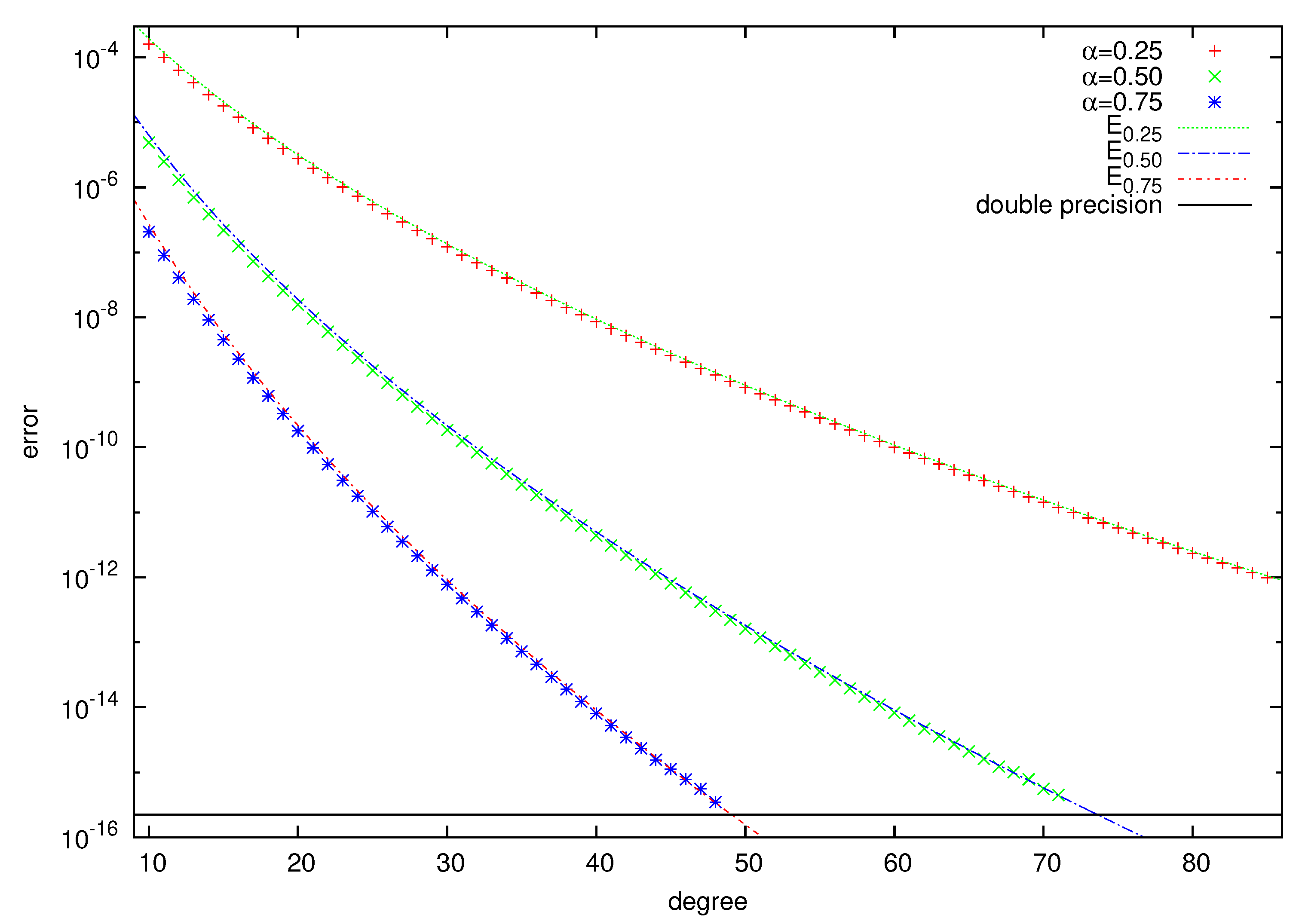
The errors for the values of $\alpha =\frac{1}{4},\frac{1}{2},\frac{3}{4}$ are presented in Figure 1. We compare these errors with the theoretical estimate (6) of the BURA error from [20]. It is easy to see that the computed errors are very close to the theoretical estimate when the estimate is greater than the double-precision accuracy. The comparison shows that the theoretical estimate of the error is sharp.

4. Theoretical Characterizations of the Parameters of BURA

4.1. In the Unit Interval $t\in [0,1]$

The multiplicative and the additive representations of $r_{\alpha ,k}\left(t\right)$ are the following:

$$r_{\alpha ,k}\left(t\right)=c_0\prod _{i=1}^k\frac{t-{\xi }_i}{t-d_i}=c_0+\sum _{i=1}^k\frac{c_i}{t-d_i}.$$

(16)

Note that due to ${lim}_{t\to \infty }{r}_{\alpha ,k}\left(t\right)=c_0$, the coefficients $c_0$ in both formulas above coincide.

Theorem 1

(see [20,23]). For arbitrary $\alpha \in (0,1)$ and $k\in \mathbb{N}$ the following holds true:

(a)

The zeros and the poles of $r_{\alpha ,k}$ are real, negative, and interlacing:

$$0>{\xi }_1>d_1>{\xi }_2>d_2>\cdots >{\xi }_k>d_k>-\infty$$

(17)

(b)

The error function ${\epsilon }_{\alpha ,k}\left(t\right):=t^{\alpha }-r_{\alpha ,k}\left(t\right)$ has exactly $2k+2$ extreme points ${\eta }_1,{\eta }_2,\cdots ,{\eta }_{2k+2}$ on $[0,1]$, such that

$$0={\eta }_1<{\eta }_2<\cdots <{\eta }_{2k+2}=1,{\epsilon }_{\alpha ,k}\left({\eta }_i\right)={(-1)}^i{E}_{\alpha ,k},i=1,\cdots ,2k+2.$$

(18)

(c)

The number of poles and zeros of $r_{\alpha ,k}$ on any given closed subinterval $[a,b]\subseteq {\mathbb{R}}_{<0}$ grows like $\sqrt{k}$ as $k\to \infty$, i.e., for all $-\infty \le a\le b<0$

$$\underset{k\to \infty }{lim}\frac{1}{\sqrt{k}}card\{{\xi }_i\in [a,b]\}=\underset{k\to \infty }{lim}\frac{1}{\sqrt{k}}card\{d_i\in [a,b]\}=\frac{\sqrt{\alpha }}{\pi }{\int }_{\left|b\right|}^{\left|a\right|}\frac{dt}{t\sqrt{1+t}}.$$

(19)

(d)

The number of extreme points of ${\epsilon }_{\alpha ,k}$ on any given closed subinterval $[a,b]\subseteq (0,1]$ grows like $\sqrt{k}$ as $k\to \infty$, i.e., for all $0<a\le b\le 1$

$$\underset{k\to \infty }{lim}\frac{1}{\sqrt{k}}card\{{\eta }_i\in [a,b]\}=\frac{2\sqrt{\alpha }}{\pi }{\int }_a^b\frac{dt}{t\sqrt{1-t}}.$$

(20)

Lemma 1.

Let $\alpha \in (0,1)$. As $k\to \infty$, almost all poles and zeros of $r_{\alpha ,k}$, as well as extreme points of ${\epsilon }_{\alpha ,k}$ tend to the origin.

Proof. 

Fix $m\in \mathbb{N}$. We will show that for every $\epsilon >0$ there exists a $K=K\left(\epsilon \right)$, such that for all $k>K$ we have $-\epsilon <d_m<{\xi }_m<0$. The result for the extreme points is analogous.

Indeed, consider an arbitrary $\epsilon >0$. Applying (19) with $a=-\infty$ and $b=-\epsilon$, we derive that there exists a $\delta =\delta \left(\epsilon \right)>0$ and a $K^{\prime }=K^{\prime }\left(\delta \right)$, such that for all $k>K^{\prime }$

$$\begin{array}{cc}\hfill \frac{1}{\sqrt{k}}card\{d_i\in (-\infty ,-\epsilon ]\}& \le \frac{\sqrt{\alpha }}{\pi }{\int }_{\epsilon }^{+\infty }\frac{dt}{t\sqrt{1+t}}+\epsilon \hfill \\ & <\frac{\sqrt{\alpha }}{\pi }{\int }_{\epsilon }^{+\infty }{t}^{-3/2}dt+\epsilon =\left(\frac{2\sqrt{\alpha }}{\pi \sqrt{\epsilon }}+\epsilon \right).\hfill \end{array}$$

Thus, for all $k>K^{\prime }$

$$card\{d_i\in (-\epsilon ,0)\}=k-card\{d_i\in (-\infty ,-\epsilon ]\}\ge k-\sqrt{k}\left(\frac{2\sqrt{\alpha }}{\pi \sqrt{\epsilon }}+\epsilon \right).$$

(21)

Since

$$\underset{k\to \infty }{lim}k-\sqrt{k}\left(\frac{2\sqrt{\alpha }}{\pi \sqrt{\epsilon }}+\epsilon \right)=+\infty \exists K^{\prime \prime }:k-\sqrt{k}\left(\frac{2\sqrt{\alpha }}{\pi \sqrt{\epsilon }}+\epsilon \right)>m,\forall k>K^{\prime \prime }.$$

Taking $K=max(K^{\prime },K^{\prime \prime })$, combining (21) with (17) completes the proof. □

Remark 2.

Unlike (6), the integral constants in (19) and (20) are not sharp for smaller k, meaning that $K\gg 1$ in the proof of Lemma 1. Therefore, (21) is not a reliable approximant for practical applications, where $k=O\left(10\right)$.

Lemma 2.

Let $\alpha \in (0,1)$, $k\in \mathbb{N}$. Consider the additive representation of $r_{\alpha ,k}$ from (16). Then

$$0<\frac{c_i}{d_i}<2{(-d_i)}^{\alpha },\forall i:d_i\ge -1.$$

(22)

Proof. 

From (16) we have

$$c_0\prod _{i=1}^k\frac{t-{\xi }_i}{t-d_i}=c_0+\sum _{i=1}^k\frac{c_i}{t-d_i}=\frac{c_0{\prod }_{i=1}^k(t-d_i)+{\sum }_{i=1}^k{c}_i{\prod }_{j\ne i}(t-d_j)}{{\prod }_{i=1}^k(t-d_i)}.$$

Fix $i\in \{1,\cdots ,k\}$. Comparing the numerators of the two rational functions at $t=d_i$ we derive

$$c_i=c_0(d_i-{\xi }_i)\prod _{j\ne i}\frac{d_i-{\xi }_j}{d_i-d_j}.$$

(23)

From (17) $(d_i-{\xi }_j)/(d_i-d_j)>0$, $\forall j\ne i$, and $d_i-{\xi }_i<0$. Further, $r_{\alpha ,k}\left(t\right)>0$ for all $t>{\xi }_1$, thus $c_0={lim}_{t\to \infty }{r}_{\alpha ,k}\left(t\right)>0$. Therefore, $c_i<0$, thus $c_i/d_i>0$ and the lower bound of (22) holds true for all $i=1,\cdots ,k$.

According to (18) ${\epsilon }_{\alpha ,k}\left(0\right)=-E_{\alpha ,k}$, meaning that

$$E_{\alpha ,k}=r_{\alpha ,k}\left(0\right)=c_0-\sum _{i=1}^k\frac{c_i}{d_i}\Rightarrow c_0=E_{\alpha ,k}+\sum _{i=1}^k\frac{c_i}{d_i}.$$

Therefore the additive representation of $r_{\alpha ,k}$ can be rewritten in the form

$$r_{\alpha ,k}\left(t\right)=E_{\alpha ,k}+\sum _{i=1}^k\left(\frac{c_i}{d_i}+\frac{c_i}{t-d_i}\right)=E_{\alpha ,k}+\sum _{i=1}^k\frac{c_i}{d_i}\left[\frac{t}{t-d_i}\right].$$

(24)

Let $i\in \{1,\cdots ,k\}$ be such that $d_i\ge -1$. Then $-d_i\in (0,1]$, thus $|{\epsilon }_{\alpha ,k}(-d_i)|\le E_{\alpha ,k}$. In particular ${\epsilon }_{\alpha ,k}(-d_i)\ge -E_{\alpha ,k}$, which is equivalent to

$${(-d_i)}^{\alpha }\ge r_{\alpha ,k}(-d_i)-E_{\alpha ,k}=\frac{1}{2}\frac{c_i}{d_i}+\sum _{j\ne i}\frac{c_j}{d_j}\left[\frac{d_i}{d_i+d_j}\right]>\frac{1}{2}\frac{c_i}{d_i}.$$

This provides the upper bound for (22). The proof is completed. □

Remark 3.

All conducted numerical experiments indicate that the power α in the upper bound of (22) is the asymptotic behavior for $i=1$ as $k\to \infty$. Furthermore, the difference $2{(-d_i)}^{\alpha }-\frac{c_i}{d_i}$ monotonically increases with i, meaning that the sharpness of the estimate decreases.

Corollary 1.

Let $\alpha \in (0,1)$, $k\in \mathbb{N}$. Consider the multiplicative representation of $r_{\alpha ,k}$ from (16). Then

$$0<c_0({\xi }_i-d_i)<2{(-d_i)}^{1+\alpha }\prod _{j>i}\frac{d_i-d_j}{d_i-{\xi }_j},\forall i:d_i\ge -1.$$

Proof. 

Again, the lower bound holds true for all $i=1,\cdots ,k$, due to Theorem 1. For the upper bound, we combine (23) and (22) to derive

$$\begin{array}{cc}\hfill 2{(-d_i)}^{\alpha }>c_0\frac{{\xi }_i-d_i}{-d_i}\prod _{j\ne i}\frac{d_i-{\xi }_j}{d_i-d_j}\Rightarrow c_0({\xi }_i-d_i)& <2{(-d_i)}^{1+\alpha }\prod _{j\ne i}\frac{d_i-d_j}{d_i-{\xi }_j}\hfill \\ \hfill & <2{(-d_i)}^{1+\alpha }\prod _{j>i}\frac{d_i-d_j}{d_i-{\xi }_j}.\hfill \end{array}$$

For the last inequality, we apply (17) and conclude that

$$0<\frac{d_i-d_j}{d_i-{\xi }_j}<1,\forall j<i.$$

□

4.2. In the Semi-Infinite Interval $z\in [1,+\infty )$

$${\tilde{r}}_{\alpha ,k}\left(z\right):=r_{\alpha ,k}(1/z)={\tilde{c}}_0\prod _{i=1}^k\frac{z-{\tilde{\xi }}_i}{z-{\tilde{d}}_i}={\tilde{c}}_0+\sum _{i=1}^k\frac{{\tilde{c}}_i}{z-{\tilde{d}}_i}.$$

(25)

The following relations between the parameters hold true:

$${\tilde{d}}_i=\frac{1}{d_i};{\tilde{\xi }}_i=\frac{1}{{\xi }_i};{\tilde{\eta }}_i=\frac{1}{{\eta }_i};{\tilde{c}}_i=-\frac{c_i}{d_i^2};{\tilde{c}}_0=E_{\alpha ,k},i=1,\cdots ,k.$$

(26)

The last identity is due to ${\tilde{c}}_0={lim}_{z\to \infty }{\tilde{r}}_{\alpha ,k}\left(z\right)=r_{\alpha ,k}\left(0\right)$, while the others are straightforward.

According to Section 4.1 and (26), we have the following properties of the parameters, related to ${\tilde{r}}_{\alpha ,k}$ for all choices of $\alpha \in (0,1)$:

$$\begin{array}{c}\hfill 0>{\tilde{d}}_k>{\tilde{\xi }}_k>{\tilde{d}}_{k-1}>{\tilde{\xi }}_{k-1}>\cdots >{\tilde{d}}_1>{\tilde{\xi }}_1>-\infty \\ \hfill 1={\tilde{\eta }}_{2k+2}<{\tilde{\eta }}_{2k+1}<\cdots <{\tilde{\eta }}_2<{\tilde{\eta }}_1=+\infty \\ \hfill \underset{k\to \infty }{lim}{\tilde{d}}_m=\underset{k\to \infty }{lim}{\tilde{\xi }}_m=-\infty ,\underset{k\to \infty }{lim}{\tilde{\eta }}_m=+\infty ,\forall m\in \mathbb{N}\\ \hfill Furthermore{\tilde{c}}_i>0,\forall i=0,1,\cdots ,k;\frac{{\tilde{c}}_i}{{\tilde{d}}_i}=-\frac{c_i}{d_i},\forall i=1,\cdots ,k.\end{array}$$

(27)

5. The BURA-AR and the BURA-MR Methods

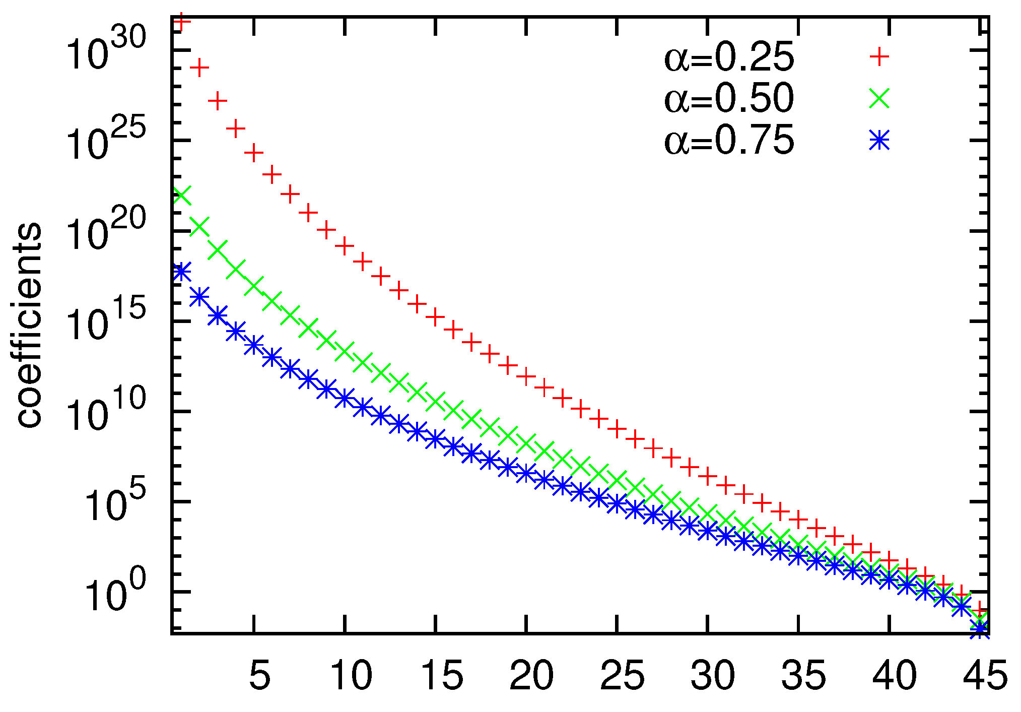
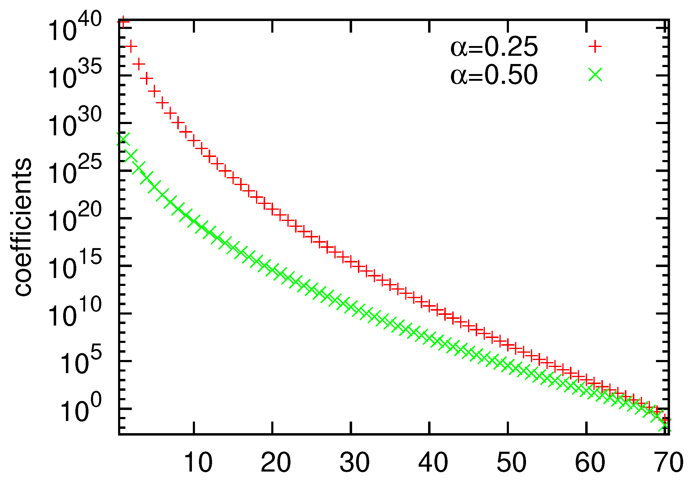
In Figure 2 and Figure 3, we illustrate the behavior of the poles ${\tilde{d}}_i$ of ${\tilde{r}}_{\alpha ,k}\left(z\right)$ in (25), where $\alpha \in \{\frac{1}{4},\frac{1}{2},\frac{3}{4}\}$ and $k=45,70$, respectively.

One can see that for $k=45$, the first part of the poles for $\alpha =\frac{1}{4},\frac{1}{2}$ consists of extremely large values (for $\alpha =\frac{1}{4}$ first nine coefficients are bigger than ${10}^{20}$). For $k=70$ the situation is: first 21 coefficients are bigger than ${10}^{20}$ for $\alpha =\frac{1}{4}$ and for $\alpha =\frac{1}{2}$ eight coefficients are bigger than ${10}^{20}$. Furthermore, the asymptotic of the poles clustering towards $-\infty$, based on Theorem 1(c), is also well represented, as the order of the first pole for $\alpha =1/4$ is approximately $\sqrt{1/2}/\sqrt{1/4}=\sqrt{2}$ times larger than the order of the first pole for $\alpha =1/2$ and approximately $\sqrt{3/4}/\sqrt{1/4}=\sqrt{3}$ times larger than the order of the first pole for $\alpha =3/4$.

For extremely large values of $-{\tilde{d}}_i$, the condition number of the matrices $\mathbb{A}-{\lambda }_{1,h}{\tilde{d}}_i\mathbb{I}$, involved in (13), is practically equal to one. Of course, we do not need any preconditioning for such well-conditioned matrices. Moreover, even solving such systems may not be the right approach. This motivates us to investigate potential reduction on the number of linear systems to be solved without losing BURA accuracy.

Let $\ell <k$ be chosen such that $|{\tilde{d}}_i|$ is very large for $i=1,\dots ,\ell$. Then we can define the following rational approximations of $z^{-\alpha }$, both of degree $k-\ell$:

$$\begin{array}{cc}\hfill {\tilde{r}}_{\alpha ,k,\ell }^A\left(z\right)& =E_{\alpha ,k}-\sum _{i=1}^{\ell }\frac{{\tilde{c}}_i}{{\tilde{d}}_i}+\sum _{i=\ell +1}^k\frac{{\tilde{c}}_i}{z-{\tilde{d}}_i},\hfill \\ \hfill {\tilde{r}}_{\alpha ,k,\ell }^M\left(z\right)& =E_{\alpha ,k}\prod _{i=1}^{\ell }\frac{{\tilde{\xi }}_i}{{\tilde{d}}_i}\prod _{i=\ell +1}^k\frac{z-{\tilde{\xi }}_i}{z-{\tilde{d}}_i}.\hfill \end{array}$$

Lemma 3.

The following relations hold true for every $\alpha \in (0,1)$, $k\in \mathbb{N}$, and $z\in [1,\infty )$:

$${\tilde{r}}_{\alpha ,k,0}^A\left(z\right)\equiv {\tilde{r}}_{\alpha ,k}\left(z\right)\equiv {\tilde{r}}_{\alpha ,k,0}^M\left(z\right);{\tilde{r}}_{\alpha ,k,k}^A\left(z\right)\equiv c_0\equiv {\tilde{r}}_{\alpha ,k,k}^M\left(z\right);{\tilde{r}}_{\alpha ,k,\ell }^A\left(z\right)<{\tilde{r}}_{\alpha ,k,\ell }^M\left(z\right),$$

for all intermediate values $\ell =1,\cdots ,k-1$.

Proof. 

The first two relations ${\tilde{r}}_{\alpha ,k,\ell }^A\left(z\right)\equiv {\tilde{r}}_{\alpha ,k,\ell }^M\left(z\right)$ for $\ell =0,k$ are trivial. Now, let $\ell =1,\cdots ,k-1$ be fixed. First we show that ${lim}_{k\to \infty }{\tilde{r}}_{\alpha ,k,\ell }^A\left(z\right)<{lim}_{k\to \infty }{\tilde{r}}_{\alpha ,k,\ell }^M\left(z\right)$. Indeed, following the notation from Section 4.1 let us define

$${\overline{r}}_{\alpha ,k,\ell }^A\left(t\right):=c_0+\sum _{i=\ell +1}^k\frac{c_i}{t-d_i}\mathrm{and}{\overline{r}}_{\alpha ,k,\ell }^M\left(t\right):=c_0\prod _{i=\ell +1}^k\frac{t-{\xi }_i}{t-d_i}=c_0+\sum _{i=\ell +1}^k\frac{{\overline{c}}_i}{t-d_i}.$$

Then ${\tilde{c}}_0^A:={lim}_{z\to \infty }{\tilde{r}}_{\alpha ,k,\ell }^A\left(z\right)={\overline{r}}_{\alpha ,k,\ell }^A\left(0\right)$, while ${\tilde{c}}_0^M:={lim}_{z\to \infty }{\tilde{r}}_{\alpha ,k,\ell }^M\left(z\right)={\overline{r}}_{\alpha ,k,\ell }^M\left(0\right)$. Applying (23), we obtain

$$c_i={\overline{c}}_i\prod _{j=1}^{\ell }\frac{d_i-{\xi }_j}{d_i-d_j}<{\overline{c}}_i,\forall i=\ell +1,\cdots ,k,$$

since $c_i,{\overline{c}}_i<0$ and $(d_i-{\xi }_j)/(d_i-d_j)>1$ for $j<i$ due to (17). Therefore

$$\underset{z\to \infty }{lim}({\tilde{r}}_{\alpha ,k,\ell }^A\left(z\right)-{\tilde{r}}_{\alpha ,k,\ell }^M\left(z\right))=\sum _{i=l+1}^k\frac{{\overline{c}}_i-c_i}{d_i}<0.$$

Next, via expressing the two functions in the form

$${\tilde{r}}_{\alpha ,k,\ell }^A\left(z\right)={\tilde{c}}_0^A+\sum _{i=\ell +1}^k\frac{{\tilde{c}}_i}{z-{\tilde{d}}_i},\mathrm{respectively}{\tilde{r}}_{\alpha ,k,\ell }^M\left(z\right)={\tilde{c}}_0^M+\sum _{i=\ell +1}^k\frac{{\tilde{c}}_i^M}{z-{\tilde{d}}_i},$$

and applying (23) one more time, we conclude that for all $0<\ell <k$ and every $i=\ell +1,\cdots ,k$

$${\tilde{c}}_i=\left(\frac{E_{\alpha ,k}}{{\tilde{c}}_0^M}\prod _{j=1}^{\ell }\frac{{\tilde{d}}_i-{\tilde{\xi }}_j}{{\tilde{d}}_i-{\tilde{d}}_j}\right){\tilde{c}}_i^M=\prod _{j=1}^{\ell }\left(\frac{{\tilde{d}}_j}{{\tilde{\xi }}_j}\frac{{\tilde{d}}_i-{\tilde{\xi }}_j}{{\tilde{d}}_i-{\tilde{d}}_j}\right){\tilde{c}}_i^M>{\tilde{c}}_i^M,$$

due to (27) and ${\tilde{c}}_i,{\tilde{c}}_i^M>0$. Finally, for the function

$$e\left(z\right):={\tilde{r}}_{\alpha ,k,\ell }^A\left(z\right)-{\tilde{r}}_{\alpha ,k,\ell }^M\left(z\right)={\tilde{c}}_0^A-{\tilde{c}}_0^M+\sum _{i=\ell +1}^k\frac{{\tilde{c}}_i-{\tilde{c}}_i^M}{z-{\tilde{d}}_i},$$

we know that

$$e\left(0\right)=c_0-c_0=0;e^{\prime }\left(z\right)=-\sum _{i=\ell +1}^k\frac{{\tilde{c}}_i-{\tilde{c}}_i^M}{{(z-{\tilde{d}}_i)}^2}<0\Rightarrow e\left(z\right)<0,z>0.$$

The proof is completed. □

Let $\delta <1$ be given. We can then introduce the error indicators

$${\tilde{E}}_{\alpha ,k,\ell }^{A,\delta }=\underset{z\in [1,{\delta }^{-1}]}{max}|z^{-\alpha }-{\tilde{r}}_{\alpha ,k,\ell }^A\left(z\right)|,{\tilde{E}}_{\alpha ,k,\ell }^{M,\delta }=\underset{z\in [1,{\delta }^{-1}]}{max}|z^{-\alpha }-{\tilde{r}}_{\alpha ,k,\ell }^M\left(z\right)|.$$

Both functions ${\tilde{r}}_{\alpha ,k,\ell }^A$ and ${\tilde{r}}_{\alpha ,k,\ell }^M$ share the same poles and the error analysis performed later in this section indicates that both reduction procedures could be used in practical applications. They do not only stabilize the numerical computations but also improve the efficiency of the BURA solver.

Motivated by the above observation, we replace the ${\tilde{r}}_{\alpha ,k}\left(\mathbb{A}\right)$ in the BURA method for solving the spectral fractional elliptic Equation (1) by either ${\tilde{r}}_{\alpha ,k,\ell }^A\left(\mathbb{A}\right)$ or ${\tilde{r}}_{\alpha ,k,\ell }^M\left(\mathbb{A}\right)$ and obtain the following BURA-AR and BURA-MR formulations

$$\begin{array}{cc}\hfill {\mathbf{u}}_{k,\ell }^A& ={\lambda }_{1,h}^{-\alpha }\left[\left(E_{\alpha ,k}-\sum _{i=1}^{\ell }\frac{{\tilde{c}}_i}{{\tilde{d}}_i}\right)\mathbb{I}+\sum _{i=\ell +1}^k\left({\lambda }_{1,h}{\tilde{c}}_i\right){(\mathbb{A}-{\lambda }_{1,h}{\tilde{d}}_i\mathbb{I})}^{-1}\right]\mathbf{f};\hfill \\ \hfill {\mathbf{u}}_{k,\ell }^M& ={\lambda }_{1,h}^{-\alpha }{E}_{\alpha ,k}\prod _{i=1}^{\ell }\frac{{\tilde{\xi }}_i}{{\tilde{d}}_i}\prod _{i=\ell +1}^k\left[(\mathbb{A}-{\lambda }_{1,h}{\tilde{\xi }}_i\mathbb{I}){(\mathbb{A}-{\lambda }_{1,h}{\tilde{d}}_i\mathbb{I})}^{-1}\right]\mathbf{f}.\hfill \end{array}$$

(28)

Using the BURA-AR and BURA-MR methods, we reduce the number of linear systems that are to be solved from k to $k-\ell$, and thus we decrease the computational complexity of the method.

5.1. BURA-AR Error Analysis

Throughout this section, let $\delta$, $\alpha$, and k be fixed. We are interested in analyzing the error indicator ${\tilde{E}}_{\alpha ,k,\ell }^{A,\delta }$. By triangle inequality, we have

$${\tilde{E}}_{\alpha ,k,\ell }^{A,\delta }\le \underset{z\in [1,{\delta }^{-1}]}{max}\left(|z^{-\alpha }-{\tilde{r}}_{\alpha ,k}\left(z\right)|+|{\tilde{r}}_{\alpha ,k,\ell }^A\left(z\right)-{\tilde{r}}_{\alpha ,k}\left(z\right)|\right)\le E_{\alpha ,k}+\underset{z\in [1,{\delta }^{-1}]}{max}|{\tilde{r}}_{\alpha ,k,\ell }^A\left(z\right)-{\tilde{r}}_{\alpha ,k}\left(z\right)|,$$

so we need to estimate the second term. Applying (27) and Lemma 2, we derive

$$\begin{array}{cc}\hfill {\tilde{r}}_{\alpha ,k,\ell }^A\left(z\right)-{\tilde{r}}_{\alpha ,k}\left(z\right)& =\sum _{i=1}^l\left[-\frac{{\tilde{c}}_i}{{\tilde{d}}_i}-\frac{{\tilde{c}}_i}{z-{\tilde{d}}_i}\right]=\sum _{i=1}^{\ell }-\frac{{\tilde{c}}_i}{{\tilde{d}}_i}\frac{z}{z-{\tilde{d}}_i}\hfill \\ \hfill & =\sum _{i=1}^{\ell }\frac{c_i}{d_i}\frac{d_{i}z}{d_{i}z-1}<2\sum _{i=1}^{\ell }\frac{|d_i{|}^{1+\alpha }z}{|d_i|z+1}\hfill \\ \hfill & <2\sum _{i=1}^{\ell }|d_i{|}^{1+\alpha }z<2\ell {\left|d_{\ell }\right|}^{1+\alpha }z.\hfill \end{array}$$

Hence, we proved the following theorem:

Theorem 2.

Let $\delta ,\alpha \in (0,1)$ and $k\in \mathbb{N}$. If $\ell \in \mathbb{N}$, such that $|d_{\ell }|\le 1$, then

$${\tilde{E}}_{\alpha ,k,\ell }^{A,\delta }\le E_{\alpha ,k}+2\ell {\left|d_{\ell }\right|}^{1+\alpha }{\delta }^{-1}.$$

As a byproduct, we also derived that whenever $\delta <{\eta }_{2k+1}$

$$\begin{array}{ccc}\hfill E_{\alpha ,k}={\tilde{E}}_{\alpha ,k,0}^{A,\delta }<{\tilde{E}}_{\alpha ,k,\ell }^{A,\delta }& <{\tilde{E}}_{\alpha ,k,{\ell }^{\prime }}^{A,\delta }<{\tilde{E}}_{\alpha ,k,k}^{A,\delta }=c_0-{\delta }^{\alpha },\hfill & \hfill \forall 0<\ell <{\ell }^{\prime }<k;\\ \hfill {\tilde{E}}_{\alpha ,k,\ell }^{A,\delta }& <{\tilde{E}}_{\alpha ,k,{\ell }^{\prime }}^{A,{\delta }^{\prime }},\hfill & \hfill \forall 0<{\delta }^{\prime }<\delta <{\tilde{\eta }}_{2k+1},\end{array}$$

(29)

meaning that for fixed $\alpha$ and k, the error indicator ${\tilde{E}}_{\alpha ,k,\ell }^{A,\delta }$ is a monotonically increasing function with respect to ℓ and a monotonically decreasing function with respect to $\delta$. The proof relies on the observation that ${\tilde{r}}_{\alpha ,k,{\ell }^{\prime }}^A\left(z\right)-{\tilde{r}}_{\alpha ,k,\ell }^A\left(z\right)>0$, $z>0$, proven in an identical way as ${\tilde{r}}_{\alpha ,k,\ell }^A\left(z\right)-{\tilde{r}}_{\alpha ,k}\left(z\right)>0$ above, together with (27) and (18) that imply

$${\tilde{\epsilon }}_{\alpha ,k,\ell }^A\left({\tilde{\eta }}_{2k+1}\right)-E_{\alpha ,k}={\tilde{\epsilon }}_{\alpha ,k,\ell }^A\left({\tilde{\eta }}_{2k+1}\right)-{\tilde{\epsilon }}_{\alpha ,k}\left({\tilde{\eta }}_{2k+1}\right)={\tilde{r}}_{\alpha ,k}\left({\tilde{\eta }}_{2k+1}\right)-{\tilde{r}}_{\alpha ,k,\ell }^A\left({\tilde{\eta }}_{2k+1}\right)>0.$$

Note that while $\lceil {log}_{10}(2\ell |d_{\ell }{|}^{1+\alpha }{\delta }^{-1})\rceil \le \lfloor {log}_{10}\left(E_{\alpha ,k}\right)\rfloor$, the reduction error between the BURA-AR method and the original BURA method is dominated by the BURA approximation error $E_{\alpha ,k}$, thus the reduction process does not affect the overall accuracy of the solver in any way. In practice, we observe that due to the large difference in the orders of $|d_i|$ for small i, the multiplier l can be omitted and

$$\sum _{i=1}^{\ell }|d_i{|}^{1+\alpha }\sim {\left|d_{\ell }\right|}^{1+\alpha }.$$

Corollary 2.

Let $\mathbf{u}$ be the solution of the linear algebraic system (3) and ${\mathbf{u}}_{k,\ell }^A$ be the additive reduced BURA solution, corresponding to (28) with $|d_{\ell }|\le 1$. Then

$${∥\mathbf{u}-{\mathbf{u}}_{k,\ell }^A∥}_2<\left(E_{\alpha ,k}+2\ell {\left|d_{\ell }\right|}^{1+\alpha }\frac{{\lambda }_{N,h}}{{\lambda }_{1,h}}\right){\parallel \mathbf{f}\parallel }_2.$$

Example 1.

Consider the fractional Laplacian problem with homogeneous Dirichlet boundary conditions in the d dimensional unit cube, $d\in \{1,2,3\}$. Take the finite difference or lumped finite element discretization of the problem on a uniform mesh with mesh-size h. It is well-known that the condition number of the matrix $\mathbb{A}$ generated in this way for the corresponding algebraic Equation (3) behaves like

$$\kappa \left(\mathbb{A}\right)=\frac{{\lambda }_{N,h}}{{\lambda }_{1,h}}\approx h^{-2},$$

independent of the space dimensionality of the problem. According to (8), in order to balance the discretization and the approximation BURA error, there is no practical point to take larger k than the one that guarantees $E_{\alpha ,k}=h^{-2}$. Now, in order to balance the reduction error with the approximation one, applying Corollary 2, we conclude that all systems, corresponding to diagonal shifts ${\tilde{d}}_i$, such that

$$|{\tilde{d}}_i|\gtrsim h^{-\frac{4}{1+\alpha }},\forall \alpha \in (0,1),$$

(30)

can be reduced in the numerical computation. Here, following (27), we used that ${\tilde{d}}_i=1/d_i$. In particular, for $\alpha =0.25$ and $h={10}^{-2},{10}^{-3},{10}^{-4}$ we can reduce all systems corresponding to diagonal shifts that are higher or equal to ${10}^7,{10}^{10},{10}^{13}$, respectively. The results are summarized in

Table 1. Reduction possibilities for the homogeneous fractional Laplacian problem in the vicinity of the theoretical estimate (30).

$\mathit{\alpha }$	h	$\mathit{k}=min\{\mathit{s}:{\mathit{E}}_{\mathit{\alpha },\mathit{s}}<{\mathit{h}}^2\}$	$\mathit{\ell }=\#\{\mathit{i}:|{\tilde{\mathit{d}}}_{\mathit{i}}|\gtrsim {\mathit{h}}^{-\frac{4}{1+\mathit{\alpha }}}\}$
$0.25$	${10}^{-2}$	12	4
	${10}^{-3}$	24	9
	${10}^{-4}$	40	15
	${10}^{-5}$	61	23
$0.5$	${10}^{-2}$	7	1
	${10}^{-3}$	13	2
	${10}^{-4}$	21	2
	${10}^{-5}$	32	3
$0.75$	${10}^{-2}$	4	0
	${10}^{-3}$	9	0
	${10}^{-4}$	14	0
	${10}^{-5}$	21	0

. We observe that the BURA-AR method can reduce more than $1/3$ of the systems to be solved without influencing the overall BURA error order when $\alpha =0.25$. As α increases, the impact of BURA-AR on the computational efficiency decreases. Thus, for the considered example, the results in Table 1 show that for $\alpha =0.75$, the recommended reduction is $\ell =0$. This is in agreement with the significantly higher accuracy of BURA for $\alpha =0.75$, see Figure 1. In other words, smaller k is needed to ensure a certain accuracy, and then a smaller reduction is applicable.

Furthermore, for every $\alpha \in (0,1)$, we can reduce all systems with diagonal shifts larger than ${10}^{16}$, as long as $h\ge {10}^{-4}$, which usually holds true in practical applications.

5.2. BURA-MR Error Analysis

Again, let $\delta$, $\alpha$, and k be fixed. We are interested in analyzing the error indicator ${\tilde{E}}_{\alpha ,k,\ell }^{M,\delta }$. By triangle inequality, we have

$${\tilde{E}}_{\alpha ,k,\ell }^{M,\delta }\le E_{\alpha ,k}+\sum _{s=0}^{l-1}\underset{z\in [1,{\delta }^{-1}]}{max}|{\tilde{r}}_{\alpha ,k,s+1}^M\left(z\right)-{\tilde{r}}_{\alpha ,k,s}^M\left(z\right)|,$$

where ${\tilde{r}}_{\alpha ,k,0}^M\equiv {\tilde{r}}_{\alpha ,k}$. Since

$${\tilde{r}}_{\alpha ,k,s+1}^M\left(z\right)-{\tilde{r}}_{\alpha ,k,s}^M\left(z\right)={\tilde{r}}_{\alpha ,k,s}^M\left(z\right)\left[\left(\frac{{\tilde{\xi }}_{s+1}}{{\tilde{d}}_{s+1}}-1\right)\frac{z}{z-{\tilde{\xi }}_{s+1}}\right]>0,$$

${\tilde{\xi }}_{s+1}/{\tilde{d}}_{s+1}-1=d_{s+1}/{\xi }_{s+1}-1>0$ (see (27)), and $1/(z-{\tilde{\xi }}_{s+1})$ is strictly monotonically increasing for $z\in [1,\infty )$ we conclude that

$$\begin{array}{cc}\hfill \underset{z\in [1,{\delta }^{-1}]}{max}|{\tilde{r}}_{\alpha ,k,s+1}^M\left(z\right)-{\tilde{r}}_{\alpha ,k,s}^M\left(z\right)|& <\underset{z\in [1,{\delta }^{-1}]}{max}z{\tilde{r}}_{\alpha ,k,s}^M\left(z\right)\left(\frac{d_{s+1}-{\xi }_{s+1}}{{\xi }_{s+1}}\frac{{\xi }_{s+1}}{{\tilde{\xi }}_{s+1}-1}\right)\hfill \\ \hfill & <\underset{z\in [1,{\delta }^{-1}]}{max}z{\tilde{r}}_{\alpha ,k,k}^M\left(z\right)({\xi }_{s+1}-d_{s+1})={\delta }^{-1}{c}_0({\xi }_{s+1}-d_{s+1})\hfill \\ \hfill & <2\prod _{j>s}\frac{d_s-d_j}{d_s-{\xi }_j}|d_s{|}^{1+\alpha }{\delta }^{-1}=2C(k,s){\left|d_s\right|}^{1+\alpha }{\delta }^{-1},\hfill \end{array}$$

where the constants

$$C(k,s)\le C(k,1)=\prod _{j=2}^k\frac{d_1-d_j}{d_1-{\xi }_j}<\infty ,$$

are uniformly bounded for fixed k. Moreover, (19) suggests that the zeros and the poles of $r_{\alpha ,k}\left(t\right)$ are grouped into pairs, meaning that $|d_s-{\xi }_{s+1}|>{\xi }_{s+1}-d_{s+1}$, thus

$$\frac{d_s-d_j}{d_s-{\xi }_j}\le \frac{d_s-d_{s+1}}{d_s-{\xi }_{s+1}}<\frac{(2{\xi }_{s+1}-d_{s+1})-d_{s+1}}{(2{\xi }_{s+1}-d_{s+1})-{\xi }_{s+1}}=2,$$

and $C(k,s)<2^{k-s}$. Analogously to Section 5.1, we proved the following theorem:

Theorem 3.

Let $\delta ,\alpha \in (0,1)$ and $k\in \mathbb{N}$. If $\ell \in \mathbb{N}$, such that $|d_{\ell }|\le 1$, then

$${\tilde{E}}_{\alpha ,k,\ell }^{M,\delta }\le E_{\alpha ,k}+2\ell C{\left|d_{\ell }\right|}^{1+\alpha }{\delta }^{-1},$$

where the constant $C<+\infty$ depends solely on k.

Again, as a byproduct, we also derived that whenever $\delta <{\eta }_{2k+1}$

$$\begin{array}{ccc}\hfill E_{\alpha ,k}={\tilde{E}}_{\alpha ,k,0}^{M,\delta }<{\tilde{E}}_{\alpha ,k,\ell }^{M,\delta }& <{\tilde{E}}_{\alpha ,k,{\ell }^{\prime }}^{M,\delta }<{\tilde{E}}_{\alpha ,k,k}^{M,\delta }=c_0-{\delta }^{\alpha },\hfill & \hfill \forall 0<\ell <{\ell }^{\prime }<k;\\ \hfill {\tilde{E}}_{\alpha ,k,\ell }^{M,\delta }& <{\tilde{E}}_{\alpha ,k,{\ell }^{\prime }}^{M,{\delta }^{\prime }},\hfill & \hfill \forall 0<{\delta }^{\prime }<\delta <{\tilde{\eta }}_{2k+1},\end{array}$$

(31)

meaning that for fixed $\alpha$ and k, the error indicator ${\tilde{E}}_{\alpha ,k,\ell }^{M,\delta }$ is a monotonically increasing function with respect to ℓ and a monotonically decreasing function with respect to $\delta$.

Corollary 3.

Let $\mathbf{u}$ be the solution of the linear algebraic system (3) and ${\mathbf{u}}_{k,\ell }^M$ be the multiplicative reduced BURA solution, corresponding to (28) with $|d_{\ell }|\le 1$. Then

$${∥\mathbf{u}-{\mathbf{u}}_{k,\ell }^M∥}_2<\left(E_{\alpha ,k}+2\ell C{\left|d_{\ell }\right|}^{1+\alpha }\frac{{\lambda }_{N,h}}{{\lambda }_{1,h}}\right){\parallel \mathbf{f}\parallel }_2.$$

5.3. BURA-AR and BURA-MR Comparison

To summarize, the following theoretical estimates and relations were established in Section 5:

Theorem 4.

Let $\alpha \in (0,1)$ and $k\in \mathbb{N}$. Consider the BURA element $r_{\alpha ,k}\left(t\right)$ and take arbitrary $0<\delta <{\eta }_{2k+1}$, where ${\eta }_{2k+1}$ is the extreme point of ${\epsilon }_{\alpha ,k}\left(t\right)$ before 1. Then

$$\begin{array}{c}\hfill {\tilde{r}}_{\alpha ,k}\left(z\right)<{\tilde{r}}_{\alpha ,k,1}^A<{\tilde{r}}_{\alpha ,k,2}^A<\cdots <{\tilde{r}}_{\alpha ,k,k-1}^A<c_0\\ \hfill {\tilde{r}}_{\alpha ,k}\left(z\right)<{\tilde{r}}_{\alpha ,k,1}^M<{\tilde{r}}_{\alpha ,k,2}^M<\cdots <{\tilde{r}}_{\alpha ,k,k-1}^M<c_0\\ \hfill {\tilde{r}}_{\alpha ,k,\ell }^A\left(z\right)<{\tilde{r}}_{\alpha ,k,\ell }^M\left(z\right),\forall \ell =1,\cdots ,k-1\\ \hfill E_{\alpha ,k}<{\tilde{E}}_{\alpha ,k,1}^{A,\delta }<{\tilde{E}}_{\alpha ,k,2}^{A,\delta }<\cdots <{\tilde{E}}_{\alpha ,k,k-1}^{A,\delta }<c_0-{\delta }^{\alpha }\\ \hfill E_{\alpha ,k}<{\tilde{E}}_{\alpha ,k,1}^{M,\delta }<{\tilde{E}}_{\alpha ,k,2}^{M,\delta }<\cdots <{\tilde{E}}_{\alpha ,k,k-1}^{M,\delta }<c_0-{\delta }^{\alpha }\\ \hfill {\tilde{E}}_{\alpha ,k,\ell }^{A,\delta }\left(z\right)<{\tilde{E}}_{\alpha ,k,\ell }^{M,\delta }\left(z\right),\forall \ell =1,\cdots ,k-1.\end{array}$$

Therefore, from a theoretical approximating point of view, the BURA-AR method always outperforms the BURA-MR method, giving rise to smaller errors for a fixed number of systems to be solved. Furthermore, in the BURA-MR method, apart from the $k-\ell$ algebraic systems, there are also $k-\ell$ matrix-vector multiplications (see (28)). On top of that, the BURA-AR method allows for parallel, independent solutions of the algebraic systems, while the BURA-MR method is a sequential one, as the solution of the previous system becomes the right-hand side of the next one.

However, due to the interlacing property (17) and (27), the BURA-MR method seems to be numerically stable, independently of the value of ℓ. Moreover, based on the conducted numerical experiments, we observe that the difference ${\tilde{E}}_{\alpha ,k,\ell }^{M,\delta }\left(z\right)-{\tilde{E}}_{\alpha ,k,\ell }^{A,\delta }\left(z\right)$ decays as ℓ increases, so from an application point of view, the two methods are equally useful. This topic will be addressed in the next section, where various experimental data are generated and analyzed.

6. Numerical Experiments

In this section, two classes of numerical experiments are considered. The first one aims at numerical validation of the theoretical foundations for the error indicator ${\tilde{E}}_{\alpha ,k,\ell }^{A,\delta }$, derived in Section 5. Therefore, the experiments are in 1D and involve numerical and visual comparison of $z^{-\alpha }$ and ${\tilde{r}}_{\alpha ,k,\ell }^A\left(z\right)$ in the interval $z\in [1,{\delta }^{-1})$. A large value for k, namely $k=70$ is considered so that the reduction benefits of BURA-AR are better illustrated. The decreasing effect of BURA-AR when $\alpha$ increases has already been commented on; therefore, the focus here is mostly on $\alpha =\{0.25,0.5\}$. Here, and in what follows, the case $\alpha =0.75$ and $k=45$ are included for completeness. The numerical data are summarized in

Table 2. The accuracy ${\tilde{E}}_{\alpha ,k,\ell }^{A,\delta }$ for $\alpha =0.25,0.5,0.75$.

	$\mathit{k}=70$				$\mathit{k}=45$
ℓ	$\mathbf{\alpha }=\mathbf{0}.\mathbf{25}$		$\mathbf{\alpha }=\mathbf{0}.\mathbf{5}$		$\mathbf{\alpha }=\mathbf{0}.\mathbf{75}$
	$\mathbf{\delta }={\mathbf{10}}^{-\mathbf{8}}$	$\mathbf{\delta }={\mathbf{10}}^{-\mathbf{12}}$	$\mathbf{\delta }={\mathbf{10}}^{-\mathbf{8}}$	$\mathbf{\delta }={\mathbf{10}}^{-\mathbf{12}}$	$\mathbf{\delta }={\mathbf{10}}^{-\mathbf{8}}$	$\mathbf{\delta }={\mathbf{10}}^{-\mathbf{12}}$
0	$1.434\times {10}^{-11}$	$1.434\times {10}^{-11}$	$5.345\times {10}^{-16}$	$5.346\times {10}^{-16}$	$9.944\times {10}^{-16}$	$9.944\times {10}^{-16}$
1	$1.434\times {10}^{-11}$	$1.434\times {10}^{-11}$	$5.345\times {10}^{-16}$	$5.346\times {10}^{-16}$	$9.944\times {10}^{-16}$	$9.945\times {10}^{-16}$
2	$1.434\times {10}^{-11}$	$1.434\times {10}^{-11}$	$5.339\times {10}^{-16}$	$5.346\times {10}^{-16}$	$9.944\times {10}^{-16}$	$1.003\times {10}^{-15}$
3	$1.434\times {10}^{-11}$	$1.434\times {10}^{-11}$	$5.339\times {10}^{-16}$	$5.346\times {10}^{-16}$	$9.944\times {10}^{-16}$	$1.454\times {10}^{-15}$
4	$1.434\times {10}^{-11}$	$1.434\times {10}^{-11}$	$5.339\times {10}^{-16}$	$5.346\times {10}^{-16}$	$9.954\times {10}^{-16}$	$2.184\times {10}^{-14}$
5	$1.434\times {10}^{-11}$	$1.434\times {10}^{-11}$	$5.339\times {10}^{-16}$	$5.346\times {10}^{-16}$	$1.014\times {10}^{-15}$	$4.305\times {10}^{-13}$
6	$1.434\times {10}^{-11}$	$1.434\times {10}^{-11}$	$5.339\times {10}^{-16}$	$5.346\times {10}^{-16}$	$1.356\times {10}^{-15}$	$5.856\times {10}^{-12}$
7	$1.434\times {10}^{-11}$	$1.434\times {10}^{-11}$	$5.339\times {10}^{-16}$	$5.346\times {10}^{-16}$	$8.247\times {10}^{-15}$	$5.436\times {10}^{-11}$
8	$1.434\times {10}^{-11}$	$1.434\times {10}^{-11}$	$5.345\times {10}^{-16}$	$5.346\times {10}^{-16}$	$7.553\times {10}^{-14}$	$3.123\times {10}^{-10}$
9	$1.434\times {10}^{-11}$	$1.434\times {10}^{-11}$	$5.345\times {10}^{-16}$	$5.346\times {10}^{-16}$	$6.478\times {10}^{-13}$	$1.172\times {10}^{-09}$
10	$1.434\times {10}^{-11}$	$1.434\times {10}^{-11}$	$5.345\times {10}^{-16}$	$5.354\times {10}^{-16}$	$4.983\times {10}^{-12}$	$3.391\times {10}^{-09}$
11	$1.434\times {10}^{-11}$	$1.434\times {10}^{-11}$	$5.345\times {10}^{-16}$	$5.410\times {10}^{-16}$	$3.467\times {10}^{-11}$	$8.497\times {10}^{-09}$
12	$1.434\times {10}^{-11}$	$1.434\times {10}^{-11}$	$5.345\times {10}^{-16}$	$5.805\times {10}^{-16}$	$2.200\times {10}^{-10}$	$1.959\times {10}^{-08}$
13	$1.434\times {10}^{-11}$	$1.434\times {10}^{-11}$	$5.345\times {10}^{-16}$	$8.361\times {10}^{-16}$	$1.275\times {10}^{-09}$	$4.281\times {10}^{-08}$
14	$1.434\times {10}^{-11}$	$1.434\times {10}^{-11}$	$5.348\times {10}^{-16}$	$3.319\times {10}^{-15}$	$6.644\times {10}^{-09}$	$8.999\times {10}^{-08}$
15	$1.434\times {10}^{-11}$	$1.434\times {10}^{-11}$	$5.363\times {10}^{-16}$	$1.933\times {10}^{-14}$	$3.011\times {10}^{-08}$	$3.650\times {10}^{-07}$
16	$1.434\times {10}^{-11}$	$1.434\times {10}^{-11}$	$5.446\times {10}^{-16}$	$1.045\times {10}^{-13}$	$1.133\times {10}^{-07}$	$3.650\times {10}^{-07}$
17	$1.434\times {10}^{-11}$	$1.434\times {10}^{-11}$	$5.864\times {10}^{-16}$	$5.352\times {10}^{-13}$	$3.462\times {10}^{-07}$	$7.102\times {10}^{-07}$
18	$1.434\times {10}^{-11}$	$1.434\times {10}^{-11}$	$7.889\times {10}^{-16}$	$2.613\times {10}^{-12}$	$8.829\times {10}^{-07}$	$1.355\times {10}^{-06}$
19	$1.434\times {10}^{-11}$	$1.434\times {10}^{-11}$	$1.739\times {10}^{-15}$	$1.221\times {10}^{-11}$	$1.974\times {10}^{-06}$	$2.540\times {10}^{-06}$
20	$1.434\times {10}^{-11}$	$1.434\times {10}^{-11}$	$6.009\times {10}^{-15}$	$5.480\times {10}^{-11}$	$4.039\times {10}^{-06}$	$4.684\times {10}^{-06}$
21	$1.434\times {10}^{-11}$	$1.435\times {10}^{-11}$	$2.430\times {10}^{-14}$	$2.364\times {10}^{-10}$	$7.801\times {10}^{-06}$	$8.509\times {10}^{-06}$
22	$1.434\times {10}^{-11}$	$1.437\times {10}^{-11}$	$1.000\times {10}^{-13}$	$9.802\times {10}^{-10}$	$1.448\times {10}^{-05}$	$1.524\times {10}^{-05}$
23	$1.434\times {10}^{-11}$	$1.449\times {10}^{-11}$	$4.039\times {10}^{-12}$	$3.882\times {10}^{-09}$	$2.616\times {10}^{-05}$	$2.696\times {10}^{-05}$
24	$1.434\times {10}^{-11}$	$1.511\times {10}^{-11}$	$1.587\times {10}^{-12}$	$1.446\times {10}^{-08}$	$4.627\times {10}^{-05}$	$4.710\times {10}^{-05}$
25	$1.434\times {10}^{-11}$	$2.228\times {10}^{-11}$	$6.068\times {10}^{-12}$	$4.916\times {10}^{-08}$	$8.049\times {10}^{-05}$	$8.136\times {10}^{-05}$
26	$1.434\times {10}^{-11}$	$5.806\times {10}^{-11}$	$2.260\times {10}^{-11}$	$1.461\times {10}^{-07}$	$1.381\times {10}^{-04}$	$1.390\times {10}^{-04}$
27	$1.435\times {10}^{-11}$	$2.209\times {10}^{-10}$	$8.210\times {10}^{-11}$	$3.683\times {10}^{-07}$	$2.343\times {10}^{-04}$	$2.352\times {10}^{-04}$
28	$1.440\times {10}^{-11}$	$9.415\times {10}^{-10}$	$2.913\times {10}^{-10}$	$7.929\times {10}^{-07}$	$3.932\times {10}^{-04}$	$3.941\times {10}^{-04}$
29	$1.460\times {10}^{-11}$	$4.048\times {10}^{-09}$	$1.010\times {10}^{-09}$	$1.509\times {10}^{-06}$	$6.536\times {10}^{-04}$	$6.545\times {10}^{-04}$

.

For $\alpha =0.25$, $k=70$ and $\delta ={10}^{-12}$ the accuracy remains the same for all values of ℓ in the interval $[0,20]$. The error doubles around $\ell =25$ and then starts to exponentially grow. Such a behavior perfectly agrees with Theorem 2 and experimentally confirms that as long as $|d_{\ell }{|}^{1+\alpha }{\delta }^{-1}\precsim E_{\alpha ,k}$, the reduction process does not affect the order of ${\tilde{E}}_{\alpha ,k,\ell }^{A,\delta }$. Indeed, we have that $E_{0.25,70}\approx {10}^{-11}$, thus for $|d_{\ell }|\le {10}^{-23·4/5}\le {10}^{-19}$ we should be safe. Checking the poles of $r_{0.25,70}$ we get that $d_{\ell }<{10}^{-19}$ for $\ell \le 23$, while $|d_{\ell }|=O\left({10}^{-18}\right)$ for $\ell =\{24,25\}$. For $\alpha =\frac{1}{4}$ and $\delta ={10}^{-8}$ the accuracy is not changed for all values of ℓ in the interval $[0,29]$. Again, this corresponds to $|d_{\ell }|\le {10}^{-19·4/5}\le {10}^{-16}$, which holds true for all $\ell \le 28$.

For $\alpha =0.5$ and $k=70$, the observations are the same. For $\delta ={10}^{-12}$, as long as $|d_{\ell }|\le {10}^{-27.5·2/3}={10}^{-55/3}$, the reduction does not affect the overall accuracy. This relation holds true for $\ell \le 9$. Then $|d_{\ell }|=O\left({10}^{-19}\right)$ for $\ell =\{10,11\}$ and ${\tilde{E}}_{\alpha ,k,\ell }^{A,\delta }$ slowly increases. Finally, from the moment $|d_{\ell }|\ge {10}^{-18}$, ${\tilde{E}}_{\alpha ,k,\ell }^{A,\delta }$ starts to exponentially grow. Analogously, for $\delta ={10}^{-8}$, the “critical order” for the poles is 16, with $|d_{\ell }|=O\left({10}^{-16}\right)$ for $\ell =\{15,16\}$, which agrees with the corresponding numbers in Table 2.

Concerning $\alpha =0.75$ and $k=45$, for $\delta ={10}^{-8}$, the accuracy is preserved for $\ell \le 4$, while for $\delta ={10}^{-12}$, it does not affect the computational efficiency.

Figure 4 shows a 1D comparison between the behavior of BURA-AR and BURA approximations for $k=70$, $\alpha =0.25,0.50$, and for $k=45$, $\alpha =0.75$.

It can be seen that even in the case $\delta ={10}^{-10}$, the accuracy ${\tilde{E}}_{\alpha ,70,\ell }^{A,\delta }<5\times {10}^{-11}$ for $\ell \le 29$ and $\ell \le 17$ is $\alpha =\frac{1}{4}$ and $\alpha =\frac{1}{2}$, respectively. The values $\ell =29$ and $\ell =17$ are the minimum values that guarantee that all remaining poles of ${\tilde{r}}_{0.25,70,\ell }^A$ and ${\tilde{r}}_{0.5,70,\ell }^A$, respectively, are within the double-precision limit $|{\tilde{d}}_{\ell }|\le 2^{52}\approx 5\times {10}^{15}$. The monotonically increasing behavior of ${\tilde{r}}_{\alpha ,k,\ell }^A$ when ℓ increases, documented in Theorem 4, is well illustrated especially on the right plots, where $z\in [2\times {10}^8,{10}^{10}]$.

The second class of experiments is devoted to the 3D fractional Laplace problem with homogeneous Dirichlet boundary conditions in the unit cube ${[0,1]}^3$. Uniform mesh with mesh size h is considered, and matrix $\mathbb{A}$ in (3) is generated via lumped mass linear finite elements discretization.

In the implementation of the additive version of BURA, we use equivalent representation of (13) in the spirit of (24) allowing us to solve auxiliary systems with sparse SPD matrices only:

$${\mathbf{u}}_k={\lambda }_{1,h}^{-\alpha }\left({\tilde{c}}_0-\sum _{i=1}^k\frac{{\tilde{c}}_i}{{\tilde{d}}_i}\right)\mathbf{f}+\left[\sum _{i=1}^k\left({\lambda }_{1,h}^{-\alpha }\frac{{\tilde{c}}_i}{{\tilde{d}}_i}\right)\mathbb{K}{(\mathbb{K}-{\lambda }_{1,h}{\tilde{d}}_i\tilde{\mathbb{M}})}^{-1}\mathbf{f}\right],$$

where $\mathbb{K}$ is the stiffness matrix and $\tilde{\mathbb{M}}$ is the lumped mass matrix. Then, the corresponding reduced additive BURA-AR algorithm reads as

$${\mathbf{u}}_{k,\ell }^A={\lambda }_{1,h}^{-\alpha }\left({\tilde{c}}_0-\sum _{i=1}^k\frac{{\tilde{c}}_i}{{\tilde{d}}_i}\right)\mathbf{f}+\left[\sum _{i=\ell +1}^k\left({\lambda }_{1,h}^{-\alpha }\frac{{\tilde{c}}_i}{{\tilde{d}}_i}\right)\mathbb{K}{(\mathbb{K}-{\lambda }_{1,h}{\tilde{d}}_i\tilde{\mathbb{M}})}^{-1}\mathbf{f}\right].$$

For the right-hand side of problem (1) we investigate two choices, namely

$$\begin{array}{cc}\hfill f_1(x,y,z)=sin\left(\pi x\right)sin\left(\pi y\right)sin\left(\pi z\right)& -sin\left(2\pi x\right)sin\left(2\pi y\right)sin\left(2\pi z\right)\hfill \\ \hfill & +sin\left(3\pi x\right)sin\left(3\pi y\right)sin\left(3\pi z\right),\hfill \end{array}$$

which is a smooth function that agrees with the boundary conditions, and

$$f_2(x,y,z)\equiv 1,$$

which gives rise to boundary layers and has been a subject of theoretical and experimental investigations in numerous papers already (e.g., see [2] or [24]).

For the first choice, the exact continuous solution can be explicitly derived, thus the error estimate (11) can be numerically computed (see Figure 5). For the second choice, the BURA reduction errors ${∥{\mathbf{u}}_k-{\mathbf{u}}_{k,\ell }^M∥}_2/{\parallel \mathbf{f}\parallel }_2$ and ${∥{\mathbf{u}}_k-{\mathbf{u}}_{k,\ell }^A∥}_2/{\parallel \mathbf{f}\parallel }_2$ have been studied (see Figure 6 and Figure 7). The simulations were performed on coarse ($h=1/128$) and finer ($h=1/1024$) meshes using for the auxiliary sparse SPD systems the BoomerAMG implementation from HYPRE [21] of the algebraic multigrid preconditioner in the PCG framework. The values $\alpha =\{0.25,0.5,0.75\}$ have been considered. Since the best possible FEM accuracy is $O\left(h^2\right)$, the BURA method for $\alpha =0.25$ is set on degree $k=24$, which guarantees $E_{0.25,24}\approx {10}^{-6}$, thus, in all numerical simulations, the BURA error will not dominate over the error of discretization. For the corresponding degrees when $\alpha =0.5$ and $\alpha =0.75$, we choose $k=24/2=12$ and $k=24/3=8$, respectively, motivated by the estimate (6).

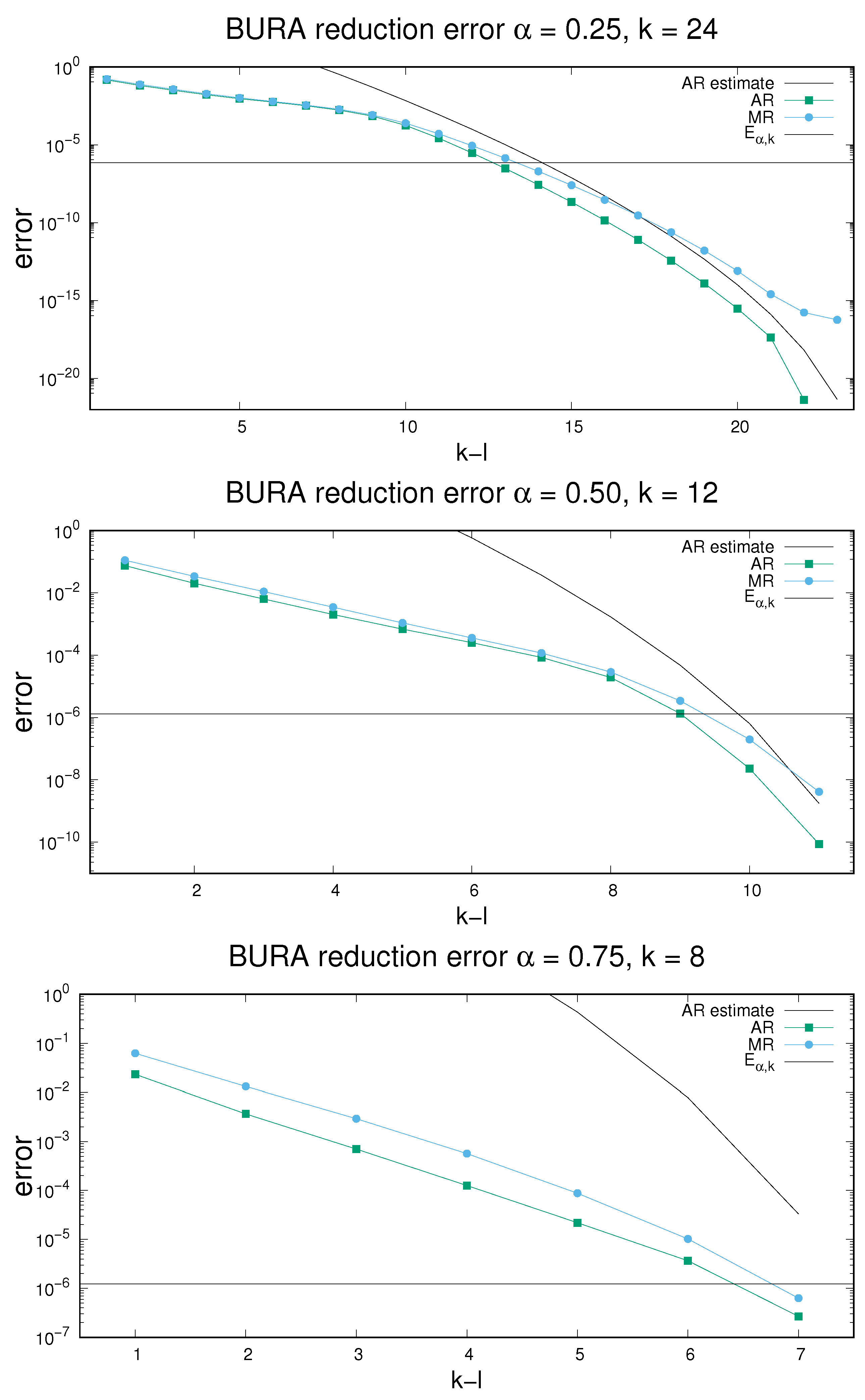
In Figure 6, we compare the BURA reduction errors for $f_2$ to both the theoretical estimate from Theorems 2 and 3 and the corresponding pure non-reduction error $E_{\alpha ,k}$, related to $\ell =0$. All results agree with Theorem 4, as ${∥{\mathbf{u}}_k-{\mathbf{u}}_{k,\ell }^M∥}_2\ge {∥{\mathbf{u}}_k-{\mathbf{u}}_{k,\ell }^A∥}_2$ always holds true. Further, we observe that the difference ${∥{\mathbf{u}}_{k,\ell }^A-{\mathbf{u}}_{k,\ell }^M∥}_2$ decreases when ℓ increases. Finally, the error plots indicate that we can reduce half of the systems ($\ell =12$) for $\alpha =0.25$, one-quarter of the systems ($\ell =3$) for $\alpha =0.5$, and one-eighth of the systems ($\ell =1$) for $\alpha =0.75$, without affecting the order of the overall BURA accuracy.

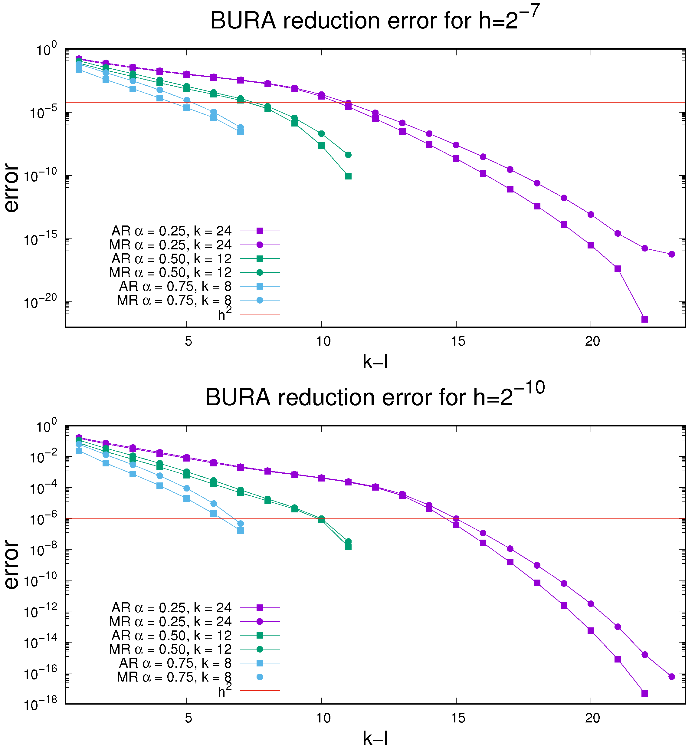
In Figure 7, we compare the BURA reduction errors for $f_2$ with $h^2$—the best order of the discretization error estimate. The idea of this experiment is that whenever the BURA reduction error is below $h^2$, then the total error estimate (11) should be dominated by the error of discretization; thus, the reduction process should again not affect the overall accuracy. We observe that for $h=1/128$∼${10}^{-2}$, we can “safely” reduce 13 systems within both BURA-AR and BURA-MR methods when $\alpha =0.25$. Analogously, we can “safely” reduce 4 systems within both BURA-AR and BURA-MR methods when $\alpha =0.5$, and 3 and 2 systems, respectively, within the BURA-AR and BURA-MR methods, when $\alpha =0.75$. When $h=1/1024$∼${10}^{-3}$, we are within the “optimal” scenario depicted in Table 1 and, as suggested in the last column of the rows corresponding to $h={10}^{-3}$, we witness the possibility of exactly 9 system reductions for $\alpha =0.25$, exactly 2 system reductions for $\alpha =0.5$, and even 1 system reduction for $\alpha =0.75$.

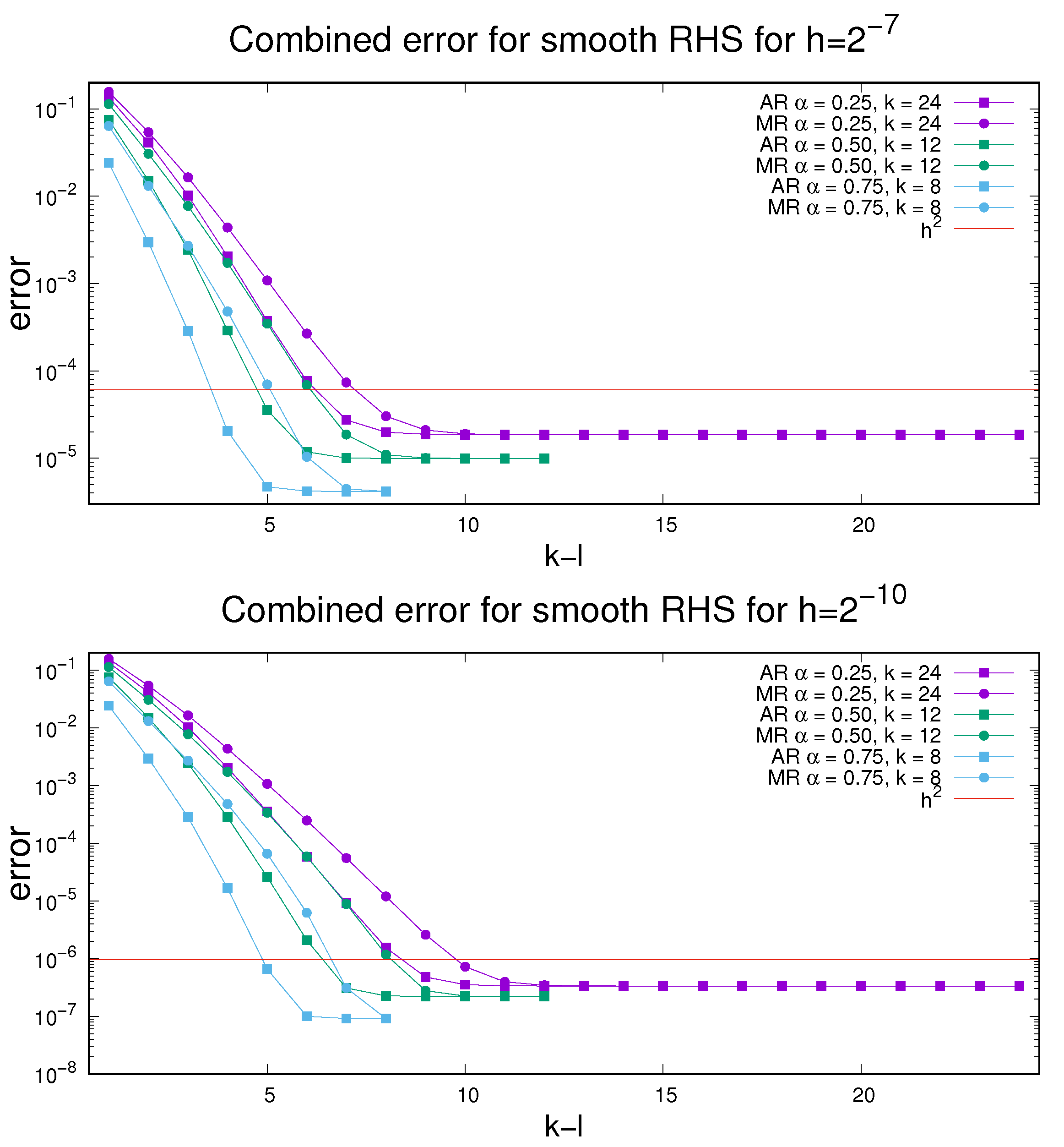
Finally, in Figure 5, we conduct experiments analogous to Figure 6 but using the smooth right-hand side $f_1$ and estimating the total error (11). The level of potential systems reduction is similar to that in the previous experiment. Moreover, we observe the balance between the BURA error and the error of discretization around level $h^2$, especially for finer meshes. This is an indication that the theoretically derived order of discretization of $h^{2\alpha }$ in certain cases (smooth right-hand sides that agree on the boundary with the boundary conditions and give rise to regular solutions) may be too pessimistic and that the upper order estimate of $h^2$, corresponding to classical, non-fractional diffusion, could be achieved, independently of the choice of $\alpha$.

7. Concluding Remarks

The newly obtained results significantly improve the computational efficiency of the BURA method. The fact that practically all other methods for a numerical solution of multidimensional spectral fractional-in-space diffusion problems in arbitrary domains can be viewed as some rational approximation further enhances the advantages of the new BURA-MR and BURA-AR methods. On the other hand, the proposed reduced product/sum approach can be applied to many of the other existing methods, as well. The new theoretical results and the presented proof-of-concept numerical tests open the window for a wide range of real-life applications, including various problems beyond the scalar elliptic case.

The number of auxiliary sparse SPD systems to be solved is applied as a measure of computational efficiency in [9], where the BURA method is introduced. Then, this approach is used in the comparative analysis of various other methods, which can be interpreted as a certain rational approximation of degree k of ${\mathbb{A}}^{-\alpha }$. The theory of the BURA method does not depend on the shape of the computational domain. This also applies to the methods for which the unified approach from [7] is applicable. Based on this, in various papers, one-dimensional numerical tests are considered to be fully representative. In theory, this is correct, but in practice, it is not. The key point in the multidimensional case is that the SPD matrix $\mathbb{A}$ is generally unstructured and large-scale. Thus, the implementation of methods based on rational approximation of degree k naturally involves a certain iterative solver of the related k auxiliary sparse SPD systems. In this spirit is the presented study on the efficient implementation of the BURA method in the case of higher degrees k.

The idea of reducing BURA was firstly discussed in the short paper [19]. Here, we analyzed two alternative methods: the recently proposed BURA-AR together with the new BURA-MR. They are based on the additive and the multiplicative representations of BURA, respectively. Although the two expressions are completely equivalent, the theoretical estimates of the reduced sum BURA-AR and the reduced product BURA-MR, as well as the corresponding numerical results, are different.

Until now, only the additive representation was used in the software implementation of the BURA method for large-scale multidimensional problems. One of the reasons for this is perhaps its better parallelization. Here, we show rather promising results for the multiplicative variant of BURA and related BURA-MR methods. This resumes the discussion of the advantages and disadvantages of both options.

The results of this study contribute to the strengthening of theoretical knowledge and practical skills for a numerical solution of real-life fractional diffusion problems in complex multidimensional domains. At the same time, there are still certain issues related to computational stability that most likely need further understanding, interpretation and treatment.

The development of computationally efficient BURA-AR and BURA-MR methods for reaction-diffusion and time-dependent equations involving fractional-in-space diffusion operators is among the priority topics for further research.

Finally, we observe that under certain assumptions, the computational complexity of the reduced BURA can be improved to $O(NlogN)$.