On a New Modification of the Erdélyi–Kober Fractional Derivative

Abstract

In this paper, we introduce a new Caputo-type modification of the Erdélyi–Kober fractional derivative. We pay attention to how to formulate representations of Erdélyi–Kober fractional integral and derivatives operators. Then, some properties of the new modification and relationships with other Erdélyi–Kober fractional derivatives are derived. In addition, a numerical method is presented to deal with fractional differential equations involving the proposed Caputo-type Erdélyi–Kober fractional derivative. We hope the presented method will be widely applied to simulate such fractional models.

1. Introduction

The fractional calculus theory has recently received considerable attention due to the wide applications of fractional derivative operators in the mathematical modelling of many realistic phenomena that involve non-locality and memory characteristics [1,2,3,4,5,6]. Fractional derivative operators, which are usually defined via fractional integral operators, help to collect useful information about the evolution of the materials and processes involved in the phenomena. In the literature, many fractional derivative operators, such as Riemann–Liouville, Hadamard, Caputo and Erdélyi–Kober fractional operators, have been proposed and implemented. The Riemann–Liouville (R–L) fractional integral operator, which is one of the most used and studied definitions, of order $\alpha >0$ is defined by [1,2,3,4,5]:

$$I_{a+}^{\alpha }f\left(t\right)=\frac{1}{\mathsf{\Gamma }\left(\alpha \right)}{\int }_a^t{(t-\tau )}^{\alpha -1}f\left(\tau \right)d\tau ,t>a.$$

(1)

In light of the above definition, the R–L and Caputo fractional derivative operators of order $\alpha >0$ are defined by [1,2,3,4,5]:

$${}^R{D}_{a+}^{\alpha }f\left(t\right)=D^n{I}_{a+}^{n-\alpha }f\left(t\right)=\frac{1}{\mathsf{\Gamma }(n-\alpha )}\frac{d^n}{d{t}^n}{\int }_a^t{(t-\tau )}^{n-\alpha -1}f\left(\tau \right)d\tau ,t>a,$$

(2)

$${}^C{D}_{a+}^{\alpha }f\left(t\right)=I_{a+}^{n-\alpha }{D}^{n}f\left(t\right)=\frac{1}{\mathsf{\Gamma }(n-\alpha )}{\int }_a^t{(t-\tau )}^{n-\alpha -1}{f}^{\left(n\right)}\left(\tau \right)d\tau ,t>a,$$

(3)

respectively, where $n-1<\alpha \le n$ and $n\in IN$. Details and properties of the above operators can be found in [1,2,3,4,5,6]. In fact, one can easily recognize, for $n-1<\alpha \le n$, $\beta >0$ and $t>a$, the following properties:

$$I_{a+}^{\alpha }{I}_{a+}^{\beta }f\left(t\right)=I_{a+}^{\alpha +\beta }f\left(t\right),$$

(4)

and

$$I_{a+}^{\alpha }{}^C{D}_{a+}^{\alpha }f\left(t\right)=f\left(t\right)-\sum _{k=0}^{n-1}\frac{f^{\left(k\right)}(a+)}{k!}{(t-a)}^k.$$

(5)

The Erdélyi–Kober (E–K) fractional integral operator, $I_{a+;\rho ,\eta }^{\alpha }$, of order $\alpha >0$, which is a modification and extension of the R–L fractional integral operator, is described as [1,5,7]:

$$\left(I_{a+;\rho ,\eta }^{\alpha }f\right)\left(t\right)=\rho \frac{t^{-\rho (\alpha +\eta )}}{\mathsf{\Gamma }\left(\alpha \right)}{\int }_a^t{\tau }^{\rho \eta +\rho -1}{(t^{\rho }-{\tau }^{\rho })}^{\alpha -1}f\left(\tau \right)d\tau ,t>a\ge 0,$$

(6)

with $\rho >0$ and $\eta \in IR$. The E–K fractional integral operator has been used to solve single, double and triple integral equations that have spatial functions of mathematical physics in their kernels. Some applications and properties of the E–K fractional integral operator can be found in [1,5,8,9,10,11,12,13,14,15,16,17,18] and references therein. Based on the fractional integral operator given in Equation (6), the E–K fractional derivative operator, $D_{a+;\rho ,\eta }^{\alpha }$, of order $\alpha >0$, where $n-1<\alpha \le n$, $\rho >0$ and $\eta \in IR$, is defined as: [1,5]

$$\left(D_{a+;\rho ,\eta }^{\alpha }f\right)\left(t\right)=t^{-\rho \eta }{\left(\frac{1}{\rho t^{\rho -1}}\frac{d}{dt}\right)}^n{t}^{\rho (n+\eta )}\left(I_{a+;\rho ,\eta +\alpha }^{n-\alpha }f\right)\left(t\right),t>a\ge 0.$$

(7)

Using the principle that ${\prod }_{j=1}^n\left[\eta +j+\frac{1}{\rho }t\frac{d}{dt}\right](·)=\left[t^{-\rho \eta }{\left(\frac{1}{\rho t^{\rho -1}}\frac{d}{dt}\right)}^n{t}^{\rho (n+\eta )}\right](·)$, an alternative characterization of the E–K fractional derivative operator can be formulated as [19]:

$$\left(D_{a+;\rho ,\eta }^{\alpha }f\right)\left(t\right)=\prod _{j=1}^n\left[\eta +j+\frac{1}{\rho }t\frac{d}{dt}\right]\left(I_{a+;\rho ,\eta +\alpha }^{n-\alpha }f\right)\left(t\right),t>a\ge 0.$$

(8)

In particular, if $\alpha ,\beta >0$, $\rho >0$, $\eta \in IR$ and $t>a\ge 0$, we have the following properties:

$$\left(I_{a+;\rho ,\eta }^{\alpha }{I}_{a+;\rho ,\eta +\alpha }^{\beta }f\right)\left(t\right)=\left(I_{a+;\rho ,\eta }^{\alpha +\beta }f\right)\left(t\right),$$

(9)

and

$$\left(D_{a+;\rho ,\eta }^{\alpha }{I}_{a+;\rho ,\eta }^{\alpha }f\right)\left(t\right)=f\left(t\right),$$

(10)

for “sufficiently good” function f. For more details, properties and characteristics of the E–K fractional integral and derivative operators given in Equations (6) and (7), respectively, the reader is advised to refer to the work presented in [1,5,10,19]. A modification of the E–K fractional derivative operator in the Caputo sense has been introduced in [19]. A brief review of this modification is presented in the next section.

In view of Formula (5), the Caputo fractional derivative has many features similar to integer-order derivatives, and so it is extensively used to model numerous real-life problems in fractional calculus applications. The main objective of this study is to present a Caputo-type adjustment of the E–K fractional derivative, which is somewhat similar to the Caputo fractional derivative given in Equation (3). Then, we discuss some of its properties and relationships with the E–K fractional integral and derivative operators given in Equations (6) and (7). Furthermore, a novel predictor–corrector method for solving Caputo-type E–K fractional differential equations (FDEs) is introduced.

2. Luchko and Trujillo’s Modification

In [19], Luchko and Trujillo define a Caputo-type adjustment of the E–K fractional derivative operator and introduce some of its properties. Let $a=0$, $n-1<\alpha \le n$, $n\in IN$, $\rho >0$ and $\eta \in IR$. The modified E–K fractional derivative operator, ${}_{\ast }{D}_{0+;\rho ,\eta }^{\alpha }$, of order $\alpha$ is defined, according to Ref. [19], as:

$$\left({}_{\ast }{D}_{0;\rho ,\eta }^{\alpha }f\right)\left(t\right)=I_{0;\rho ,\eta +\alpha }^{n-\alpha }\left(\prod _{j=0}^{n-1}\left(1+\eta +j+\frac{1}{\rho }t\frac{d}{dt}\right)f\right)\left(t\right),t>0.$$

(11)

That is,

$$\left({}_{\ast }{D}_{0;\rho ,\eta }^{\alpha }f\right)\left(t\right)=\rho \frac{t^{-\rho (n+\eta )}}{\mathsf{\Gamma }(n-\alpha )}{\int }_0^t{\tau }^{\rho (\eta +\alpha )+\rho -1}{(t^{\rho }-{\tau }^{\rho })}^{n-\alpha -1}\left(\prod _{j=0}^{n-1}\left(1+\eta +j+\frac{1}{\rho }\tau \frac{d}{d\tau }\right)f\right)\left(\tau \right)d\tau .$$

(12)

Define the space of functions $C_{a;\alpha }^n$, where $\alpha \in IR$, $a\ge 0$ and $n\in IN$, to be the set of all functions f that can be expressed in the form $f\left(x\right)=x^p{f}_1\left(x\right)$, $x>a$, with $p>\alpha$ and $f_1\in C^n[a,\infty )$. Accordingly, depending on the previous definitions, we have the following properties and relations.

Theorem 1.

Let $a=0$, $n-1<\alpha \le n$, $n\in IN$, $\rho >0$ and $\eta \in IR$. If $\beta \ge -\rho (\eta +1)$, then the E–K fractional integral operator $I_{0;\rho ,\eta }^{\alpha }$ is a linear map of the space $C_{0;\beta }^0$ into itself. If $\beta \ge -\rho (\eta +1)$ and $f\in C_{0;\beta }^n$, then the E–K fractional derivative $D_{a+;\rho ,\eta }^{\alpha }f\in C_{0;\beta }^0$. Moreover, if $\beta \ge -\rho (\eta +\alpha +1)$ and $f\in C_{0;\beta }^n$, then the Luchko and Trujillo modification of the E–K fractional derivative ${}_{\ast }{D}_{a+;\rho ,\eta }^{\alpha }f\in C_{0;\beta }^0$.

Theorem 2.

Let $a=0$, $n-1<\alpha \le n$, $n\in IN$, $\rho >0$ and $\eta \in IR$.

• If $\beta \ge -\rho (\eta +1)$ and $f\in C_{0;\beta }^0$, then the E–K fractional derivative operator $D_{0;\rho ,\eta }^{\alpha }$ is a left-inverse of the E–K fractional integral operator $I_{0;\rho ,\eta }^{\alpha }$.
• If $\beta \ge -\rho (\eta +\alpha +1)$ and $f\in C_{0;\beta }^n$, then the following relationship between the E–K fractional integral and the Luchko and Trujillo’s modification of order α holds.

  $$\left(I_{0;\rho ,\eta }^{\alpha }{}_{\ast }{D}_{0;\rho ,\eta }^{\alpha }f\right)\left(t\right)=f\left(t\right)-\sum _{k=0}^{n-1}{p}_k{t}^{-\rho (\eta +k+1)},$$

  (13)

  where

  $$p_k=\underset{t⟶0}{\lim }{t}^{\rho (\eta +k+1)}\prod _{i=k+1}^{n-1}\left(\eta +i+1+\frac{1}{\rho }t\frac{d}{dt}\right)f\left(t\right).$$

  (14)
• If $f\in C_{0;\beta }^0$, where $\beta >-\rho (\eta +1)$, then the following inverse property holds:

  $$\left({}_{\ast }{D}_{0;\rho ,\eta }^{\alpha }{I}_{0;\rho ,\eta }^{\alpha }f\right)\left(t\right)=f\left(t\right).$$

  (15)

The proof of Theorems 1 and 2 is given in [19]. The main advantage of Luchko and Trujillo’s modification is that the constants $p_k$, $k=0,1,\cdots ,n-1$, given in Equation (14), are based on the integer-order derivatives of the function f and are not conditioned by the initial values of the E–K fractional integrals at $t=0$.

3. The New Modification

In this section, we introduce and provide some characteristics of a new Caputo-type adjustment of the E–K fractional derivative. Initially, we investigate a useful connection between the E–K fractional integral operator, $I_{a+;\rho ,\eta }^{\alpha }$, given in (6) and the R–L fractional integral operator, $I_a^{\alpha }$, given in Equation (1).

Theorem 3.

Let $\alpha >0$, $\rho >0$ and $\eta \in IR$. Then,

$$\left(I_{a+;\rho ,\eta }^{\alpha }f\right)\left(t\right)=\left(x^{-\alpha -\eta }{I}_{a^{\rho }}^{\alpha }\left(x^{\eta }f\left(x^{1/\rho }\right)\right)\right){|}_{x=t^{\rho }},t>a\ge 0.$$

(16)

Proof. 

Applying the change of variables $z={\tau }^{\rho }$ to the E–K fractional integral formula given in Equation (6) yields:

$$\begin{array}{ccc}\left(I_{a+;\rho ,\eta }^{\alpha }f\right)\left(t\right)\hfill & =\hfill & \frac{t^{-\rho (\alpha +\eta )}}{\mathsf{\Gamma }\left(\alpha \right)}{\int }_{a^{\rho }}^{t^{\rho }}{(t^{\rho }-z)}^{\alpha -1}{z}^{\eta }f\left(z^{1/\rho }\right)dz.\hfill \\ \hfill & =\hfill & \left(\frac{x^{-(\alpha +\eta )}}{\mathsf{\Gamma }\left(\alpha \right)}{\int }_{a^{\rho }}^x{(x-z)}^{\alpha -1}{z}^{\eta }f\left(z^{1/\rho }\right)dz\right){|}_{x=t^{\rho }}.\hfill \end{array}$$

(17)

Comparing the above integral with the R–L fractional integral given in Equation (1), the relation (16) can be, thus, derived. □

Indeed, if $n-1<\alpha \le n$ and $n\in IN$, we observe that the R–L fractional operator given in Equation (2) can be produced from the fractional integral operator presented in Equation (1) by replacing the operator $I_{a+}^{\alpha }$ with the composite operators $D^n{I}_{a+}^{n-\alpha }$. Now, if we replace the term $x^{-\alpha -\eta }$ by $x^{-\eta }$, the operator $I_{a^{\rho }}^{\alpha }$ by the composite operators $D^n{I}_{a^{\rho }}^{n-\alpha }$ and the term $x^{\eta }$ by $x^{\eta +\alpha }$ in the right-hand side of Formula (16), we get:

$$\begin{array}{c}\left(x^{-\eta }{D}^n{I}_{a^{\rho }}^{n-\alpha }\left(x^{\eta +\alpha }f\left(x^{1/\rho }\right)\right)\right){|}_{x=t^{\rho }}=\left(\frac{x^{-\eta }}{\mathsf{\Gamma }(n-\alpha )}{D}^n{\int }_{a^{\rho }}^x{(x-z)}^{n-\alpha -1}{z}^{\eta +\alpha }f\left(z^{1/\rho }\right)dz\right){|}_{x=t^{\rho }},\hfill \\ =\left(\rho \frac{x^{-\eta }}{\mathsf{\Gamma }(n-\alpha )}{D}^n{\int }_a^{x^{1/\rho }}{(x-{\tau }^{\rho })}^{n-\alpha -1}{\tau }^{\rho (\eta +\alpha )+\rho -1}f\left(\tau \right)d\tau \right){|}_{x=t^{\rho }},\hfill \end{array}$$

(18)

using the change of variables $\tau =z^{1/\rho }$, where $n-1<\alpha \le n$, $n\in IN$, $\rho >0$ and $\eta \in IR$. Following the rule that $\left(D^{n}f\left(x\right)\right){|}_{x=t^{\rho }}={\left(\frac{1}{\rho t^{\rho -1}}D\right)}^n\left(f\left(t^{\rho }\right)\right)$, we obtain:

$$\begin{array}{c}\left(x^{-\eta }{D}^n{I}_{a^{\rho }}^{n-\alpha }\left(x^{\eta +\alpha }f\left(x^{1/\rho }\right)\right)\right){|}_{x=t^{\rho }}=\rho \frac{t^{-\rho \eta }}{\mathsf{\Gamma }(n-\alpha )}{\left(\frac{1}{\rho t^{\rho -1}}D\right)}^n{\int }_a^t{(t^{\rho }-{\tau }^{\rho })}^{n-\alpha -1}{\tau }^{\rho (\eta +\alpha )+\rho -1}f\left(\tau \right)d\tau ,\hfill \\ =t^{-\rho \eta }{\left(\frac{1}{\rho t^{\rho -1}}\frac{d}{dt}\right)}^n{t}^{\rho (n+\eta )}\left(I_{a+;\rho ,\eta +\alpha }^{n-\alpha }f\right)\left(t\right).\hfill \end{array}$$

(19)

Consequently, the E–K fractional derivative operator given in Equation (7) can be reformulated as:

$$\left(D_{a+;\rho ,\eta }^{\alpha }f\right)\left(t\right)=\left(x^{-\eta }{D}^n{I}_{a^{\rho }}^{n-\alpha }\left(x^{\eta +\alpha }f\left(x^{1/\rho }\right)\right)\right){|}_{x=t^{\rho }},t>a\ge 0.$$

(20)

Now, in a similar manner, the suggested Caputo-type modification of the E–K fractional derivative operator, $D_{a+;\rho ,\eta }^{\alpha }$, can be defined by replacing the term $x^{-\alpha -\eta }$ by $x^{-\eta }$, the operator $I_{a^{\rho }}^{\alpha }$ by the composite operators $I_{a^{\rho }}^{n-\alpha }{D}^n$ and the term $x^{\eta }$ by $x^{\eta +\alpha }$ in the right-hand side of Formula (16) (i.e., interchanging the order of the operators $D^n$ and $I_{a^{\rho }}^{n-\alpha }$ in Formula (20)). So, using the conceptual relationship:

$$\left(D_{a+;\rho ,\eta }^{\alpha }f\right)\left(t\right)=\left(x^{-\eta }{I}_{a^{\rho }}^{n-\alpha }{D}^n\left(x^{\eta +\alpha }f\left(x^{1/\rho }\right)\right)\right){|}_{x=t^{\rho }},t>a\ge 0,$$

(21)

we get

$$\begin{array}{ccc}\left(D_{a+;\rho ,\eta }^{\alpha }f\right)\left(t\right)\hfill & =\hfill & \left(\frac{x^{-\eta }}{\mathsf{\Gamma }(n-\alpha )}{\int }_{a^{\rho }}^x{(x-z)}^{n-\alpha -1}{D}^n\left(z^{\eta +\alpha }f\left(z^{1/\rho }\right)\right)dz\right){|}_{x=t^{\rho }},\hfill \\ \hfill & =\hfill & \left(\frac{\rho x^{-\eta }}{\mathsf{\Gamma }(n-\alpha )}{\int }_a^{x^{1/\rho }}{\tau }^{\rho -1}{(x-{\tau }^{\rho })}^{n-\alpha -1}{\left(\frac{1}{\rho {\tau }^{\rho -1}}D\right)}^n\left({\tau }^{\rho (\eta +\alpha )}f\left(\tau \right)\right)d\tau \right){|}_{x=t^{\rho }},\hfill \end{array}$$

(22)

where $\tau =z^{1/\rho }$, which suggests the following characterization.

Definition 1.

Let $n-1<\alpha \le n$, $n\in IN$, $\rho >0$ and $\eta \in IR$. The new Caputo-type modification of the E–K fractional derivative operator, $D_{a+;\rho ,\eta }^{\alpha }$, of order α is defined as:

$$\left(D_{a+;\rho ,\eta }^{\alpha }f\right)\left(t\right)=\rho \frac{t^{-\rho \eta }}{\mathsf{\Gamma }(n-\alpha )}{\int }_a^t{\tau }^{\rho -1}{(t^{\rho }-{\tau }^{\rho })}^{n-\alpha -1}{\left(\frac{1}{\rho {\tau }^{\rho -1}}D\right)}^n{\tau }^{\rho (\eta +\alpha )}f\left(\tau \right)d\tau ,$$

(23)

where $t>a\ge 0$.

Remark 1.

The new Caputo-type adjustment of the E–K fractional derivative operator, using (6) and (22), can be reformulated as, where $n-1<\alpha \le n$, $n\in IN$, $\rho >0$ and $\eta \in IR$,

$$\left(D_{a+;\rho ,\eta }^{\alpha }f\right)\left(t\right)=t^{\rho n}{I}_{a+;\rho ,\eta +\alpha }^{n-\alpha }{t}^{-\rho (\eta +\alpha )}{\left(\frac{1}{\rho t^{\rho -1}}D\right)}^n{t}^{\rho (\eta +\alpha )}f\left(t\right),t>a\ge 0.$$

(24)

Theorem 4.

Let $a\ge 0$, $n-1<\alpha \le n$, $n\in IN$, $\rho >0$, $\eta \in IR$ and $f\in C_{a;\beta }^n$. Then, $\left(D_{a+;\rho ,\eta }^{\alpha }f\right)\left(t\right)\in C_{a;\beta }^0$ if $\beta \ge -\rho (\eta +\alpha -n+1)$.

Proof. 

Assume that $f\left(t\right)=t^p{f}_1\left(t\right)$, where $f_1\in C^n[a,\infty )$ and $p>\beta$, then, using simple calculations, we can obtain that

$$t^{-\rho (\eta +\alpha )}{\left(\frac{1}{\rho t^{\rho -1}}D\right)}^n{t}^{\rho (\eta +\alpha )}f\left(t\right)=\sum _{k=0}^{n-1}{c}_k{t}^{p-\rho n+k}{f}_1^{\left(k\right)}\left(t\right),$$

(25)

for some constants $c_0$, $c_1$, ⋯, $c_{n-1}$. Now, from Theorem 1, we can observe that the E–K fractional integral operator $I_{a+;\rho ,\eta +\alpha }^{n-\alpha }$ is a linear map of the space $C_{a;\gamma }^0$ into itself when $\gamma \ge -\rho (\eta +\alpha +1)$. Therefore, using the relation (24), we can conclude that $t^{-\rho n}·\left(D_{a+;\rho ,\eta }^{\alpha }f\right)\left(t\right)\in C_{a;\beta -\rho n}^0$ if $\beta -\rho n\ge -\rho (\eta +\alpha +1)$, and so $\left(D_{a+;\rho ,\eta }^{\alpha }f\right)\left(t\right)\in C_{a;\beta }^0$ if $\beta \ge -\rho (\eta +\alpha +1)+\rho n$. □

We can easily observe that in the case of $\rho =1$ our modification $\left(D_{a+;\rho ,\eta }^{\alpha }f\right)\left(t\right)$, according to Definition 1, reduces to $t^{-\eta }{}^C{D}_{a+}^{\alpha }{t}^{\eta +\alpha }f\left(t\right)$, where ${}^C{D}_{a+}^{\alpha }$ is the Caputo fractional derivative operator presented in (3). Next, we investigate the main property of our new modification.

Theorem 5.

Let $a\ge 0$, $n-1<\alpha \le n$, $n\in IN$, $\rho >0$, $\eta \in IR$, $\beta \ge -\rho (\eta +\alpha -n+1)$ and $f\in C_{a;\beta }^n$. Then the following relationship between the E–K fractional integral, introduced in Equation (6), and our adjustment of the E–K fractional derivative holds:

$$\left(I_{a+;\rho ,\eta }^{\alpha }{D}_{a+;\rho ,\eta }^{\alpha }f\right)\left(t\right)=f\left(t\right)-t^{-\rho (\alpha +\eta )}\sum _{k=0}^{n-1}\frac{1}{k!}{\left(x^{\eta +\alpha }f\left(x^{1/\rho }\right)\right)}^{\left(k\right)}{|}_{x=a^{\rho }}·{(t^{\rho }-a^{\rho })}^k.$$

(26)

Proof. 

Firstly, we have $\left(D_{a+;\rho ,\eta }^{\alpha }f\right)\left(t\right)\in C_{a;\beta }^0$ and $\beta \ge -\rho (\eta +1)$ if $\beta \ge -\rho (\eta +\alpha -n+1)$, and so $\left(I_{a+;\rho ,\eta }^{\alpha }{D}_{a+;\rho ,\eta }^{\alpha }f\right)\left(t\right)\in C_{a;\beta }^0$. According to the conceptual relationships given in Formulas (16) and (21), the following relation holds:

$$\begin{array}{ccc}\left(I_{a+;\rho ,\eta }^{\alpha }{D}_{a+;\rho ,\eta }^{\alpha }f\right)\left(t\right)\hfill & =\hfill & \left(x^{-\alpha -\eta }{I}_{a^{\rho }}^{\alpha }\left\{x^{\eta }\left(D_{a+;\rho ,\eta }^{\alpha }f\right)\left(x^{1/\rho }\right)\right\}\right){|}_{x=t^{\rho }},\hfill \\ \hfill & =\hfill & \left(x^{-\alpha -\eta }{I}_{a^{\rho }}^{\alpha }\left\{x^{\eta }\left(x^{-\eta }{I}_{a^{\rho }}^{n-\alpha }{D}^n\left(x^{\eta +\alpha }f\left(x^{1/\rho }\right)\right)\right)\right\}\right){|}_{x=t^{\rho }}.\hfill \end{array}$$

(27)

Following property (4), we get

$$\left(I_{a+;\rho ,\eta }^{\alpha }{D}_{a+;\rho ,\eta }^{\alpha }f\right)\left(t\right)=\left(x^{-\alpha -\eta }{I}_{a^{\rho }}^n{D}^n\left(x^{\eta +\alpha }f\left(x^{1/\rho }\right)\right)\right){|}_{x=t^{\rho }}.$$

(28)

Using Theorem 2 and the fact that $I_a^n{D}^{n}f\left(x\right)=f\left(x\right)-{\displaystyle \sum _{k=0}^{n-1}}\frac{f^{\left(k\right)}\left(a\right)}{k!}{(x-a)}^k$, we obtain

$$\begin{array}{c}\left(I_{a+;\rho ,\eta }^{\alpha }{D}_{a+;\rho ,\eta }^{\alpha }f\right)\left(t\right)=\left(x^{-\alpha -\eta }\left\{x^{\eta +\alpha }f\left(x^{1/\rho }\right)-{\displaystyle \sum _{k=0}^{n-1}}\frac{1}{k!}{\left(x^{\eta +\alpha }f\left(x^{1/\rho }\right)\right)}^{\left(k\right)}{|}_{x=a^{\rho }}·{(x-a^{\rho })}^k\right\}\right){|}_{x=t^{\rho }},\hfill \\ =f\left(t\right)-t^{-\rho (\alpha +\eta )}{\displaystyle \sum _{k=0}^{n-1}}\frac{1}{k!}{g}^{\left(k\right)}\left(a^{\rho }\right)·{(t^{\rho }-a^{\rho })}^k,\hfill \end{array}$$

(29)

where $g\left(x\right)=x^{\eta +\alpha }f\left(x^{1/\rho }\right)$. □

Remark 2.

In particular, given $0<\alpha \le 1$, the relation (26) reduces to

$$\left(I_{a+;\rho ,\eta }^{\alpha }{D}_{a+;\rho ,\eta }^{\alpha }f\right)\left(t\right)=f\left(t\right)-a^{\rho (\alpha +\eta )}f\left(a\right)·t^{-\rho (\alpha +\eta )}.$$

(30)

Remark 3.

If $a=0$, $\rho >0$, $\eta \in IR$ and $0<\alpha <1$ then the Luchko and Trujillo’s modification and our adjustment of the E–K fractional derivative given in Formulas (12) and (23), when $t>0$, reduce to:

$$\left({}_{\ast }{D}_{0;\rho ,\eta }^{\alpha }f\right)\left(t\right)=\frac{t^{-\rho (\eta +1)}}{\mathsf{\Gamma }(1-\alpha )}{\int }_0^t{\tau }^{\rho (\eta +\alpha +1)-1}{(t^{\rho }-{\tau }^{\rho })}^{-\alpha }\left\{\rho (\eta +1)f\left(\tau \right)+\tau f^{\prime }\left(\tau \right)\right\}d\tau ,$$

(31)

and

$$\left(D_{0;\rho ,\eta }^{\alpha }f\right)\left(t\right)=\frac{t^{-\rho \eta }}{\mathsf{\Gamma }(1-\alpha )}{\int }_0^t{\tau }^{\rho (\eta +\alpha )-1}{(t^{\rho }-{\tau }^{\rho })}^{-\alpha }\left\{\rho (\eta +\alpha )f\left(\tau \right)+\tau f^{\prime }\left(\tau \right)\right\}d\tau ,$$

(32)

respectively. Comparing (31) with (32), in general, we can conclude that they are not identical. For example, if we take $f\left(t\right)=1$ with the parameters $a=0$, $\rho >0$, $0<\alpha <1$ and $\eta =-\alpha$ then, using Equations (31) and (32), we obtain $\left({}_{\ast }{D}_{0;\rho ,\eta }^{\alpha }f\right)\left(t\right)=\frac{1}{\mathsf{\Gamma }(1-\alpha )}$ while $\left(D_{0;\rho ,\eta }^{\alpha }f\right)\left(t\right)=0$. Therefore, the Luchko and Trujillo’s modification and our adjustment of the E–K fractional derivative are not equivalent.

Remark 4.

In particular, if $0<\alpha <1$, $a\ge 0$, $\rho >0$, $\eta \in IR$, $\beta \ge -\rho (\eta +\alpha )$, $f\in C_{a;\beta }^0$ and $g\left(t\right)=\left(I_{a+;\rho ,\eta }^{\alpha }f\right)\left(t\right)$ then, form the relation (10) and using Theorem 5, we get:

$$\left(D_{a+;\rho ,\eta }^{\alpha }g\right)\left(t\right)=D_{a+;\rho ,\eta }^{\alpha }\left\{g\left(t\right)-a^{\rho (\alpha +\eta )}g\left(a\right)·t^{-\rho (\alpha +\eta )}\right\}.$$

(33)

So, since $g\left(a\right)=0$, we obtain:

$$\left(D_{a+;\rho ,\eta }^{\alpha }{I}_{a+;\rho ,\eta }^{\alpha }f\right)\left(t\right)=\left(D_{a+;\rho ,\eta }^{\alpha }{I}_{a+;\rho ,\eta }^{\alpha }f\right)\left(t\right)=f\left(t\right).$$

(34)

Remark 5.

If we simplify the term ${\left(x^{\eta +\alpha }f\left(x^{1/\rho }\right)\right)}^{\left(k\right)}{|}_{x=a^{\rho }}$ in the relation (26), we can show that $\left(I_{a+;\rho ,\eta }^{\alpha }{D}_{a+;\rho ,\eta }^{\alpha }f\right)\left(t\right)$ depends on integer derivatives of the function f at a, which is the same case in the relation (5).

Remark 6.

If we take $\eta =-\alpha$ and $\rho =1$ then the relation (26) reduces to:

$$\left(I_{a+;1,-\alpha }^{\alpha }{D}_{a+;1,-\alpha }^{\alpha }f\right)\left(t\right)=f\left(t\right)-\sum _{k=0}^{n-1}\frac{1}{k!}{f}^{\left(k\right)}\left(a\right)·{(t-a)}^k=\left(I_{a+}^{\alpha }{}^C{D}_{a+}^{\alpha }f\right)\left(t\right).$$

(35)

Hence, the relation between our modification and the E–K fractional integral, given in Equation (26), can be considered as a generalization of the relation between the R–L integral and the Caputo derivative, given in Equation (5).

Note that the property (10) holds if $f\in C_{a;\beta }^0$, where $\beta \ge -\rho (\eta +1)$, and that $\beta \ge -\rho (\eta +1)$ if $\beta \ge -\rho (\eta +\alpha -n+1)$. Applying now the E–K fractional derivative operator, $D_{a+;\rho ,\eta }^{\alpha }$, to both sides of the relation (26), using the property (10), we gain the following result.

Theorem 6.

Let $a\ge 0$, $n-1<\alpha \le n$, $n\in IN$, $\rho >0$, $\eta \in IR$, $\beta \ge -\rho (\eta +\alpha -n+1)$ and $f\in C_{a;\beta }^n$. Then the below relationship between our adjustment of the E–K fractional derivative given in Definition 1 and the E–K fractional derivative given in Equation (7) holds:

$$\left(D_{a+;\rho ,\eta }^{\alpha }f\right)\left(t\right)=D_{a+;\rho ,\eta }^{\alpha }\left\{f\left(t\right)-t^{-\rho (\alpha +\eta )}\sum _{k=0}^{n-1}\frac{1}{k!}{\left(x^{\eta +\alpha }f\left(x^{1/\rho }\right)\right)}^{\left(k\right)}{|}_{x=a^{\rho }}·{(t^{\rho }-a^{\rho })}^k\right\}.$$

(36)

Remark 7.

If we have $\left[\frac{d^k}{d{x}^k}\left(x^{\eta +\alpha }f\left(x^{1/\rho }\right)\right)\right]{|}_{x=a^{\rho }}=0$, for all $k=0,1,\cdots n-1$, then, in accordance with Theorem 6, the new adjustment of the E–K fractional derivative matches the E–K fractional derivative given in Equation (7) (i.e., $\left(D_{a+;\rho ,\eta }^{\alpha }f\right)\left(t\right)=\left(D_{a+;\rho ,\eta }^{\alpha }f\right)\left(t\right)$ ).

Next, we give our new adjustment of the E–K fractional derivative for the function $f\left(t\right)=t^{-\rho (\eta +\alpha )}{(t^{\rho }-a^{\rho })}^v$. Let $n-1<\alpha \le n$, $n\in IN$, $\rho >0$, $\eta \in IR$, $\upsilon >n-1$ and $\upsilon \notin IN$. Then, using the relation (21), we have, for $t>a$,

$$\begin{array}{c}{D}_{a+;\rho ,\eta }^{\alpha }\left\{t^{-\rho (\eta +\alpha )}{(t^{\rho }-a^{\rho })}^v\right\}=\left\{x^{-\eta }{I}_{a^{\rho }}^{n-\alpha }{D}^n{\left(x-a^{\rho }\right)}^{\upsilon }\right\}{|}_{x=t^{\rho }},\hfill \\ =\upsilon (\upsilon -1)\cdots (\upsilon -n+1)\left\{x^{-\eta }{I}_{a^{\rho }}^{n-\alpha }{\left(x-a^{\rho }\right)}^{\upsilon -n}\right\}{|}_{x=t^{\rho }}.\hfill \end{array}$$

(37)

Using the properties of the R–L integral operator, we get:

$$I_{a^{\rho }}^{n-\alpha }{\left(x-a^{\rho }\right)}^{\upsilon -n}=\frac{\mathsf{\Gamma }(\upsilon -n+1)}{\mathsf{\Gamma }(\upsilon -\alpha +1)}{\left(x-a^{\rho }\right)}^{\upsilon -\alpha }.$$

(38)

Substituting (38) into (37), we obtain the result:

$$D_{a+;\rho ,\eta }^{\alpha }\left\{t^{-\rho (\eta +\alpha )}{(t^{\rho }-a^{\rho })}^v\right\}=\frac{\mathsf{\Gamma }(\upsilon +1)}{\mathsf{\Gamma }(\upsilon -\alpha +1)}{t}^{-\rho \eta }{\left(t^{\rho }-a^{\rho }\right)}^{\upsilon -\alpha }.$$

(39)

The last problem that we consider here is to verify that our adjustment of the E–K fractional derivative operator $D_{a+;\rho ,\eta }^{\alpha }$ is a left inverse to the E–K fractional integral operator $I_{a+;\rho ,\eta }^{\alpha }$.

Theorem 7.

Let $a\ge 0$, $n-1<\alpha \le n$, $n\in IN$, $\rho >0$, $\eta \in IR$, $\beta \ge -\rho (\eta +\alpha -n+1)$ and $f\in C_{a;\beta }^0$. Then the following rule holds:

$$\left(D_{a+;\rho ,\eta }^{\alpha }{I}_{a+;\rho ,\eta }^{\alpha }f\right)\left(t\right)=f\left(t\right).$$

(40)

Proof. 

Define the function h as $h\left(x\right)=\left(I_{a+;\rho ,\eta }^{\alpha }f\right)\left(x\right)$, then, using Theorem 3, we have:

$$x^{\alpha +\eta }h\left(x^{1/\rho }\right)=I_{a^{\rho }}^{\alpha }\left\{x^{\eta }f\left(x^{1/\rho }\right)\right\}.$$

(41)

Following the R–L integral operator properties, for $k=0,1,\cdots n-1$, we obtain:

$$\begin{array}{ccc}\frac{d^k}{d{x}^k}\left(x^{\alpha +\eta }h\left(x^{1/\rho }\right)\right)\hfill & =\hfill & D^k{I}_{a^{\rho }}^{\alpha }\left\{x^{\eta }f\left(x^{1/\rho }\right)\right\},\hfill \\ \hfill & =\hfill & D^k{I}_{a^{\rho }}^k{I}_{a^{\rho }}^{\alpha -k}\left\{x^{\eta }f\left(x^{1/\rho }\right)\right\},\hfill \\ \hfill & =\hfill & I_{a^{\rho }}^{\alpha -k}\left\{x^{\eta }f\left(x^{1/\rho }\right)\right\}.\hfill \end{array}$$

(42)

However, using the relation (16), we have $\left(I_{a^{\rho }}^{\alpha -k}\left\{x^{\eta }f\left(x^{1/\rho }\right)\right\}\right){|}_{x=t^{\rho }}=t^{\rho (\alpha +\eta -k)}\left(I_{a+;\rho ,\eta }^{\alpha -k}f\right)\left(t\right)$. Furthermore, because $I_{a+;\rho ,\eta }^{\alpha -k}f\in C_{a;\beta }^0$ and $\rho (\eta +\alpha -k)\ge \rho (\eta +\alpha -n+1)$, we can simply conclude that $\left(I_{a^{\rho }}^{\alpha -k}\left\{x^{\eta }f\left(x^{1/\rho }\right)\right\}\right){|}_{x=t^{\rho }}\in C_{a;0}^0$. Thus,

$$\left[\frac{d^k}{d{x}^k}\left(x^{\alpha +\eta }h\left(x^{1/\rho }\right)\right)\right]{|}_{x=a^{\rho }}=0.$$

(43)

Therefore, using Theorem 6, we obtain: $\left(D_{a+;\rho ,\eta }^{\alpha }h\right)\left(t\right)=\left(D_{a+;\rho ,\eta }^{\alpha }h\right)\left(t\right)$, and so,

$$\left(D_{a+;\rho ,\eta }^{\alpha }{I}_{a+;\rho ,\eta }^{\alpha }f\right)\left(t\right)=\left(D_{a+;\rho ,\eta }^{\alpha }{I}_{a+;\rho ,\eta }^{\alpha }f\right)\left(t\right)=f\left(t\right).$$

(44)

□

Remark 8.

By comparing the conceptual relationships presented in Equations (20) and (21), we can notice that our adjustment of the E–K fractional derivative $D_{a+;\rho ,\eta }^{\alpha }$ has reformulated the E–K fractional derivative $D_{a+;\rho ,\eta }^{\alpha }$, given in (7), by switching the arrangement of the integer-order derivative operator $D^n$ with the fractional integral operator $I_{a^{\rho }}^{n-\alpha }$.

Integral equations with E–K fractional operators are often applicable in the theories of neutron transport, radiative transfer, kinetic energy of gases and in the traffic theory. Therefore, in view of the studied relationships and properties, we hope that the presented Caputo-type modification of the E–K fractional derivative can be more successfully applied in various fields of the above mentioned research and modelling.

4. Numerical Simulation of Caputo-Type E–K FDEs

In this section, we suggest a numerical method based on the predictor–corrector methods [20,21,22] to solve numerically fractional differential equation involving the new Caputo-type adjustment of the E–K fractional derivative. Novel fractional models have been considered and numerical simulation results for such models using our algorithm have been provided. For this section purpose, we consider the Caputo-type E–K FDE

$$\left(D_{a+;\rho ,\eta }^{\alpha }y\right)\left(t\right)=F(t,y\left(t\right)),t>a\ge 0,$$

(45)

where $n-1<\alpha \le n$, $n\in IN$, $\rho >0$, $\eta \in IR$ and $D_{a+;\rho ,\eta }^{\alpha }$ is the new Caputo-type adjustment of the E–K fractional derivative explained in Definition 1, with the initial conditions

$$y^{\left(k\right)}\left(a\right)=y_a^k,k=0,1,\cdots ,n-1.$$

(46)

In the first place, let $\beta \ge -\rho (\eta +\alpha -n+1)$ and $y\in C_{a;\beta }^n$ then, by using Theorem 5, the IVP consisting of the Caputo-type E–K FDE (45) and the initial conditions given in (46) is exactly equivalent to the following integral equation

$$y\left(t\right)=x\left(t\right)+\rho \frac{t^{-\rho (\alpha +\eta )}}{\mathsf{\Gamma }\left(\alpha \right)}{\int }_a^t{\tau }^{\rho \eta +\rho -1}{(t^{\rho }-{\tau }^{\rho })}^{\alpha -1}F(\tau ,y\left(\tau \right))d\tau ,$$

(47)

where

$$x\left(t\right)=t^{-\rho (\alpha +\eta )}\sum _{k=0}^{n-1}\frac{1}{k!}{\left(x^{\eta +\alpha }y\left(x^{1/\rho }\right)\right)}^{\left(k\right)}{|}_{x=a^{\rho }}·{(t^{\rho }-a^{\rho })}^k.$$

(48)

Here the function F and the constants $\eta$ and $\rho$ are assumed so that a unique solution to the IVP (45) and (46) exits in the interval $[a,b]$. Define the nonuniform gird in the interval $[a,b]$ with $N+1$ non-equispaced nodes $t_k$, $k=0,1,\cdots N$, as

$$\left\{\begin{array}{ccc}{t}_0\hfill & =\hfill & a,\hfill \\ t_{k+1}\hfill & =\hfill & {(t_k^{\rho }+h)}^{1/\rho },k=0,1,\cdots ,N-1,\hfill \end{array}\right.$$

(49)

such that $h=\frac{b^{\rho }-a^{\rho }}{N}$. Next, we will numerically calculate the approximations $y_k$, $k=0,1,\cdots ,N$ for the IVP (45) and (46) solution. The key step of our algorithm, assuming we have actually computed the approximations ${\{y_j\approx y\left(t_j\right)\}}_{j=1}^k$, is that we need to provide the approximation $y_{k+1}\approx y\left(t_{k+1}\right)$ via the equation:

$$y\left(t_{k+1}\right)=x\left(t_{k+1}\right)+\rho \frac{t_{k+1}^{-\rho (\alpha +\eta )}}{\mathsf{\Gamma }\left(\alpha \right)}{\int }_a^{t_{k+1}}{\tau }^{\rho -1}{(t_{k+1}^{\rho }-{\tau }^{\rho })}^{\alpha -1}{\tau }^{\rho \eta }F(\tau ,y\left(\tau \right))d\tau .$$

(50)

Consequently, by following the derivation of the adaptive predictor–corrector algorithm presented in [22], our predictor–corrector algorithm, to provide the numerical approximation $y_{k+1}\approx y\left(t_{k+1}\right)$ for the IVP (45) and (46), can be described by the rule:

$$y_{k+1}\approx x\left(t_{k+1}\right)+t_{k+1}^{-\rho (\alpha +\eta )}\frac{h^{\alpha }}{\mathsf{\Gamma }(\alpha +2)}\left\{\sum _{j=0}^k{c}_{j,k+1}G(t_j,y_j)+G(t_{k+1},y_{k+1}^p)\right\},$$

(51)

such that the predicted value $y_{k+1}^P\approx y^P\left(t_{k+1}\right)$ can be found out using the formula:

$$y^P\left(t_{k+1}\right)\approx x\left(t_{k+1}\right)+\frac{h^{\alpha }}{\mathsf{\Gamma }(\alpha +1)}{t}_{k+1}^{-\rho (\alpha +\eta )}\sum _{j=0}^k\left[{(k+1-j)}^{\alpha }-{(k-j)}^{\alpha }\right]G(t_j,y\left(t_j\right)),$$

(52)

with the weights $c_{j,k+1}$ described as:

$$c_{j,k+1}=\left\{\begin{array}{ccc}{k}^{\alpha +1}-(k-\alpha ){(k+1)}^{\alpha }\hfill & \hfill & ifj=0,\hfill \\ {(k-j)}^{\alpha +1}-2{(k-j+1)}^{\alpha +1}+{(k-j+2)}^{\alpha +1}\hfill & \hfill & if1\le j\le k,\hfill \end{array}\right.$$

(53)

and $G(t,y\left(t\right))=t^{\rho \eta }F(t,y\left(t\right))$. It is easy to notice, for implementation purposes, that our algorithm does not depend on the choice of the value of the parameters $\alpha$, $\rho$ and $\eta$ and so, its features are similar to those of the classical Adams–Bashforth–Moulton method. Hence, our algorithm works successfully with respect to the numerical stability of the provided approximations. Now, we consider Caputo-type E–K fractional models as test problems to exhibit the effectiveness of the proposed numerical method.

Illustrative Example 1. Our first example deals with the Caputo-type E–K initial value problem.

$$\left(D_{0+;\rho ,\eta }^{\alpha }y\right)\left(t\right)=\frac{2}{\mathsf{\Gamma }(3-\alpha )}{t}^{\rho (2-\alpha -\eta )}-y^2+t^{2\rho (2-\alpha -\eta )},y\left(0\right)=0,$$

(54)

where $D_{0+;\rho ,\eta }^{\alpha }$ is the Caputo-type E–K fractional derivative presented in Definition 1, $\rho >0$, $0<\alpha \le 1$ and $\eta <2-\alpha$. The IVP (54) is solved by means of our predictor–corrector algorithm for some certain values of the parameters $\alpha$, $\rho$ and $\eta$. The exact solution of the IVP (54) is $y\left(t\right)=t^{\rho (2-\alpha -\eta )}$.

Approximate solutions of the IVP (54) are showed in

Table 1. Numerical solutions to the IVP (54) when $\alpha =0.9$ at $t=0.5$.

N	$\mathit{\rho }=0.75$, $\mathit{\eta }=0.5$	$\mathit{\rho }=0.75$, $\mathit{\eta }=0.75$	$\mathit{\rho }=1.2$, $\mathit{\eta }=0.5$	$\mathit{\rho }=1.2$, $\mathit{\eta }=0.75$
10	0.73552811	0.83675341	0.60978689	0.75015782
20	0.73294176	0.83443228	0.60779681	0.74812129
40	0.73227833	0.83384798	0.60728140	0.74760629
80	0.73210512	0.83369643	0.60714619	0.74747258
160	0.73205940	0.83365652	0.60711041	0.74743736
320	0.73204726	0.83364593	0.60710090	0.74742802
640	0.73204403	0.83364310	0.60709837	0.74742553
1280	0.73204316	0.83364235	0.60709769	0.74742487
2560	0.73204293	0.83364215	0.60709751	0.74742469
Exact sol.	0.73204285	0.83364208	0.60709744	0.74742462

and

Table 2. Numerical solutions to the IVP (54) when $\alpha =0.9$ at $t=2$.

N	$\mathit{\rho }=0.75$, $\mathit{\eta }=0.5$	$\mathit{\rho }=0.75$, $\mathit{\eta }=0.75$	$\mathit{\rho }=1.2$, $\mathit{\eta }=0.5$	$\mathit{\rho }=1.2$, $\mathit{\eta }=0.75$
10	1.45427418	1.27374651	1.81147873	1.46634121
20	1.44285750	1.26622045	1.79532611	1.45714470
40	1.43998608	1.26428786	1.79143859	1.45482984
80	1.43922406	1.26376645	1.79042966	1.45421056
160	1.43901508	1.26362191	1.79015608	1.45403957
320	1.43895666	1.26358124	1.79008007	1.45399155
640	1.43894015	1.26356971	1.79005865	1.45397795
1280	1.43893546	1.26356642	1.79005257	1.45397407
2560	1.43893412	1.26356548	1.79005084	1.45397296
Exact sol.	1.43893358	1.26356510	1.79005014	1.45397252

when $\alpha =0.9$ at $t=0.5$ and $\alpha =0.8$ at $t=2$, respectively. Numerical solutions are plotted in Figure 1 when $N=400$ over the interval $[0,2.5]$. From the numerical data shown in Table 1 and Table 2 and Figure 1, we can simply observe that the numerical approximate solutions produced using our suggested algorithm are highly compatible with the exact solution. Moreover, from the convergence of the approximate solutions displayed in Table 1 and Table 2, we can notice the characteristic of numerical stability of the suggested algorithm.

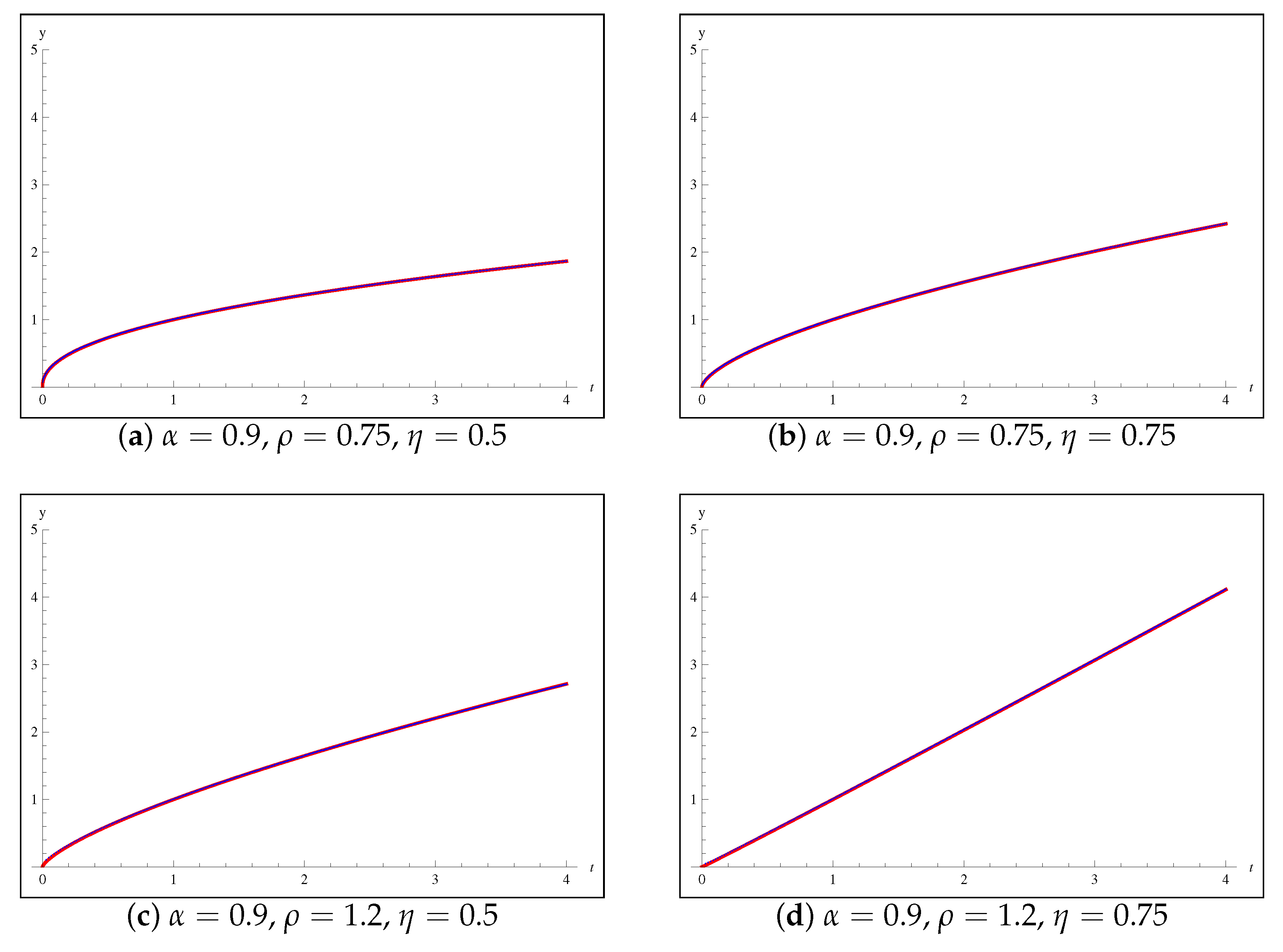
Illustrative Example 2. Our second example covers the Caputo-type E–K initial value problem.

$$\left(D_{0+;\rho ,\eta }^{\alpha }y\right)\left(t\right)=\frac{\mathsf{\Gamma }(2\eta +2)}{\mathsf{\Gamma }(2\eta +2-\alpha )}{t}^{\rho (\eta +1-\alpha )}+y^{3/2}-t^{3\rho (\eta +1-\alpha )/2},y\left(0\right)=0,$$

(55)

where $D_{0+;\rho ,\eta }^{\alpha }$ is the Caputo-type E–K fractional derivative, $\rho >0$, $0<\alpha \le 1$ and $\eta +1>\alpha$. The exact solution of the IVP (55) is $y\left(t\right)=t^{\rho (\eta +1-\alpha )}$. Numerical solutions of the IVP (55) are plotted in Figure 2 when $N=400$ over the interval $[0,4]$ for some certain values of the parameters $\alpha$, $\rho$ and $\eta$. From the numerical data shown in Figure 2, we can notice that the numerical approximate solutions produced using our suggested algorithm exactly match the exact solution.

5. Concluding Remarks

In this paper, we suggested a new modification of the E–K fractional derivative in the sense of the Caputo derivative. From the suggested fractional derivative formulation approach, some important properties and relationships with other E–K fractional derivatives were derived. Then, a predictor corrector algorithm to simulate IVPs with the proposed Caputo-type E–K fractional derivative numerically was introduced.

There are three important points to mention here. First, based on the relations (26) and (36) and Remarks 2, 5 and 6, the proposed adjustment of the E–K fractional derivative appears to be closer to ordinary derivatives than other E–K fractional derivatives. Second, the E–K fractional derivatives are greatly affected by the value of the parameters $\alpha$, $\rho$ and $\eta$, which leads to additional degrees of freedom in the fractional models. Third, our numerical test examples confirmed the validity and performance of the proposed predictor–corrector algorithm, and we also simulated real illustrative examples. Therefore, based on these points, it is hoped that the suggested fractional derivative will find useful implementations in the field of fractional calculus in the future.

References

1. Samko, G.; Kilbas, A.; Marichev, O. Fractional Integrals and Derivatives: Theory and Applications; Gordon and Breach: Amsterdam, The Netherlands, 1993. [Google Scholar]
2. Gorenflo, R.; Mainardi, F. Fractional calculus: Integral and differential equations of fractional order. In Fractals and Fractional Calculus in Continuum Mechanics; Carpinteri, A., Mainardi, F., Eds.; Springer: New York, NY, USA, 1997; pp. 277–290. [Google Scholar]
3. Podlubny, I. Fractional Differential Equations; Academic Press: San Diego, CA, USA, 1999. [Google Scholar]
4. Hilfer, R. Applications of Fractional Calculus in Physics; World Scientific Publishing Company: Singapore, 2000. [Google Scholar]
5. Kilbas, A.A.; Srivastava, H.M.; Trujillo, J.J. Theory and Applications of Fractional Differential Equations; Elsevier: Amsterdam, The Netherlands, 2006. [Google Scholar]
6. Bonilla, B.; Rivero, M.; Rodríguez-Germá, L.; Trujillo, J.J. Fractional differential equations as alternative models to nonlinear differential equations. Appl. Math. Comput. 2007, 10, 79–88. [Google Scholar] [CrossRef]
7. Erdélyi, A.; Kober, H. Some remarks on Hankel transforms. Q. J. Math. 1940, 11, 212–221. [Google Scholar] [CrossRef]
8. Sneddon, I.N. The use in mathematical physics of Erdélyi-Kober operators and of some of their generalizations. In Fractional Calculus and Its Applications; Ross, B., Ed.; Springer: Berlin/Heidelberg, Germany, 1975. [Google Scholar]
9. Kalla, S.; Kiryakova, V. An H-function generalized fractional calculus based upon compositions of Erdélyi-Kober operators in Lp. Math. Jpn. 1990, 35, 1–21. [Google Scholar]
10. Kiryakova, V. Generalized Fractional Calculus and Applications (Pitman Res. Notes Math. Ser. 301); Longman Scientific & Technical: Harlow, UK, 1994. [Google Scholar]
11. Kiryakova, V.; Al-Saqabi, B. Transmutation method for solving Erdélyi-Kober fractional differintegral equations. J. Math. Anal. Appl. 1997, 221, 347–364. [Google Scholar] [CrossRef] [Green Version]
12. Gorenflo, G.; Luchko, Y.; Mainardi, F. Wright functions as scale-invariant solutions of the diffusion-wave equation. J. Comput. Appl. Math. 2000, 118, 175–191. [Google Scholar] [CrossRef] [Green Version]
13. Pagnini, G. Erdélyi-Kober fractional diffusion. Fract. Calc. Appl. Anal. 2012, 15, 117–127. [Google Scholar] [CrossRef] [Green Version]
14. Wang, J.R.; Dong, X.W.; Zhou, Y. Analysis of nonlinear integral equations with Erdélyi-Kober fractional operator. Commun. Nonlin. Sci. Numer. Simulat. 2012, 17, 3129–3139. [Google Scholar] [CrossRef]
15. Kiryakova, V.; Luchko, Y. Riemann-Liouville and Caputo type multiple Erdélyi-Kober operators. Cent. Eur. J. Phys. 2013, 11, 1314–1336. [Google Scholar] [CrossRef]
16. Darwish, M.A. On Erdélyi-Kober fractional Urysohn-Volterra quadratic integral equations. Appl. Math. Comput. 2016, 273, 562–569. [Google Scholar] [CrossRef]
17. Ntouyas, S.; Tariboon, J. Nonlocal boundary value problems for fractional differential inclusions with Erdélyi-Kober fractional integral boundary conditions. ScienceAsia 2017, 43, 47–55. [Google Scholar] [CrossRef] [Green Version]
18. Mathai, A.M.; Haubold, H.J. Erdélyi-Kober Fractional Calculus: From a Statistical Perspective. Inspired by Solar Neutrino Physics; Springer: Singapore, 2018. [Google Scholar]
19. Luchko, Y.; Trujillo, J. Caputo-type modification of the Erdélyi-Kober fractional derivative. Fract. Calc. Appl. Anal. 2007, 10, 249–267. [Google Scholar]
20. Diethelm, K.; Ford, N.; Freed, A. A predictor–corrector approach for the numerical solution of fractional differential equations. Nonlin. Dyn. 2002, 29, 3–22. [Google Scholar] [CrossRef]
21. Odibat, Z.; Shawagfeh, N. An optimized linearization-based predictor–corrector algorithm for the numerical simulation of nonlinear FDEs. Phys. Scr. 2020, 95, 065202. [Google Scholar] [CrossRef]
22. Odibat, Z.; Baleanu, D. Numerical simulation of initial value problems with generalized Caputo-type fractional derivatives. Appl. Numer. Math. 2020, 165, 94–105. [Google Scholar] [CrossRef]
Figure 1. Plots of numerical solutions to the IVP (54), when N = 400 : ( R e d ) Exact solution; ( B l u e ) Predictor-corrector algorithm numerical solutions.
Fractalfract 05 00121 g001aFractalfract 05 00121 g001b
Figure 2. Plots of numerical solutions to the IVP (55), when N = 400 : ( R e d ) Exact solution; ( B l u e ) Predictor-corrector algorithm numerical solutions.
Fractalfract 05 00121 g002aFractalfract 05 00121 g002b