Generalized Cauchy Process: Difference Iterative Forecasting Model

Abstract

The contribution of this article is mainly to develop a new stochastic sequence forecasting model, which is also called the difference iterative forecasting model based on the Generalized Cauchy (GC) process. The GC process is a Long-Range Dependent (LRD) process described by two independent parameters: Hurst parameter H and fractal dimension D. Compared with the fractional Brownian motion (fBm) with a linear relationship between H and D, the GC process can more flexibly describe various LRD processes. Before building the forecasting model, this article demonstrates the GC process using H and D to describe the LRD and fractal properties of stochastic sequences, respectively. The GC process is taken as the diffusion term to establish a differential iterative forecasting model, where the incremental distribution of the GC process is obtained by statistics. The parameters of the forecasting model are estimated by the box dimension, the rescaled range, and the maximum likelihood methods. Finally, a real wind speed data set is used to verify the performance of the GC difference iterative forecasting model.

1. Introduction

The stochastic sequences exhibit Long-Range Dependent (LRD), if $\mathrm{as} t \to \infty ,$ the (auto)correlation function $Cov\left(x_0,x_t\right)$ decreases to zero like a power function, slowly enough so that ${\sum }_{t=0}^{\infty }Cov\left(x_0,x_t\right)=\infty .$ In recent years, the trend forecasting of stochastic sequences with LRD characteristics has become a hot topic that has attracted the interest of many scholars [1,2,3,4]. A large number of experiments prove that the forecasting methods based on regression analysis [5,6], Gray system [7,8,9], Wiener process [10,11], Markov process [12,13,14], support vector machine [15,16], fuzzy analysis [17,18], and neural network [19,20] cannot describe the LRD characteristics in the forecasting process of the actual stochastic sequences, which leads in low accuracy of forecasting results. Therefore, a stochastic model with LRD characteristics is proposed, such as fractional Gaussian processes and fBm, etc. [21,22,23], which can describe the LRD characteristics of stochastic sequences. A stochastic sequence forecasting model is established based on the stochastic model with LRD characteristics, which can better forecast the stochastic sequence by comprehensively considering the impact of the past and current states on the future state [24,25,26]. M. Li et al., propose the forecasting theory of the time series with LRD characteristics [27].W. Song at al. [28] and Wan-Qing et al. [29] established a forecasting model based on fBm and applied it to the time series forecasting of power load and rolling bearing degradation. The fBm is used to derive a degradation model and forecast the remaining useful life of mechanical equipment [30,31]. Liu et al. [26] establish a forecasting model based on the fractional Levy stable motion. S. Duan et al. [32] use the fractional Levy stable motion forecasting model to forecast the trend of wind speed. Furthermore, the neural networks with LRD characteristics are also applied to the prediction of random sequences. Yadav et al. [33] apply the long short-term memory network to financial stochastic sequence forecasting. The long short-term memory network has also been applied to weather forecasting [34,35].

It is worth noting that the existing stochastic models describe LRD characteristics with a single parameter, e.g., the Hurst parameter $H$ in the fBm [36], or the fractal dimension $D$ [23,37]. However, there is a linear relationship $H=2-D$ between the Hurst parameter $H$ and the fractal dimension $D$, and the two parameters can be substituted for each other [38]. This leads to a single-parameter model that cannot describe well some LRD processes with high Hurst parameter $H$ and high fractal dimension $D$. Furthermore, the fractional Levy stable motion mentioned in the [26] has LRD characteristics only when the relationship between the characteristic index $\alpha$ and Hurst parameter $H$ is $\alpha H>1$. Therefore, the fBm and the fractional Levy stable motions are greatly limited in describing the local irregularities and LRD characteristics of stochastic sequences. To separately describe the local irregularities and LRD characteristics, the two parameters of the stochastic model must be independent of each other. This article introduces a stochastic model with a two-parameter independent and LRD characteristics: the GC process [39,40,41]. In the GC process, the Hurst parameter $H$ is used to describe the global properties of stochastic sequences, e.g., LRD characteristics; the fractal dimension $D$ describes local properties, e.g., local irregularities.

The GC process is a generalization of the Cauchy process and can be described by the Auto-Correlation Function (ACF) and probability density function [38,42]. The ACF of the GC process is represented by the Hurst parameter $H$ and the fractal dimension $D$, where the two parameters are limited to $1\le D<2$ and $0<H<1$, respectively. If the ACF is nonintegrable, the GC process will be considered as an LRD process with $1\le D<2$ and $0.5<H<1$. It is worth noting that ACF reduces from the GC process to the ordinary Cauchy process when $D=1$ and $H=0$. The probability density function of the GC process is expressed by the location parameter $\mu \in \mathbb{R}$, scale parameter $\delta >0$, and tail exponent $0<p\le 2$. When $p=2$, the probability density function reduces from the GC process to the ordinary Cauchy process.

In the financial field, a financial stock price prediction model established by fBm as the interference term of the Ito process is proposed, namely the fractional Black-Scholes model [43,44,45], to predict the trend of stock prices, the methods and ideas of the fBm-driven Ito process applied to financial forecasting are combined. The GC process is taken as an interference diffusion term with LRD characteristics, and the Ito process based on the GC process is established. Then, the fractal linear system proposed by Ortigueira is used to generate the numerical sequence of the GC process [46,47], which is generated by the convolution of the impulse function and white noise. Because there is no explicit expression of incremental distribution for the GC process, the incremental distribution of the GC process is obtained by probability and statistics. Finally, the Ito process obtained by the GC process as a diffusion term, incremental distribution and difference equation are used to establish the difference iterative forecasting model based on the GC process.

The remaining structure of this article is organized as follows. The basic nature of the GC process is introduced in Section 2. Section 3 shows the modeling process of the difference iterative forecasting model based on the GC process. The model parameter estimation method is shown in Section 4. Section 5 verifies the validity of the forecasting model through actual data of wind speed. Section 6 gives the conclusion of this article.

2. GC Process: Properties

2.1. Preliminary Knowledge

Definition 1.

Self-similarity property. A self-similar process is a stochastic process$X\left(t\right)$with the same finite-dimensional distribution globally and locally in a statistical sense, and its mathematical definition is [36,37]:

$$X\left(at\right)\equiv a^{H}X\left(t\right),a>0,$$

(1)

where$\equiv$indicates that both sides of the equation have the same probability distribution,$0<H<1$is a self-similar parameter, also known as Hurst parameter. If Definition 1 holds for all$t$, then$X\left(t\right)$is a global self-similar process.

Definition 2.

ACF. In this article, the ACF of$X\left(t\right)$is represented by$R_{XX}\left(\tau \right)$, whose expression is as follows [21,22]:

$$R_{XX}\left(\tau \right)=E\left[X\left(t\right)X\left(t+\tau \right)\right],$$

(2)

where$\tau$is the time lag and$E[·]$is the mean operator.

Definition 3.

LRD characteristic. If the ACF obeys an asymptotic power function, then$X\left(t\right)$has LRD characteristics, namely [27]:

$$R_{XX}\left(\tau \right)\sim c{\tau }^{-\beta } \left(\tau \to \infty \right),$$

(3)

where$c$is a constant and$0<\beta <1$is the LRD index, which is given by the Hurst parameter:

$$\beta \hspace{0.17em}=\hspace{0.17em}2-2H.$$

(4)

At this time, the Hurst parameter$H$is limited to$0.5<H<1$.

Definition 4.

Fractal dimension. The fractal dimension$D$is related to the fractal index$\alpha$, which represents the local irregularity of$X\left(t\right)$and is defined as [23,28]:

$$R_{XX}\left(0\right)-R_{XX}\left(\tau \right)\sim c_1{\left|\tau \right|}^{\alpha }, \left(\tau \to 0\right),$$

(5)

$$D=2-\frac{\alpha }{2},$$

(6)

where$0<\alpha \le 2$,$1\le D<2$, and$c_1$is a constant with a value greater than 0.

It can be seen from Equations (4) and (6) that the Hurst parameter $H$ and the fractal dimension $D$ represent the global and local properties of the stochastic process $X\left(t\right)$, respectively, because the LRD exponent and the fractal exponent are obtained under the conditions of $\tau \to \infty$ and $\tau \to 0$, respectively.

On the other hand, the Hurst parameter $H$ and the fractal dimension $D$ independently describe the LRD characteristics and local irregularities of stochastic sequences. However, there is a linear relationship between the Hurst parameter $H$ and the fractal dimension $D$ in the fBm [36]:

$$H=2-D.$$

(7)

In other words, the fractal dimension $D$ of fBm increases as the Hurst parameter $H$ decreases, and decreases as the Hurst parameter increases. When both the Hurst parameter $H$ and the fractal dimension $D$ are large, e.g., a stochastic sequence, which has both strong LRD and strong local irregularities, cannot be effectively described by the fBm model.

2.2. GC Process

The probability density function of $X\left(t\right)$ has the following form, which is called Cauchy distribution [39,40]:

$$f_{Cauchy}\left(x\right)=\frac{1}{\pi }\left[\frac{\delta }{{\left(x-\mu \right)}^2+{\delta }^2}\right],$$

(8)

where $X\left(t\right)$ is a stochastic process, $\mu$ is the position parameter and $\delta$ is the scale parameter. The Cauchy class model is obtained by generalizing Cauchy distribution in the autocorrelation domain. Its ACF and fractal dimension are as follows [41]:

$$R_C\left(\tau \right)={\left(1+{\left|\tau \right|}^2\right)}^{H-1},$$

(9)

$$R_C\left(0\right)-R_C\left(\tau \right)\sim {\left|\tau \right|}^2, \left(\tau \to 0\right).$$

(10)

where $R_C\left(\tau \right)$ is ACF of Cauchy class model. From Equations (5), (6) and (10), the fractal dimension of the Cauchy class process is always limited to $D=1$. The stochastic process with the fractal dimension in the range of $\left(1,2\right)$ cannot be described. Therefore, the Cauchy class process is generalized to the GC process. In this article, the GC distribution is extended to the correlation domain to obtain the ACF, thereby defining the GC process.

The GC distribution is defined by the following probability density function form [39,41]:

$$f\left(x\right)=\frac{p\mathsf{\Gamma }\left(2/p\right)\delta }{2{\left(\mathsf{\Gamma }\left(1/p\right)\right)}^2}{\left({\delta }_{}^p+{\left|x-\mu \right|}^p\right)}^{-2/p},$$

(11)

where $\mathsf{\Gamma }\left(x\right)$ is the gamma function and $p$ is the tail constant. It should be noted that the GC distribution reduces into Cauchy distribution when $p\hspace{0.17em}=\hspace{0.17em}2$. The GC distribution is introduced into the correlation domain, and the ACF of the Cauchy class model is further extended to obtain the ACF [38,42]:

$$R_{GC}\left(\tau \right)={\left(1+{\left|\tau \right|}^{4-2D}\right)}^{-\frac{1-H}{2-D}}.$$

(12)

That is, the stationary Gaussian process with the ACF of the Equation (12) is called the GC process.

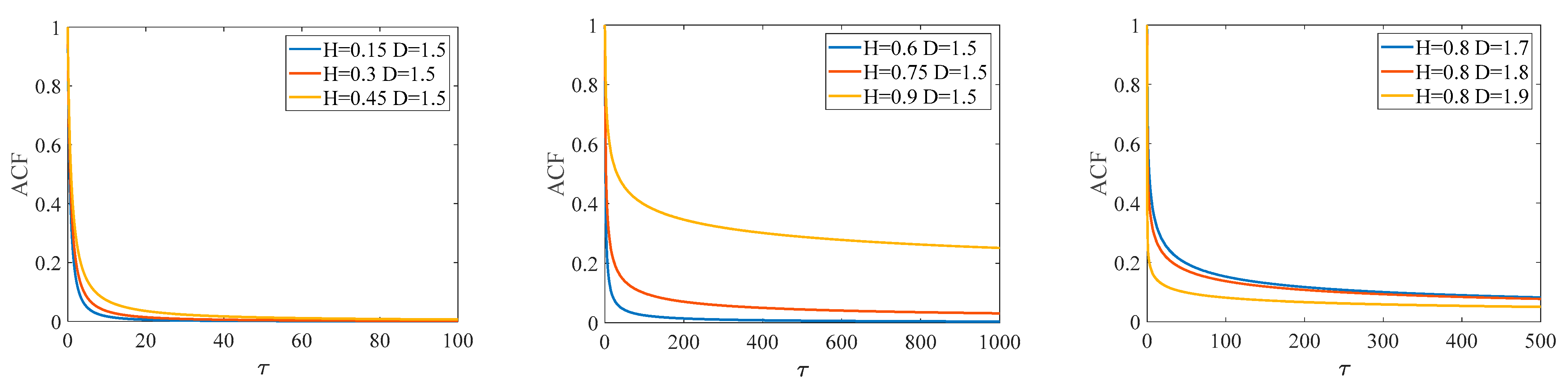
2.2.1. The LRD Characteristics of the GC Process

Compared with single-parameter stochastic models, such as fBm, the GC model can describe the correlation of stochastic sequences by two parameters, e.g., the GC process is an LRD process when $1\le D<2$ and $0.5<H<1$. Figure 1 shows the ACF curves of the GC process under different parameter values, which show the influence of different Hurst parameters and fractal dimensions on the correlation. On the one hand, the effect of the Hurst parameter on the ACF is global and determines the overall trend. On the other hand, the influence of the fractal dimension on the ACF is local, and the influence on the global behaviors is small.

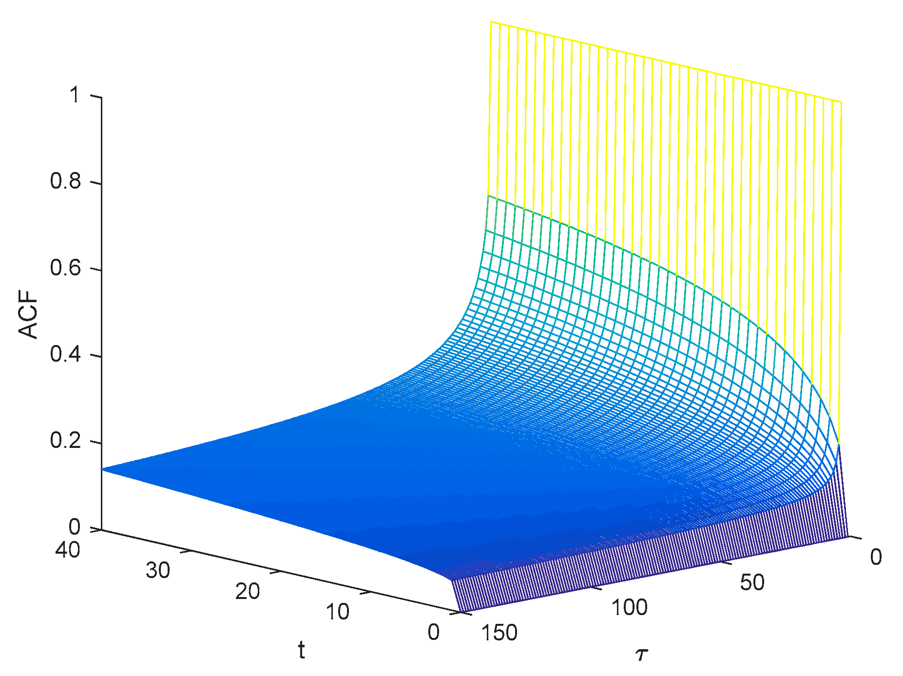
2.2.2. Self-Similarity Properties of the GC Process

Unlike the global self-similarity of fBm, the GC process has only weak self-similarity properties, that is, local self-similarity (relative to the global self-similarity property of Equation (1)), which is defined as [38]:

$$X\left(s\right)-X\left(at\right)\equiv a^H\left[X\left(s\right)-X\left(at\right)\right],\left|t-s\right|\to 0.$$

(13)

where $a$ is a constant.

In [41], it is proposed that the GC process can be transformed into a global self-similar process through Lamperti transformation. Let $Y\left(t\right)$ be the GC process after transformation; then, the transformation form is:

$$Y\left(t\right)=t^{H}X\left(\ln t\right),t>0$$

(14)

The ACF of $Y\left(t\right)$ is shown in Figure 2.

2.3. The Generation of the GC Sequence

Ortigueira fractal linear system theory shows that a steady-state time series can be obtained by white noise and filters, the specific process being [46,47]:

$$x\left(t\right)=w\left(t\right)\times h\left(t\right)={\displaystyle {\int }_0^{t}h\left(t-\tau \right)}w\left(\tau \right)d\tau ,$$

(15)

where $w\left(t\right)$ is the white noise, $h\left(t\right)$ is the impulse function and $x\left(t\right)$ is the generated stationary time series. Similarly, a non-stationary white noise can be passed through a linear filter to obtain a non-stationary time series. This article introduces a method to generate GC sequence by Gaussian white noise and impulse function. The GC sequence is generated as follows:

Step 1: Calculating the Fourier transform of Equation (15).

$$X_{GC}\left(\omega \right)=W\left(\omega \right)H_{GC}\left(\omega \right),$$

(16)

where $X_{GC}\left(\omega \right)$, $W_{GC}\left(\omega \right)$ and $H_{GC}\left(\omega \right)$ are the Fourier transforms of $x_{GC}\left(t\right)$, $w\left(t\right)$ and $h_{GC}\left(t\right)$, respectively.

Step 2: Calculating $H_{GC}\left(\omega \right)$

$$H_{GC}\left(\omega \right)=F{\left({\left(1+{\left|t\right|}^{4-2D}\right)}^{-\frac{1-H}{2-D}}\right)}^{0.5},$$

(17)

where $F\left[x\right]$ is the Fourier transform operator.

Step 3: Calculating the inverse Fourier transform of $H_{GC}\left(\omega \right)$ to find the impulse function:

$$h_{GC}\left(t\right)=F^{-1}\left[F{\left({\left(1+{\left|\tau \right|}^{4-2D}\right)}^{-\frac{1-H}{2-D}}\right)}^{0.5}\right],$$

(18)

where $F^{-1}\left[x\right]$ is the inverse Fourier transform operator. The impulse function at $D=1.5$ and $H=0.6$ is shown in Figure 3.

Figure 4 and Figure 5 show the simulation sequence generated by the GC process. Figure 4 shows that the global trend of the sequence is approximately the same under the same Hurst parameter, but the higher fractal dimension will result in stronger local irregularities (Figure 4b). Figure 5 shows that the local irregularity of the sequence is similar under the same fractal dimension, but the sequence with a higher Hurst parameter has a stronger global trend (Figure 5b).

3. The Difference Iterative Forecasting Model Based on the GC Process

Brownian motion is a stochastic process in the mathematical sense [28], which can be described by the stochastic differential equation, whose expression is as follows:

$$dB\left(t\right)=w\left(t\right)dt,$$

(19)

where $B\left(t\right)$ is Brownian motion. Then, Equation (20) is extended to the Ito process with drift and interference terms [43,48]:

$$dX\left(t\right)=\mu dt+\delta dB\left(t\right),$$

(20)

where $X\left(t\right)$ is the stochastic sequence, $\mu$ and $\delta$ are the drift rate and interference intensity (or volatility).

Scholes and F. Black [44], and Wang at el. [45] gave the fBm $B_H\left(t\right)$ instead of $B\left(t\right)$ as the volatility term of the Ito process and established the Black-Scholes model to describe the trend of the financial option $S_t$:

$$d{S}_t=\mu S_{t}dt+\delta S_{t}d{B}_H\left(t\right)$$

(21)

where $B_H\left(t\right)$ is the fBm. These articles apply the concept of forecasting in the financial field to the stochastic sequences.

The Black-Scholes model assumes that the volatility value is constant, which does not conform to the phenomenon that the non-stationarity of the stochastic sequence causes the trend to change over time, and it cannot explain the influence of local volatility on long-term dependence. In order to solve this problem, the expression of the Ito process is extended. The constants $\mu$ and $\delta$ are extended to time-dependent functions $\mu \left(t\right)$ and $\delta \left(t\right)$, respectively; the interference term $B\left(t\right)$ is represented by $Z\left(t\right)$, which is defined as follows:

$$dX\left(t\right)=\mu \left(t\right)dt+\delta \left(t\right)dZ\left(t\right).$$

(22)

From the perspective of the Ito process driven by the fBm, the GC process can be regarded as a stochastic interference term with LRD properties. Therefore, the generalized expression of the Ito process driven by the fBm is as follows:

$$dX\left(t\right)=\mu \left(t\right)dt+\delta \left(t\right)dGC\left(t\right).$$

(23)

$\mu \left(t\right)$ is the drift coefficient, which represents the global trend of the GC process; $\delta \left(t\right)$ is the diffusion coefficient, which represents the local uncertainty of the GC process.

The stochastic sequence forecasting model based on the GC process is obtained by combining Equations (22) and (24), and the form is as follows

$$dX\left(t\right)=\mu \left(t\right)X\left(t\right)dt+\delta \left(t\right)X\left(t\right)dGC\left(t\right).$$

(24)

Discretizing the Equation (25), we can get:

$$\Delta X\left(t\right)=\mu X\left(t\right)\Delta t+\delta X\left(t\right)\Delta GC\left(t\right),$$

(25)

where $\Delta GC\left(t\right)=GC\left(t+\tau \right)-GC\left(t\right)$. The distribution of the GC process increments $\Delta GC\left(t\right)$ can be obtained through statistical reasoning. The specific process is as follows:

Step 1: The numerical sequence of the GC process is generated by Equation (19).

Step 2: Difference between two states with a time interval $\tau$ is computed, namely,

$$\Delta GC\left(t\right)=GC\left(t+\tau \right)-GC\left(t\right)$$

(26)

Step 3: Step 2 is repeated for the time series generated by Step 1, and multiple differences are made to construct an incremental set.

Step 4: Calculating the variance ${\delta }_{\tau }$ of the incremental distribution. The GC process is a stationary Gaussian process and the increment of interval $\tau$ also follows the Gaussian distribution, i.e., $\Delta GC\left(t\right)\sim N\left(0,{\delta }_{\tau }\right)$, as shown in Figure 6.

Therefore,

$$\Delta GC\left(t\right)=GC\left(t+\tau \right)-GC\left(t\right)\sim N\left(0,{\delta }_{\tau }\right),$$

(27)

Substituting Equation (26) into the difference equation:

$$\Delta X\left(t\right)=X\left(t+1\right)-X\left(t\right).$$

(28)

The difference iterative forecasting model is obtained:

$$X\left(t+1\right)=X\left(t\right)+\mu X\left(t\right)\Delta t+\sigma X\left(t\right)\Delta GC\left(t\right),$$

(29)

where $\Delta GC\left(t\right)\sim N\left(0,{\delta }_{\tau }\right)$. Let $H=0.75$, $D=1.5$, $\mu =0.28$, $\delta =0.35$, ${\delta }_{\tau }=0.32$. Substituting these parameters into Equation (31) and performing 100 Monte Carlo simulations, the generated numerical sequence is similar to the sequence generated by the GC process, as shown in Figure 7.

4. Parameter Estimation of Difference Iterative Forecasting Model

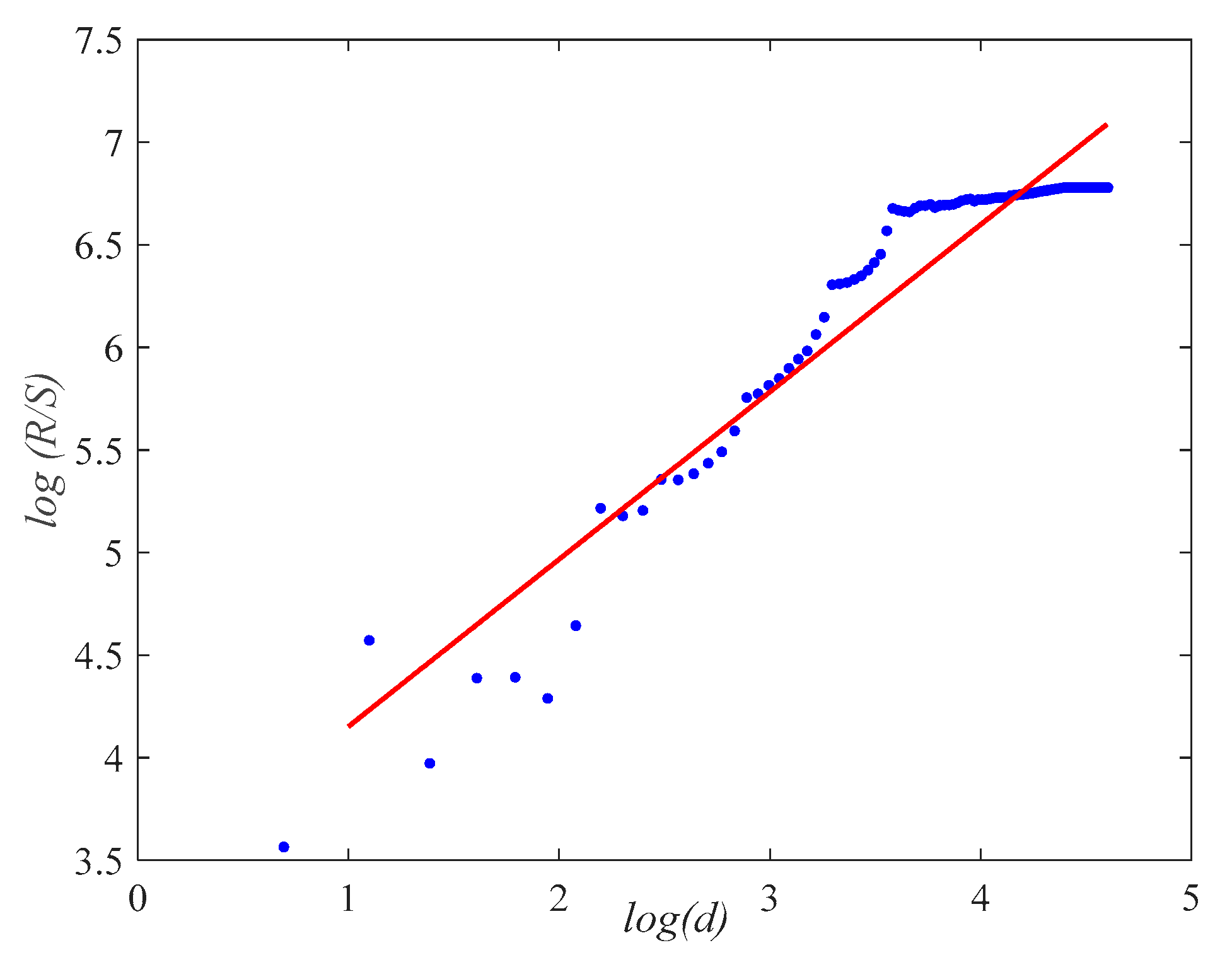
4.1. Estimated Hurst Parameter H

There are many existing methods for estimating the Hurst parameter, such as the periodic graph method, the variance method and the absolute value method [29]. A commonly used method is called the rescaled range method [26]. In the process of estimating the Hurst parameter by the rescaled range method, the input sample sequence is divided into subsequences of the same length, and the average value of the ratio of the standard deviation and the range is calculated for the subsequence, e.g., the rescaled range; the length of the subsequence is re-divided to calculate the rescaled range; all the rescaled ranges and the corresponding subsequence lengths takes the logarithm, and the estimated value of the Hurst parameter is obtained by least-squares fitting (see Figure 8). The mathematical definition is as follows:

$$\log \left[\frac{R}{S}\left(d\right)\right]=H\times \log \left(d\right)+\log \left(c\right)+\varsigma ,$$

(30)

where $d$ is the length of different subsequences, $c$ is a constant, $\varsigma$ is the error, $R$ is the range, $S$ is the standard deviation, $\frac{R}{S}\left(d\right)$ is the rescaled range and $H$ is the Hurst parameter estimate.

4.2. Estimated Fractal Dimension D

There are some techniques commonly used to estimate fractal dimensions, such as box counting and spectroscopy [49]. However, some of these methods, such as spectrometry, have some errors. In this article, we will use the box-dimension method to calculate the fractal dimension [50,51]. The box dimension method divides the plane of the sample sequence into small lattices; then, it takes the logarithm of the total number of lattices covering the sample sequence and the corresponding lengths and obtains the estimated value of the fractal dimension by least-square fitting (as shown in Figure 9). The specific mathematical definition of the box-counting method is as follows:

$$\log \left(N_e\right)=D\times \log \left(1/e\right)+\log \left(c\right)+\varsigma ,$$

(31)

where $N_e$ is the number of grids covering the sample sequence, $e$ is the corresponding side length of the grid, and $D$ is the estimated value of the fractal dimension.

4.3. Estimated Drift and Diffusion Coefficients

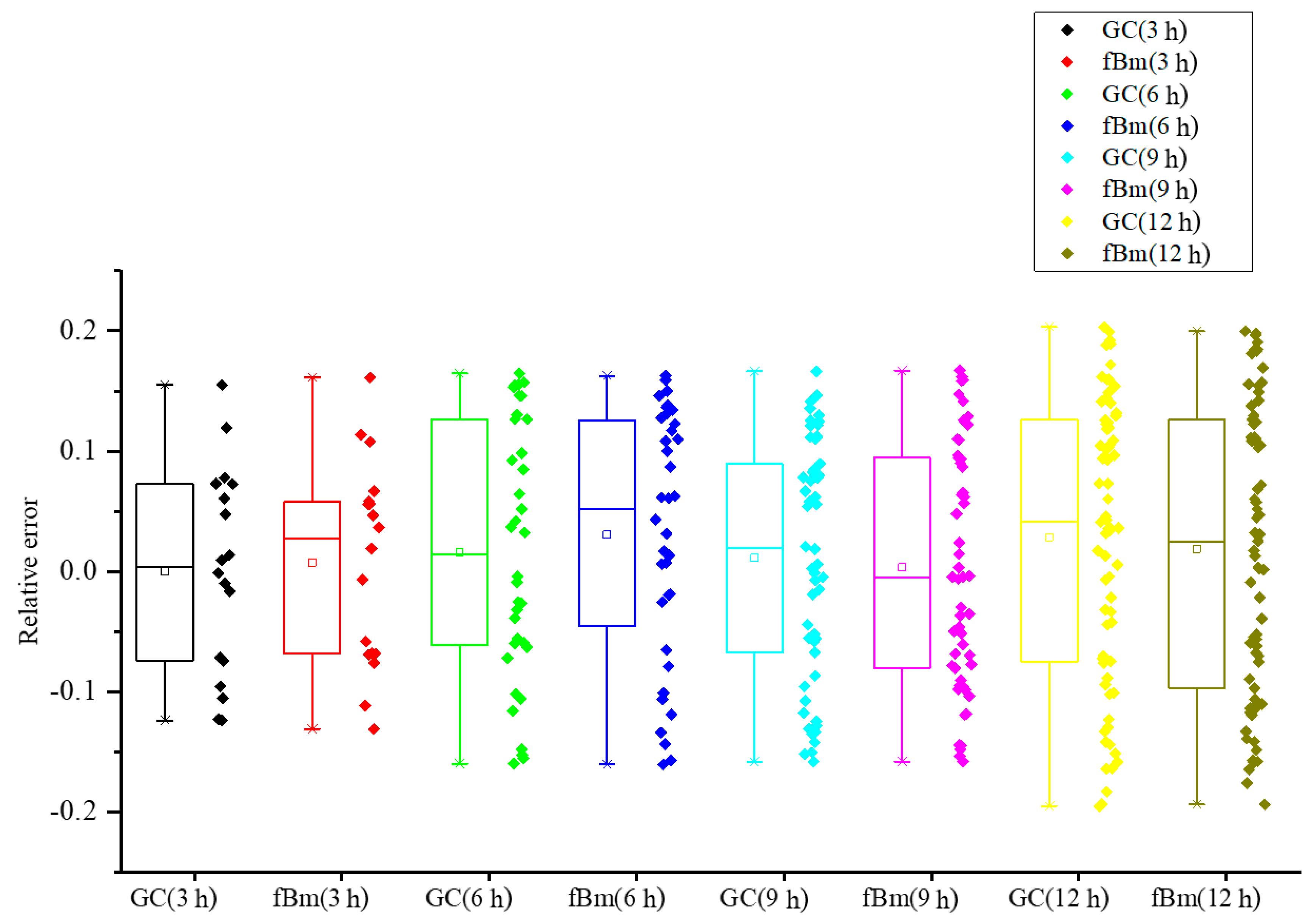
The establishment of the difference iterative prediction model not only relies on Hurst parameter and fractal dimension to generate GC sequence but also requires drift coefficient and diffusion coefficient to establish the stochastic differential equation. Therefore, the probability density function of the GC process is calculated by the maximum likelihood estimation method [42,52] to estimate the values of the drift and diffusion coefficients.

Let $x=\left[x_1,x_2,\cdots ,x_n\right]$ be a set of input sample sequences with unknown parameters $\mu$ and $\delta$; then, the unknown parameters can be obtained by maximum likelihood estimation:

$$\left(\widehat{\mu },\widehat{\delta },p\right)=\arg \underset{\mu ,\delta ,p}{\max }f\left(x;\mu ,\delta ,p\right),$$

(32)

where $f\left(x;\mu ,\delta ,p\right)$ is the joint probability distribution of the GC process, which is defined as:

$$\begin{array}{l}f\left(x;\mu ,\delta ,p\right)=f\left(x_1,x_2,\cdots ,x_i,\cdots ,x_n\right)\\ ={\displaystyle \prod _{i=1}^n}\frac{p\mathsf{\Gamma }\left(2/p\right)\delta }{2{\left(\mathsf{\Gamma }\left(1/p\right)\right)}^2}{\left({\delta }_{}^p+{\left|x_i-\mu \right|}^p\right)}^{-2/p},\end{array}$$

(33)

Taking logarithms on both sides of the equation of Equation (33), then solving the partial derivatives for $\mu ,\delta ,p$ and making the partial derivatives equal to 0:

$$\frac{\partial f}{\partial \mu }={\displaystyle \sum _{i=1}^n\frac{-p{\left|x_i-\mu \right|}^{p-1}\mathrm{sgn}\left(x_i-\mu \right)}{{\delta }_{}^p+{\left|x_i-\mu \right|}^p}}=0,$$

(34)

$$\frac{\partial f}{\partial \delta }={\displaystyle \sum _{i=1}^n\frac{{\delta }_{}^p-{\left|x_i-\mu \right|}^p}{{\delta }_{}^p+{\left|x_i-\mu \right|}^p}}=0,$$

(35)

$$\frac{\partial f}{\partial p}={\displaystyle \sum _{i=1}^n\left[\begin{array}{l}\frac{1}{2p}-\frac{{\delta }_{}^p\log \delta -{\left|x_i-\mu \right|}^p\log \left|x_i-\mu \right|}{p\left({\delta }_{}^p-{\left|x_i-\mu \right|}^p\right)}\\ -\frac{\log \left[{\delta }_{}^p+{\left|x_i-\mu \right|}^p\right]}{p^2}-\frac{1}{p^2}\mathsf{\Psi }\left(\frac{2}{p}\right)+\frac{1}{p^2}\mathsf{\Psi }\left(\frac{1}{p}\right)\end{array}\right]}=0,$$

(36)

where $f=f\left(x;\mu ,\delta ,p\right)$, $\mathsf{\Psi }\left(x\right)$ is the digamma function, defined as $d\ln \mathsf{\Gamma }\left(x\right)/dx$. The estimated values of $\mu ,\delta$ are calculated by using the iterated conditional mode algorithm [42] for Equations (34)–(36).

5. Case Study

To verify the effectiveness of the difference iterative forecasting model based on the GC process, we consider the problem of forecasting the trend of wind speed. In this experiment, the wind speed data set collected by Sotavento Galicia, S.A. company (Galicia, Spain) [53] from 0:00 to 12:00 on 24 February 2020, every ten minutes is used as the sample data for the forecasting model, and forecasts for the next 3 h, 6 h, 9 h and 12 h wind speed trend are given when wind speed data in the previous 12 h are historical data. The parameter estimation method described in Section 4 is used to estimate the model parameters, whose values are given in

Table 1. Parameter estimates of the forecasting model.

	$\mathit{H}$	$\mathit{D}$	$\mathit{\mu }$	$\mathit{\delta }$	${\mathit{\delta }}_{\mathit{\tau }}$
GC	0.8293	1.3650	0.0025	0.0143	0.0103
fBm	0.8293	/	−0.3702	0.5793	/

. The wind speed forecasting is shown in Figure 10. In this experiment, the fBm difference iterative forecasting model is used as a comparative experiment. For the modeling process of fBm, see [28].

Figure 10 shows that the difference iterative forecasting model based on the GC process and the fBm can accurately forecast the wind speed trend.

Table 2. Error analysis of the two forecasting models.

	MAX	MIN	Mean	Median	Mode	SID	MAPE (%)
GC (3h)	0.0169	0.0002	0.0087	0.0005	0.0169	0.0106	0.87
fBm (3h)	0.0196	0.0010	0.0093	0.0034	0.0139	0.106	0.93
GC (6h)	0.0287	0.0006	0.0133	0.0019	0.0239	0.0151	1.33
fBm (6h)	0.0303	0.0011	0.0136	0.0067	0.0264	0.0154	1.36
GC (9h)	0.0350	0.0002	0.0133	0.0030	0.0349	0.0158	1.33
fBm (9h)	0.0366	0.0004	0.0146	0.0060	0.0358	0.0169	1.37
GC (12h)	0.0427	0.0006	0.0146	0.0053	0.0332	0.0169	1.46
fBm(12h)	0.0434	0.0002	0.0153	0.0025	0.0313	0.0184	1.53

: The prediction error results in Table 2 illustrate that the GC difference iterative forecasting model is superior to fBm from three aspects. the local level (maximum, minimum and standard deviation), overall level (mean, median and mode) of the forecasting results, and the fitting effect of the forecasting model (Mean Absolute Percentage Error (MAPE)). Figure 11 shows the boxplot of the relative errors of the two models. No outliers were detected in the figure, thus verifying the effectiveness of GC and FBM iterative prediction models. Further, as shown in Table 1, there are two self-similar parameters $H$ and fractal dimension $D$ in GC model to describe the sequence trend, which respectively predict the global and local trend of the sequence. However, FBM only has self-similar parameter H to predict the global trend of the sequence, so in theory, the prediction accuracy of GC iteration model is higher than that of FBM.

6. Conclusions

In this study, a difference iterative forecasting model is developed from the two-parameter model generalized Cauchy process and it is applied to the changing trend of wind speed. The main contributions are as follows:

• The properties of the Hurst parameter $H$ and fractal dimension $D$ of the generalized Cauchy process are analyzed by the ACF, which describes the global and local properties of stochastic sequences, that is, long-range dependent characteristics and local irregularities, respectively;
• The simulation sequence of the generalized Cauchy process is generated by the white noise through the impulse function, and the incremental distribution of the generalized Cauchy process is obtained by statistical reasoning;
• The Ito process of the generalized Cauchy process is derived through the fractional Black–Schole model; then, the difference iterative forecasting model is established;
• The analysis of the relative error of forecasting results obtained in the wind speed case study considered that the difference iterative forecasting model based on the generalized Cauchy process has good forecasting performance.

References

1. Konar, A.; Bhattacharya, D. Time-Series Prediction and Applications. In Intelligent Systems Reference Library; Springer Nature Switzerland AG: Cham, Switzerland, 2017; Volume 127. [Google Scholar]
2. Fontes, X.; Silva, D. Hybrid Approaches for Time Series Prediction. In Hybrid Intelligent Systems. HIS 2018. Advances in Intelligent Systems and Computing; Springer: Cham, Switzerland, 2018; Volume 923, pp. 146–155. [Google Scholar]
3. Safari, N.; Chung, C.Y.; Price, G.C.D. Novel Multi-Step Short-Term Wind Power Prediction Framework Based on Chaotic Time Series Analysis and Singular Spectrum Analysis. IEEE Trans. Power Syst. 2018, 33, 590–601. [Google Scholar] [CrossRef]
4. Song, W.; Li, M.; Liang, J.-K. Prediction of Bearing Fault Using Fractional Brownian Motion and Minimum Entropy Deconvolution. Entropy 2016, 18, 418. [Google Scholar] [CrossRef] [Green Version]
5. Zhang, Y.; Zhao, Y.; Kong, C.; Chen, B. A new prediction method based on VMD-PRBF-ARMA-E model considering wind speed characteristic. Energy Convers. Manag. 2020, 203, 112254. [Google Scholar] [CrossRef]
6. Xu, W.; Peng, H.; Zeng, X.; Zhou, F.; Tian, X.; Peng, X. Deep belief network-based AR model for nonlinear time series forecasting. Appl. Soft Comput. 2019, 77, 605–621. [Google Scholar] [CrossRef]
7. Yang, X.; Fang, Z.; Yang, Y.; Mba, D.; Li, X. A novel multi-information fusion grey model and its application in wear trend prediction of wind turbines. Appl. Math. Model. 2019, 71, 543–557. [Google Scholar] [CrossRef]
8. Ding, S.; Hipel, K.W.; Dang, Y.-G. Forecasting China’s electricity consumption using a new grey prediction model. Energy 2018, 149, 314–328. [Google Scholar] [CrossRef]
9. Kayacan, E.; Ulutas, B.; Kaynak, O. Grey System Theory-Based Models in Time Series Prediction. Expert Syst. Appl. 2010, 37, 1784–1789. [Google Scholar] [CrossRef]
10. Wang, X.; Balakrishnan, N.; Guo, B. Residual life estimation based on a generalized Wiener degradation process. Reliab. Eng. Syst. Saf. 2014, 124, 13–23. [Google Scholar] [CrossRef]
11. Cheng, Y.; Zhu, H.; Hu, K.; Wu, J.; Shao, X.; Wang, Y. Reliability prediction of machinery with multiple degradation characteristics using double-Wiener process and Monte Carlo algorithm. Mech. Syst. Signal Process. 2019, 134, 106333. [Google Scholar] [CrossRef]
12. Sheng, L.; Cheng, W.; Xia, H.; Wu, X.; Zhang, X. Prediction of annual precipitation based on fuzzy and grey Markov process. In Proceedings of the 2010 International Conference on Machine Learning and Cybernetics, Qingdao, China, 11–14 July 2010; Volume 3, pp. 1136–1140. [Google Scholar]
13. Manoj, J. Application of Markov Process for Prediction of Stock Market Performance. Int. J. Recent Technol. Eng. 2020, 8, 2277–3878. [Google Scholar]
14. Zaki, J.F.; Ali-Eldin, A.; Hussein, S.E.; Saraya, S.F.; Areed, F.F. Traffic congestion prediction based on Hidden Markov Models and contrast measure. Ain Shams Eng. J. 2019, 11, 535–551. [Google Scholar] [CrossRef]
15. Feng, Z.K.; Niu, W.J.; Tang, Z.Y.; Jiang, Z.Q.; Xu, Y.; Liu, Y.; Zhang, H.R. Monthly runoff time series prediction by variational mode decomposition and support vector machine based on quantum-behaved particle swarm optimization. J. Hydrol. 2020, 583, 124627. [Google Scholar] [CrossRef]
16. Li, C.; Lin, S.; Xu, F.; Liu, D.; Liu, J. Short-term wind power prediction based on data mining technology and improved support vector machine method: A case study in Northwest China. J. Clean. Prod. 2018, 205, 909–922. [Google Scholar] [CrossRef]
17. Han, M.; Zhong, K.; Qiu, T.; Han, B. Interval Type-2 Fuzzy Neural Networks for Chaotic Time Series Prediction: A Concise Overview. IEEE Trans. Cybern. 2018, 49, 2720–2731. [Google Scholar] [CrossRef]
18. Ho, D.T.; Garibaldi, J.M. Context-Dependent Fuzzy Systems with Application to Time-Series Prediction. IEEE Trans. Fuzzy Syst. 2014, 22, 778–790. [Google Scholar] [CrossRef]
19. Quan, H.; Srinivasan, D.; Khosravi, A. Short-Term Load and Wind Power Forecasting Using Neural Network-Based Prediction Intervals. IEEE Trans. Neural Netw. Learn. Syst. 2014, 25, 303–315. [Google Scholar] [CrossRef]
20. Zhang, Y.; Chen, B.; Zhao, Y.; Pan, G. Wind Speed Prediction of IPSO-BP Neural Network Based on Lorenz Disturbance. IEEE Access 2018, 6, 53168–53179. [Google Scholar] [CrossRef]
21. Mandelbrot, B.B.; van Ness, J.W. Fractional Brownian Motions, Fractional Noises and Applications. SIAM Rev. 1968, 10, 422–437. [Google Scholar] [CrossRef]
22. Samorodnitsky, G.; Taqqu, M. Stable Non-Gaussian Random Processes: Stochastic Models with Infinite Variance. J. Am. Stat. Assoc. 1996, 90, 123–138. [Google Scholar]
23. Li, M. Fractal Time Series—A Tutorial Review. Math. Probl. Eng. 2010, 2010, 1–26. [Google Scholar] [CrossRef]
24. Sottinen, T.; Viitasaari, L. Prediction Law of fractional Brownian Motion. Stat. Probab. Lett. 2017, 129, 155–166. [Google Scholar] [CrossRef] [Green Version]
25. Li, Q.; Liang, S.; Yang, J.; Li, B. Long Range Dependence Prognostics for Bearing Vibration Intensity Chaotic Time Series. Entropy 2016, 18, 23. [Google Scholar] [CrossRef] [Green Version]
26. Liu, H.; Song, W.; Li, M.; Kudreyko, A.; Zio, E. Fractional Levy stable motion: Finite difference iterative forecasting model. Chaos Solitons Fract. 2020, 133, 109632. [Google Scholar] [CrossRef]
27. Li, M.; Jia-Yue, L. On the Predictability of Long-Range Dependent Series. Math. Probl. Eng. 2010, 2010, 1–9. [Google Scholar] [CrossRef]
28. Song, W.; Li, M.; Li, Y.; Cattani, C.; Chi, C.-H. Fractional Brownian motion: Difference iterative forecasting models. Chaos Solitons Fract. 2019, 123, 347–355. [Google Scholar] [CrossRef]
29. Wan-Qing, S.; Cheng, X.; Cattani, C.; Zio, E. Multi-Fractional Brownian Motion and Quantum-Behaved Partial Swarm Optimization for Bearing Degradation Forecasting. Complexity 2019, 2020, 1–9. [Google Scholar]
30. Zhang, H.; Chen, M.; Xi, X.; Zhou, D. Remaining Useful Life Prediction for Degradation Processes with Long-Range Dependence. IEEE Trans. Reliab. 2017, 66, 1–12. [Google Scholar] [CrossRef]
31. Wang, H.; Song, W.; Zio, E.; Kudreyko, A.; Zhang, Y. Remaining useful life prediction for Lithium-ion batteries using fractional Brownian motion and Fruit-fly Optimization Algorithm. Measurement 2020, 161, 107904. [Google Scholar] [CrossRef]
32. Duan, S.; Wanqing, S.; Cattani, C.; Yasen, Y.; Liu, H. Fractional Levy Stable and Maximum Lyapunov Exponent for Wind Speed Prediction. Symmetry 2020, 2020, 605. [Google Scholar] [CrossRef]
33. Yadav, A.; Jha, C.K.; Sharan, A. Optimizing LSTM for time series prediction in Indian stock market. Proc. Comput. Sci. 2020, 167, 2091–2100. [Google Scholar] [CrossRef]
34. Li, Y.; Zhu, Z.; Kong, D.; Han, H.; Zhao, Y. EA-LSTM: Evolutionary attention-based LSTM for time series prediction. Knowl. Based Syst. 2019, 181, 104785. [Google Scholar] [CrossRef] [Green Version]
35. Karevan, Z.; Suykens, J.A.K. Transductive LSTM for time-series prediction: An application to weather forecasting. Neural Netw. 2020, 125, 1–9. [Google Scholar] [CrossRef]
36. Song, W.; Cattani, C.; Chi, C.-H. Multifractional Brownian motion and quantum-behaved particle swarm optimization for short term power load forecasting: An integrated approach. Energy 2020, 194, 116847. [Google Scholar] [CrossRef]
37. Schlager, W. Fractal nature of stratigraphic sequences. Geology 2004, 32, 185–188. [Google Scholar] [CrossRef]
38. Li, M.; Li, J.-Y. Generalized Cauchy model of sea level fluctuations with long-range dependence. Phys. A Stat. Mech. Appl. 2017, 484, 309–335. [Google Scholar] [CrossRef]
39. Liu, H.; Song, W.-Q.; Zio, E. Generalized Cauchy difference iterative forecasting model for wind speed based on fractal time series. Nonlinear Dyn. 2021, 103, 759–773. [Google Scholar] [CrossRef]
40. Li, M. Multi-fractional generalized Cauchy process and its application to teletraffic. Phys. A Stat. Mech. Appl. 2020, 550, 123982. [Google Scholar] [CrossRef]
41. Lim, S.; Li, M. A generalized Cauchy process and its application to relaxation phenomena. J. Phys. A Math. Gen. 2006, 39, 2935. [Google Scholar] [CrossRef]
42. Carrillo, R.; Aysal, T.; Barner, K. A Generalized Cauchy Distribution Framework for Problems Requiring Robust Behavior. EURASIP J. Adv. Signal Process. 2010, 2010, 312989. [Google Scholar] [CrossRef] [Green Version]
43. Dai, W.; Heyde, C.C. Itô’s formula with respect to fractional Brownian motion and its application. J. Appl. Math. Stoch. Anal. 1996, 9, 439–448. [Google Scholar] [CrossRef] [Green Version]
44. Scholes, M.; Black, F. The Pricing of Options and Corporate Liabilities. J. Polit. Econ. 1973, 81, 637–654. [Google Scholar]
45. Wang, X.-T.; Qiu, W.-Y.; Ren, F.-Y. Option pricing of fractional version of the Black–Scholes model with Hurst exponent H being in (1/3,1/2). Chaos Solitons Fract. 2001, 12, 599–608. [Google Scholar] [CrossRef]
46. Ortigueira, M.D. Introduction to fractional linear systems. Part 2. Discrete-time case. In IEE Proceedings—Vision, Image and Signal Processing; IET—Institution of Engineering and Technology: Karnataka, India, 2000; Volume 147, pp. 71–78. [Google Scholar]
47. Ortigueira, M.C. Introduction to fractional linear systems. Part 1. Continuous-time case. In IEE Proceedings—Vision, Image and Signal Processing; IET—Institution of Engineering and Technology: Karnataka, India, 2000; Volume 147, pp. 62–70. [Google Scholar]
48. Yan, L.; Shen, G.; He, K. Itô’s formula for a sub-fractional Brownian motion. Commun. Stoch. Anal. 2011, 5, 135–159. [Google Scholar] [CrossRef] [Green Version]
49. Li, M.; Lim, S.; Feng, H. Generating Traffic Time Series Based on Generalized Cauchy Process. In Proceedings of the International Conference on Computational Science, Beijing, China, 27–30 May 2007; Springer: Berlin/Heidelberg, Germany, 2007; pp. 374–381. [Google Scholar]
50. Panigrahy, C.; Seal, A.; Mahato, N.K.; Bhattacharjee, D. Differential box counting methods for estimating fractal dimension of gray-scale images: A survey. Chaos Solitons Fract. 2019, 126, 178–202. [Google Scholar] [CrossRef]
51. Silva, P.M.; Florindo, J.B. A statistical descriptor for texture images based on the box counting fractal dimension. Phys. A Stat. Mech. Appl. 2019, 528, 121469. [Google Scholar] [CrossRef]
52. Konno, H.; Watanabe, F. Maximum likelihood estimators for generalized Cauchy processes. J. Math. Phys. 2007, 48, 1–19. [Google Scholar] [CrossRef] [Green Version]
53. Sotavento. Sotavento Technical Area Real Time Data Historical. Available online: http://www.sotaventogalicia.com/en/technical-area/real-time-data/historical/ (accessed on 25 March 2021).
Figure 1. ACF curve of GC process under different parameters.
Fractalfract 05 00038 g001
Figure 2. ACF of GC process after Lamperti transformation.
Fractalfract 05 00038 g002
Figure 3. Impulse function of the generalized Cauchy sequence.
Fractalfract 05 00038 g003
Figure 4. GC sequence generated by the same Hurst parameter. (a) H = 0.55 ,   D = 1.2 ; (b) H = 0.55 ,   D = 1.8 .
Fractalfract 05 00038 g004
Figure 5. GC sequence generated by the same fractal dimension. (a) H = 0.6 ,   D = 1.5 ; (b) H = 0.9 , D = 1.5 .
Fractalfract 05 00038 g005aFractalfract 05 00038 g005b
Figure 6. Numerical simulation of the incremental distribution of the GC process.
Fractalfract 05 00038 g006
Figure 7. Numerical sequence generated by the Monte Carlo method.
Fractalfract 05 00038 g007
Figure 8. Least-squares fitting of Hurst parameter.
Fractalfract 05 00038 g008
Figure 9. Least-squares fitting of fractal dimension.
Fractalfract 05 00038 g009
Figure 10. Comparison of the forecasting trends of the two models. (a) Forecasting the next 3 h; (b) Forecasting the next 6 h; (c) Forecasting the next 9 h; (d) Forecasting the next 12 h.
Fractalfract 05 00038 g010
Figure 11. Boxplot of the relative error of the forecasting models.
Fractalfract 05 00038 g011