Article

Simultaneous Characterization of Relaxation, Creep, Dissipation, and Hysteresis by Fractional-Order Constitutive Models

1
School of Sciences, Shanghai Institute of Technology, Shanghai 201418, China
2
MESA Lab, University of California, Merced, 5200 North Lake Road, Merced, CA 95343, USA
*
Author to whom correspondence should be addressed.
These authors contributed equally to this work.
Fractal Fract. 2021, 5(2), 36; https://doi.org/10.3390/fractalfract5020036
Submission received: 26 March 2021 / Revised: 10 April 2021 / Accepted: 16 April 2021 / Published: 20 April 2021
(This article belongs to the Special Issue Fractal Media and Fractional Viscoelasticity)

Abstract

:
We considered relaxation, creep, dissipation, and hysteresis resulting from a six-parameter fractional constitutive model and its particular cases. The storage modulus, loss modulus, and loss factor, as well as their characteristics based on the thermodynamic requirements, were investigated. It was proved that for the fractional Maxwell model, the storage modulus increases monotonically, while the loss modulus has symmetrical peaks for its curve against the logarithmic scale log ( ω ) , and for the fractional Zener model, the storage modulus monotonically increases while the loss modulus and the loss factor have symmetrical peaks for their curves against the logarithmic scale log ( ω ) . The peak values and corresponding stationary points were analytically given. The relaxation modulus and the creep compliance for the six-parameter fractional constitutive model were given in terms of the Mittag–Leffler functions. Finally, the stress–strain hysteresis loops were simulated by making use of the derived creep compliance for the fractional Zener model. These results show that the fractional constitutive models could characterize the relaxation, creep, dissipation, and hysteresis phenomena of viscoelastic bodies, and fractional orders α and β could be used to model real-world physical properties well.

1. Introduction

Theories and applications of fractional calculus have attracted much attention and acquired rapid developments during the last several decades because fractional calculus is appropriate for representing the memory and hereditary properties of materials and processes. Oldham and Spanier [1] completed the first monograph in 1974, and Ross [2] contributed the first proceedings in 1975. To date, the number of monographs and proceedings specializing in fractional calculus and its applications has gone up to several dozens; e.g., [3,4,5,6,7,8,9,10,11,12,13,14,15]. The application areas of fractional calculus include rheology [16], non-Newtonian fluid dynamics [17,18,19], viscoelastic theory [9,20,21,22,23], anomalous diffusion [1,24,25,26,27,28,29,30], control theory [7,31,32,33,34,35], hysteresis phenomena [36], dynamical systems [12,37,38,39,40,41], and so on.
The applications of fractional calculus to viscoelasticity were promoted by the wide use of viscoelastic materials in damping design and shock absorption. Scott-Blair [42,43] presented a fractional constitutive relation σ ( t ) = E ϵ ( α ) ( t ) , where 0 < α < 1 and E and α are material constants for a viscoelastic material that is an intermediate between a pure elastic solid (Hooke model) and a pure viscous fluid (Newton model). In [9,44], this relation was called the Scott-Blair model. Macromolecule materials, such as butyl and polybutadiene, are typical viscoelastic bodies whose constitutive relations can be modeled by using fractional derivatives [45]. Fractional constitutive models, such as the fractional Maxwell, Kelvin–Voigt, and Zener models, were suggested by replacing the classical Newton element with the Scott-Blair element [9,23,45,46,47,48,49,50], i.e., substituting the integer-order derivatives into the fractional-order derivatives. In [51], viscoelastic dampers were simulated by using the Maxwell and Kelvin–Voigt fractional models. In [52], a fractional integral form and differential form were compared for the the standard solid model.
In [53], a fractional five-parameter model was proposed, and it was compatible with the high-frequency metadata. In [54], a fractional six-parameter model was proposed to include all of the four types of viscoelasticity. In [55], energy storage and energy dissipation for the fractional equations were discussed. In [49,56,57,58,59], distributed-order derivatives were introduced to model viscoelastic constitutive equations.
Suppose that f ( t ) is a piecewise continuous function defined on ( 0 , + ) and is integrable on each finite subinterval. Then, the Riemann–Liouville fractional integral of order λ is defined as
I t λ f ( t ) = 0 t ( t τ ) λ 1 Γ ( λ ) f ( τ ) d τ , t > 0 ,
for λ > 0 , and I t λ f ( t ) = f ( t ) for λ = 0 , where Γ ( · ) is the Gamma function. The Riemann–Liouville fractional derivative of order α is defined, when it exists, as
D t α f ( t ) = d m d t m I t m α f ( t ) , t > 0 , m 1 < α m , m N + .
The functions that we considered are causal, viz., identically equal to zero when t < 0 .
We use the Laplace transform with a lower limit of integral 0 ,
f ¯ ( s ) = L [ f ( t ) ] = 0 e s t f ( t ) d t , Re ( s ) > c .
So, the Laplace transform of the Riemann–Liouville fractional derivative satisfies
L [ D t α f ( t ) ] = s α f ¯ ( s ) .
We note that the initial conditions at t = 0 + will not appear in the Laplace transform of the constitutive relation of the stress and strain on the assumption that the contributions from the initial conditions are canceled if the Laplace transform with the starting point t = 0 + is used [9].
The Mittag–Leffler functions are significant in fractional models. These types of functions have the definition [7,60,61]
E λ , μ ( z ) = k = 0 z k Γ ( λ k + μ ) , λ > 0 , μ > 0 .
The following Laplace transform formula holds:
L t λ k + μ 1 E λ , μ ( k ) ( c t λ ) = k ! s λ μ ( s λ + c ) k + 1 , λ > 0 , μ > 0 .
Dissipation and hysteresis phenomena exist broadly in mechanical systems [9,49,62,63,64]. Energy dissipation was considered in some fractional constitutive equations in [9,49,53,55,65]. In [36], fractional-order models were proposed to describe the broadband hysteresis of a piezoelectric actuator by looking into the relationship between the input voltage and the output displacement. Simulations and experiments were performed to validate the effectiveness of the fractional-order model.
The purpose of this work is to consider dissipation, creep, relaxation, and hysteresis for a six-parameter fractional constitutive model and its particular cases. In the next section, we consider the storage modulus, loss modulus, and loss factor, as well as their characteristics for different fractional constitutive models based on the thermodynamic requirements. For the fractional Maxwell model, we prove that the storage modulus increases monotonically, while the loss modulus has symmetrical peaks for its curve against the logarithmic scale log ( ω ) . For the fractional Zener model, we demonstrate that the storage modulus monotonically increases, while the loss modulus and the loss factor have symmetrical peaks for their curves against the logarithmic scale log ( ω ) . In Section 3, the relaxation, creep, and hysteresis for the six-parameter fractional constitutive model are considered by making use of the Mittag–Leffler functions.

2. Fractional Models and Thermodynamic Requirements

We consider the six-parameter fractional constitutive equation
σ ( t ) + a D t α σ ( t ) = b 0 ϵ ( t ) + b 1 D t α ϵ ( t ) + b 2 D t β ϵ ( t ) ,
where the coefficients and the orders are subject to the constraints
a 0 , b k 0 ( k = 0 , 1 , 2 ) , a b 0 b 1 , b 0 , b 1 and b 2 are not all zeros ,
0 < α β 1 .
The creep compliance and relaxation modulus of a six-parameter model similar to that in Equation (7) were considered by using the complex inversion formula of the Laplace transform, and the results were expressed by infinite integrals. In this article, we focus on the thermodynamic requirements in this section and the Mittag–Leffler function expressions of the creep compliance and relaxation modulus in the next section for the six-parameter model (7). Based on these results, the storage modulus, loss modulus, and loss factor are investigated and hysteresis loops are simulated. Operating the Laplace transform for Equation (7) leads to
( 1 + a s α ) σ ¯ ( s ) = ( b 0 + b 1 s α + b 2 s β ) ϵ ¯ ( s ) .
The complex modulus is defined as
G ( ω ) = σ ¯ ( i ω ) ϵ ¯ ( i ω ) = b 0 + b 1 ( i ω ) α + b 2 ( i ω ) β 1 + a ( i ω ) α .
The storage modulus G s and loss modulus G l are defined as the the real part and the imaginary part of the complex modulus
G ( ω ) = G s ( ω ) + i G l ( ω ) .
The loss factor is defined as
ζ ( ω ) = G l ( ω ) G s ( ω ) .
The loss factor is a measure of the damping ability of a linear viscoelastic material. We note that the loss factor is also called loss tangent [9]. The storage modulus G s and loss modulus G l are also denoted as G and G in [9,52,66].
For a constitutive equation of real viscoelastic materials, thermodynamic requirements must be satisfied. It is known from thermodynamics that the internal work and the dissipated energy must be positive. We can satisfy the thermodynamic restrictions by ensuring that both the storage modulus and the loss modulus are positive for all frequencies [65], i.e.,
G s ( ω ) 0 and G l ( ω ) 0 for all ω > 0 .
Inserting the formula i λ = cos ( π λ 2 ) + i sin ( π λ 2 ) into Equation (11) and separating the real part from the imaginary part, we obtain the loss modulus and the storage modulus:
G l ( ω ) = 1 Δ ( b 1 a b 0 ) sin ( π α 2 ) ω α + b 2 sin ( π β 2 ) ω β + a b 2 sin ( π ( β α ) 2 ) ω α + β ,
G s ( ω ) = 1 Δ b 0 + ( b 1 + a b 0 ) cos ( π α 2 ) ω α + b 2 cos ( π β 2 ) ω β + a b 1 ω 2 α + a b 2 cos ( π ( β α ) 2 ) ω α + β ,
where
Δ = 1 + 2 a cos ( π α 2 ) ω α + a 2 ω 2 α .
By using Equations (15) and (16), the following proposition can be directly checked.
Proposition 1.
Under the assumptions in (8) and (9), Equation (7) satisfies the thermodynamic requirements.
The model (7) covers common special cases, including the classical integer-order equations. We firstly list five integer-order equations, as well as their loss and storage moduli and loss factors.
Hook model ( a = b 1 = b 2 = 0 ):
σ ( t ) = b 0 ϵ ( t ) ,
G l = 0 , G s = b 0 , ζ = 0 .
Newton model ( a = b 0 = b 2 = 0 , α = 1 ):
σ ( t ) = b 1 ϵ ˙ ( t ) ,
G l = b 1 ω , G s = 0 , ζ = .
Kelvin–Voigt model ( a = b 2 = 0 , α = 1 ):
σ ( t ) = b 0 ϵ ( t ) + b 1 ϵ ˙ ( t ) ,
G l = b 1 ω , G s = b 0 , ζ = ( b 1 / b 0 ) ω .
Maxwell model ( b 0 = b 2 = 0 , α = 1 ):
σ ( t ) + a σ ˙ ( t ) = b 1 ϵ ˙ ( t ) ,
G l = b 1 ω 1 + a 2 ω 2 , G s = a b 1 ω 2 1 + a 2 ω 2 , ζ = 1 a ω .
Here G s increases monotonically from 0 to b 1 / a , G l has a symmetrical peak for plot with respect to the logarithmic scale log ( ω ) .
Zener model ( b 2 = 0 , α = 1 ):
σ ( t ) + a σ ˙ ( t ) = b 0 ϵ ( t ) + b 1 ϵ ˙ ( t ) ,
G l = ( b 1 a b 0 ) ω 1 + a 2 ω 2 , G s = b 0 + a b 1 ω 2 1 + a 2 ω 2 , ζ = ( b 1 a b 0 ) ω b 0 + a b 1 ω 2 .
Here, G s increases monotonically from b 0 to b 1 / a , and G l and ζ have symmetrical peaks for their plots with respect to the logarithmic scale log ( ω ) .
Next, we consider the fractional cases.
Fractional Scott-Blair model ( a = b 0 = b 2 = 0 ):
σ ( t ) = b 1 D t α ϵ ( t ) ,
G l ( ω ) = b 1 sin ( π α 2 ) ω α , G s ( ω ) = b 1 cos ( π α 2 ) ω α , ζ = tan π α 2 .
The loss modulus and the storage modulus have the same power law with respect to the frequency ω , and the loss factor is independent of ω .
Fractional Kelvin–Voigt model ( a = b 2 = 0 ):
σ ( t ) = b 0 ϵ ( t ) + b 1 D t α ϵ ( t ) ,
G l ( ω ) = b 1 sin ( π α 2 ) ω α ,
G s ( ω ) = b 0 + b 1 cos ( π α 2 ) ω α ,
ζ ( ω ) = b 1 sin ( π α 2 ) ω α b 0 + b 1 cos ( π α 2 ) ω α .
The two moduli G l and G s increase in their power law with respect to ω ; ζ ( ω ) monotonically increases on [ 0 , + ) and satisfies
ζ ( 0 ) = 0 , ζ ( + ) = tan π α 2 .
Before considering new models, we give the following lemma.
Lemma 1.
The function
f ( ω ) = ω α c 0 + c 1 ω α + c 2 ω 2 α , c 0 , c 2 > 0 , c 1 0 , 0 < α 1 , ω 0 ,
has the unique stationary point
ω = c 0 / c 2 1 / ( 2 α ) ,
and the peak value
f ( ω ) = 1 c 1 + 2 c 0 c 2 ,
and f ( ω ) increases monotonically on [ 0 , ω ] and decreases monotonically on [ ω , + ) . For any positive real number p, the following equation holds:
f ( ω p 1 ) = f ( ω p ) .
Proof. 
From the derivative
f ( ω ) = α ω α 1 c 0 c 2 ω 2 α c 0 + c 1 ω α + c 2 ω 2 α 2 ,
we have the stationary point ω , the peak value f ( ω ) in Equation (37), and the monotonicity on the intervals [ 0 , ω ] and [ ω , + ) .
For Equation (38), first, by direct substitution, it is easy to verify that
c 0 p 2 α + c 2 ω 2 α = c 0 + c 2 ( ω p ) 2 α .
Next, we have
f ( ω p 1 ) = ω α p α c 0 + c 1 ω α p α + c 2 ω 2 α p 2 α = ( ω p ) α c 0 p 2 α + c 1 ( ω p ) α + c 2 ω 2 α .
By the relation (39), the Equation (38) is obtained. □
Fractional Maxwell model ( b 0 = b 2 = 0 ):
σ ( t ) + a D t α σ ( t ) = b 1 D t α ϵ ( t ) ,
G l ( ω ) = b 1 sin ( π α 2 ) ω α 1 + 2 a cos ( π α 2 ) ω α + a 2 ω 2 α ,
G s ( ω ) = b 1 cos ( π α 2 ) ω α + a b 1 ω 2 α 1 + 2 a cos ( π α 2 ) ω α + a 2 ω 2 α ,
ζ ( ω ) = b 1 sin ( π α 2 ) b 1 cos ( π α 2 ) + a b 1 ω α .
The loss factor ζ ( ω ) monotonically decreases on [ 0 , + ) and satisfies
ζ ( 0 ) = tan π α 2 , ζ ( + ) = 0 .
For the storage and loss moduli, we give the following proposition.
Proposition 2.
For the fractional Maxwell model (40), the storage modulus G s ( ω ) increases monotonically on the interval [ 0 , + ) and satisfies
G s ( 0 ) = 0 , G s ( + ) = b 1 / a ,
the loss modulus G l ( ω ) has the unique stationary point
ω l = 1 / a 1 / α ,
and the peak value
G l m a x = G l ( ω l ) = b 1 2 a tan ( π α 4 ) ,
has symmetrical peaks for its curve against the logarithmic scale log ( ω ) .
Proof. 
From the derivative
G s ( ω ) = α b 1 ω α 1 cos π α 2 + 2 a ω α + a 2 cos π α 2 ω 2 α 1 + 2 a cos π α 2 ω α + a 2 ω 2 α 2 ,
we know that the storage modulus G s ( ω ) increases monotonically on the interval [ 0 , + ) . Equation (45) is direct from (42). The results for the loss modulus come from Lemma 1. □
Fractional Zener model ( b 2 = 0 ):
σ ( t ) + a D α σ ( t ) = b 0 ϵ ( t ) + b 1 D α ϵ ( t ) ,
G l ( ω ) = ( b 1 a b 0 ) sin ( π α 2 ) ω α 1 + 2 a cos ( π α 2 ) ω α + a 2 ω 2 α ,
G s ( ω ) = b 0 + ( b 1 + a b 0 ) cos ( π α 2 ) ω α + a b 1 ω 2 α 1 + 2 a cos ( π α 2 ) ω α + a 2 ω 2 α ,
ζ ( ω ) = ( b 1 a b 0 ) sin ( π α 2 ) ω α b 0 + ( b 1 + a b 0 ) cos ( π α 2 ) ω α + a b 1 ω 2 α .
First, we notice that when α = 0 , the model becomes the Hook model, and there is no energy dissipation. For the special case a b 0 = b 1 , i.e., the coefficients satisfy the proportional relation 1 / b 0 = a / b 1 , the model stores an invariant energy and has no energy dissipation like a Hook model,
G l ( ω ) = 0 , G s ( ω ) = b 0 .
In the following, we always assume that 0 < α 1 and b 1 > a b 0 .
Proposition 3.
For the fractional Zener model (48), (i) the storage modulus G s ( ω ) monotonically increases on the interval [ 0 , + ) with the limits
G s ( 0 ) = b 0 , G s ( + ) = b 1 / a ;
(ii) the loss modulus G l ( ω ) has the unique stationary point
ω l = 1 / a 1 / α ,
and the peak value
G l m a x = G l ( ω l ) = b 1 a b 0 2 a tan ( π α 4 ) ;
(iii) the loss factor ζ has the unique stationary point
ω f = b 0 a b 1 1 / ( 2 α ) ,
and the peak value
ζ m a x = ζ ( ω f ) = ( b 1 a b 0 ) sin ( π α 2 ) ( b 1 + a b 0 ) cos ( π α 2 ) + 2 a b 0 b 1 ;
(iv) the graphs of the loss modulus and the loss factor against the logarithmic scale log ( ω ) have symmetrical peaks, the stationary points of the loss modulus and the loss factor satisfy the inequality
ω f < ω l ,
the peak values of the loss modulus and loss factor increase monotonically with increasing α and satisfy the inequalities
G l m a x b 1 a b 0 2 a , ζ m a x b 1 a b 0 2 a b 0 b 1 ,
where either of the equal signs holds only if α = 1 , and the two peak values satisfy the relation
a b 1 G l m a x < ζ m a x < 1 b 0 G l m a x .
Proof. 
(i) It is easy to check that the derivative G s ( ω ) 0 . This means that G s ( ω ) is monotonically increasing on the interval [ 0 , + ) . The limits in Equation (53) are directly from (50). (ii) and (iii) result from Lemma 1. (iv) From Equation (38) in Lemma 1, we know that the graphs of the loss modulus and the loss factor against the logarithmic scale log ( ω ) have symmetrical peaks. By the hypothesis b 1 > a b 0 , we have b 0 / ( a b 1 ) < 1 / a 2 . This leads to the inequality ω f < ω l , referring to Equations (54) and (56). From Equations (55) and (57), the peak values G l m a x and ζ m a x increase monotonically with increasing α and satisfy the inequalities in (59). Since b 1 + a b 0 > 2 a b 0 b 1 , we have from (57) that
b 1 a b 0 b 1 + a b 0 tan ( π α 4 ) < ζ m a x < b 1 a b 0 2 a b 0 b 1 tan ( π α 4 ) .
This is equivalent to
2 a b 1 + a b 0 G l m a x < ζ m a x < a b 0 b 1 G l m a x ,
by using (55). Finally, (60) is obtained by using the inequality b 1 > a b 0 . □
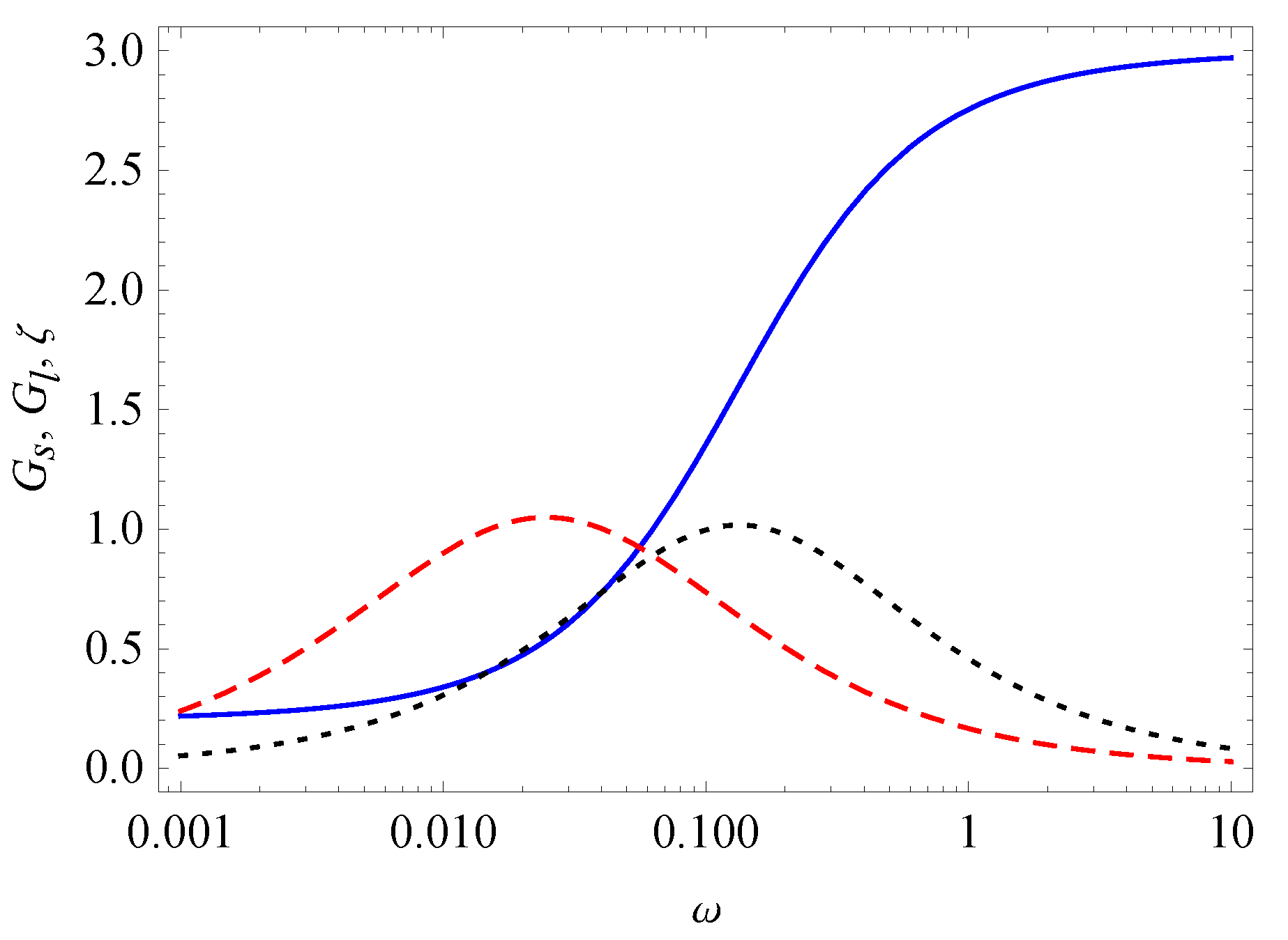
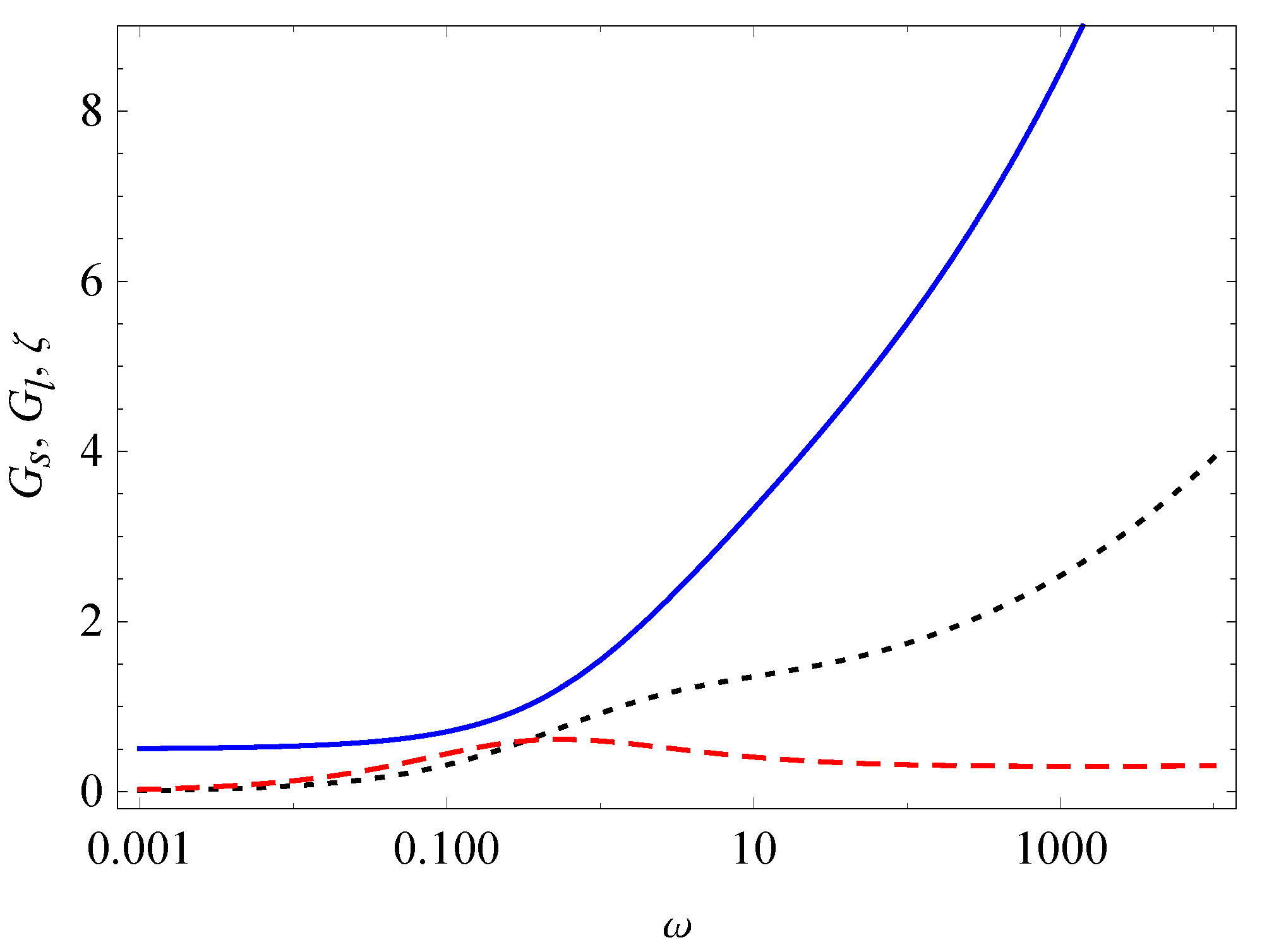
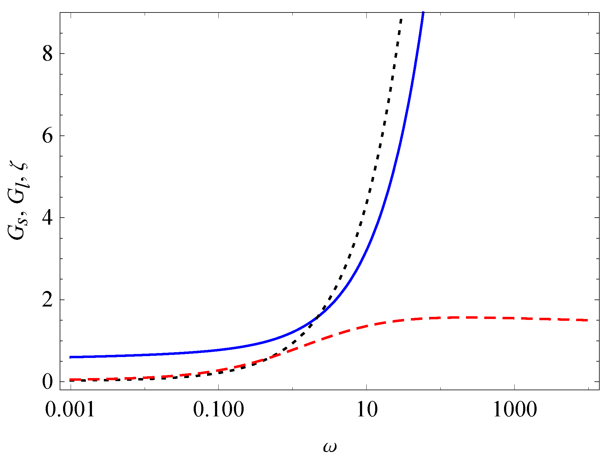
In Figure 1 and Figure 2, we plot the storage modulus, the loss modulus, and the loss factor against ω for two groups of different parameter values. In Figure 1, ζ m a x < G l m a x , while in Figure 2, ζ m a x > G l m a x .
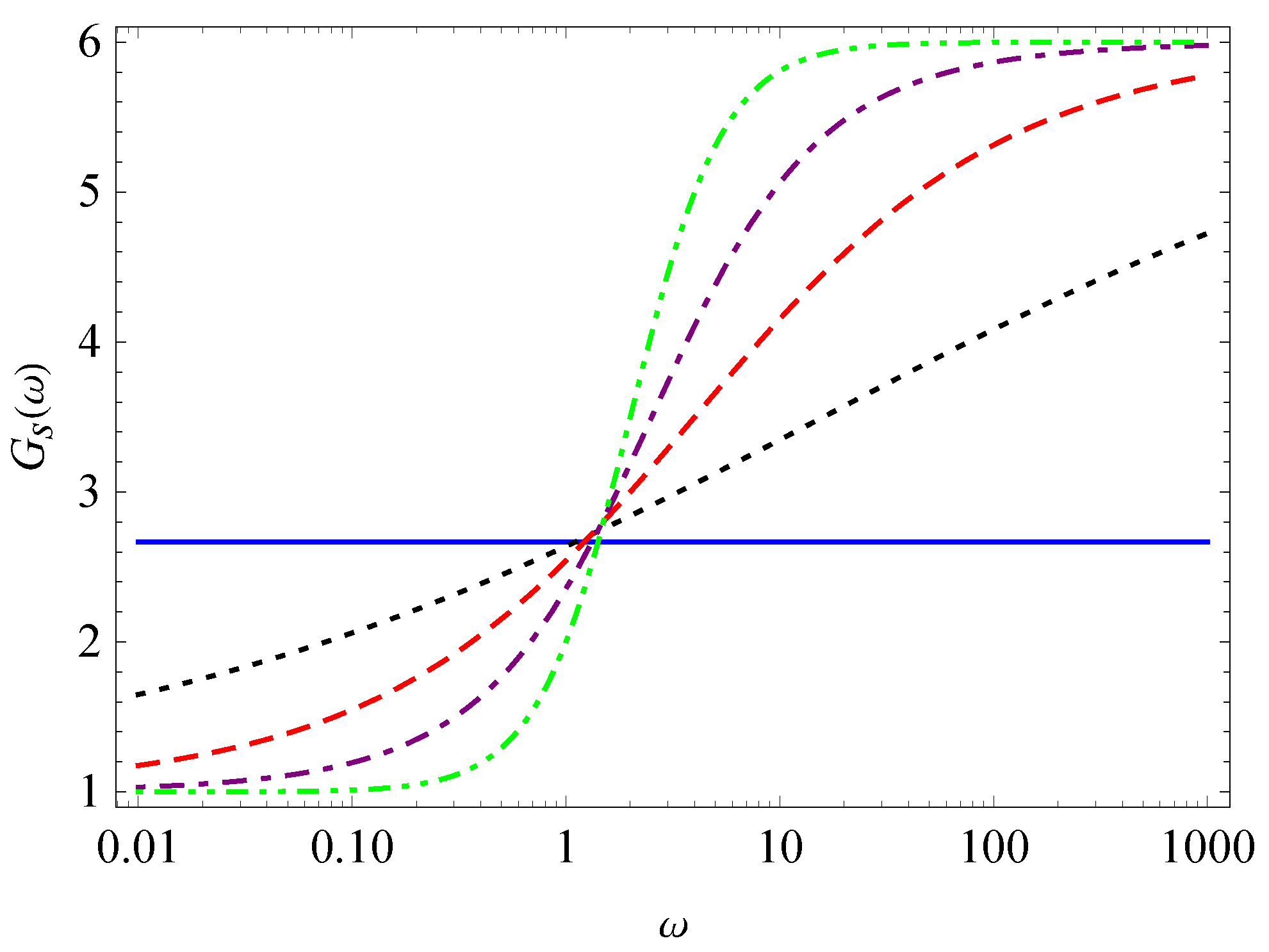
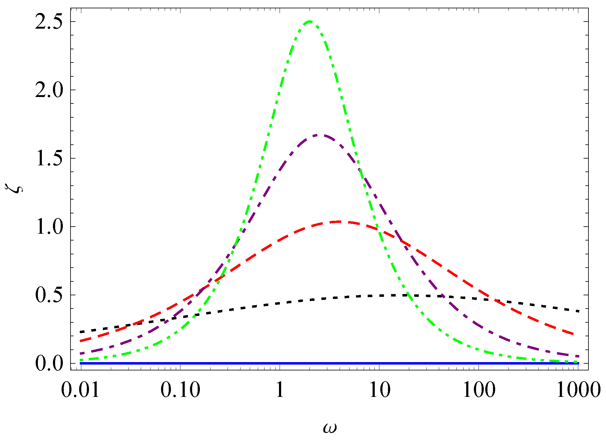
The effects in the order α on the storage modulus G s and the loss factor ζ are shown in Figure 3 and Figure 4, respectively. The increase of order α makes the curves of G s ω become steeper, but α does not affect the limits G s ( 0 ) and G s ( + ) . The increase in order α enhances the peaks of the curves of ζ ω . The plot of G l ω is similar to that of ζ ω .
The following models involve the term of the fractional derivative of order β , and we assume that α < β .
Fractional four-parameter model ( b 0 = b 1 = 0 ):
σ ( t ) + a D t α σ ( t ) = b 2 D t β ϵ ( t ) ,
G l ( ω ) = b 2 sin ( π β 2 ) ω β + a b 2 sin ( π ( β α ) 2 ) ω α + β 1 + 2 a cos ( π α 2 ) ω α + a 2 ω 2 α ,
G s ( ω ) = b 2 cos ( π β 2 ) ω β + a b 2 cos ( π ( β α ) 2 ) ω α + β 1 + 2 a cos ( π α 2 ) ω α + a 2 ω 2 α ,
ζ ( ω ) = sin ( π β 2 ) + a sin ( π ( β α ) 2 ) ω α cos ( π β 2 ) + a cos ( π ( β α ) 2 ) ω α .
By combining their derivatives, the following assertions can be yielded: G l ( ω ) and G s ( ω ) increase monotonically on [ 0 , + ) with limits
G l ( 0 ) = 0 , G l ( + ) = + ,
G s ( 0 ) = 0 , G s ( + ) = + ,
and ζ ( ω ) decreases monotonically on [ 0 , + ) with the limits
ζ ( 0 ) = tan π β 2 , ζ ( + ) = tan π ( β α ) 2 .
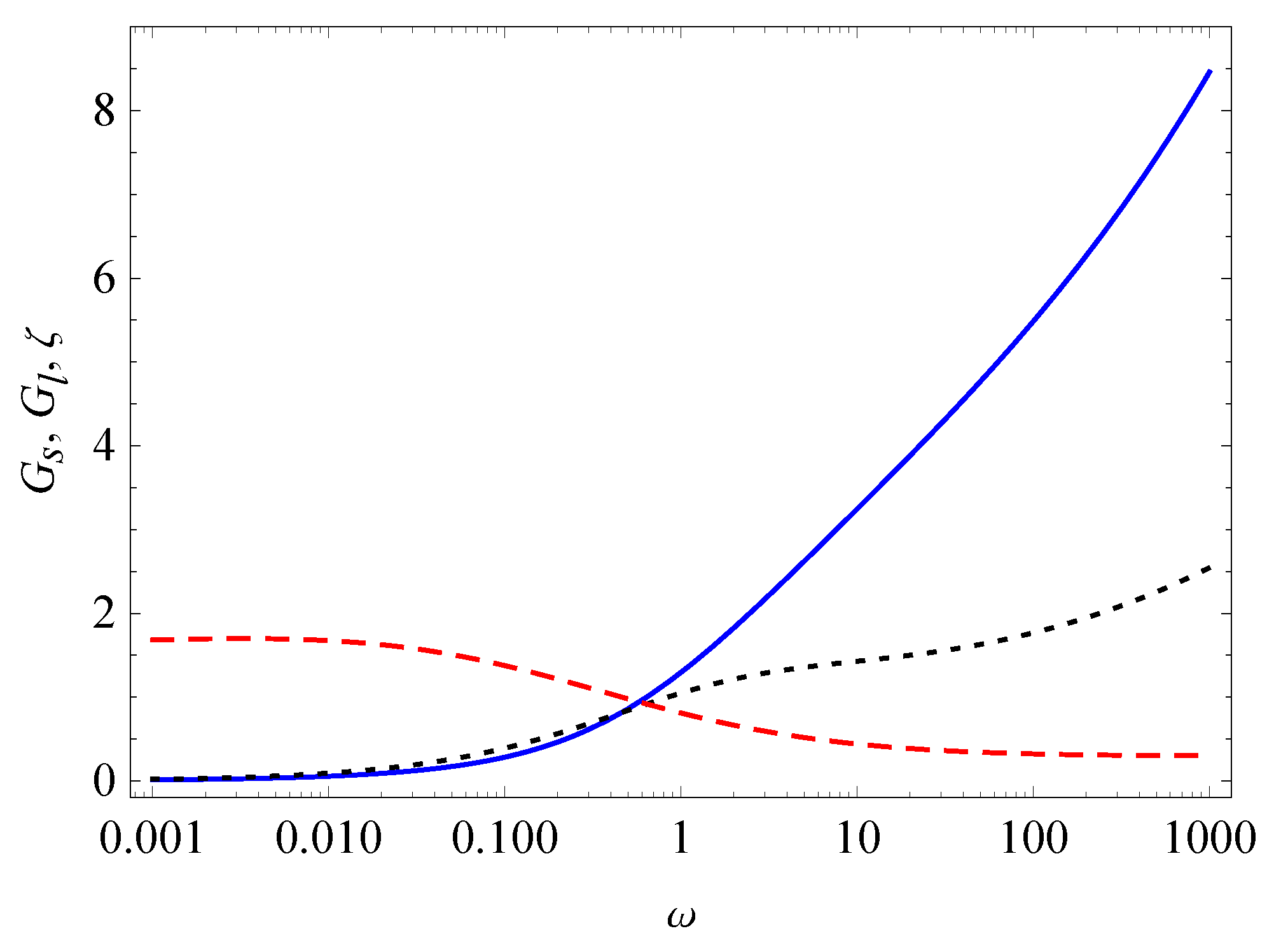
Three monotonic curves of G s , G l , and ζ versus ω are plotted in Figure 5.
Fractional five-parameter model ( b 0 = 0 ):
σ ( t ) + a D t α σ ( t ) = b 1 D t α ϵ ( t ) + b 2 D t β ϵ ( t ) ,
G l ( ω ) = b 1 sin ( π α 2 ) ω α + b 2 sin ( π β 2 ) ω β + a b 2 sin ( π ( β α ) 2 ) ω α + β 1 + 2 a cos ( π α 2 ) ω α + a 2 ω 2 α ,
G s ( ω ) = b 1 cos ( π α 2 ) ω α + b 2 cos ( π β 2 ) ω β + a b 1 ω 2 α + a b 2 cos ( π ( β α ) 2 ) ω α + β 1 + 2 a cos ( π α 2 ) ω α + a 2 ω 2 α ,
ζ ( ω ) = b 1 sin ( π α 2 ) + b 2 sin ( π β 2 ) ω β α + a b 2 sin ( π ( β α ) 2 ) ω β b 1 cos ( π α 2 ) + b 2 cos ( π β 2 ) ω β α + a b 1 ω α + a b 2 cos ( π ( β α ) 2 ) ω β .
By examining their derivatives, we can conclude that G s ( ω ) increases monotonically on [ 0 , + ) with the limits
G s ( 0 ) = 0 , G s ( + ) = + ;
G l ( ω ) satisfies G l ( 0 ) = 0 and increases monotonically to + when ω is large enough; and ζ ( ω ) satisfies
ζ ( 0 ) = tan π α 2 , ζ ( + ) = tan π ( β α ) 2 ,
and decreases monotonically when ω is large enough.
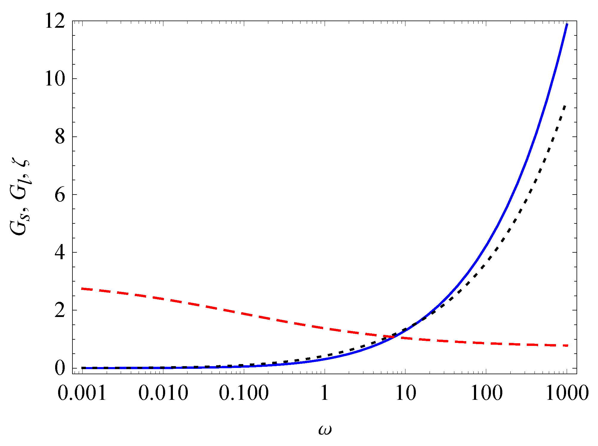
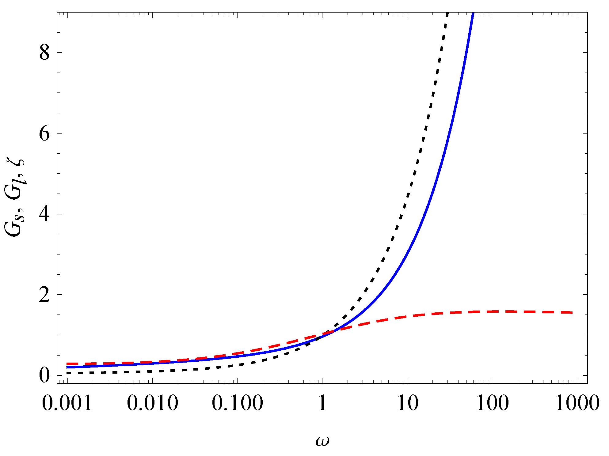
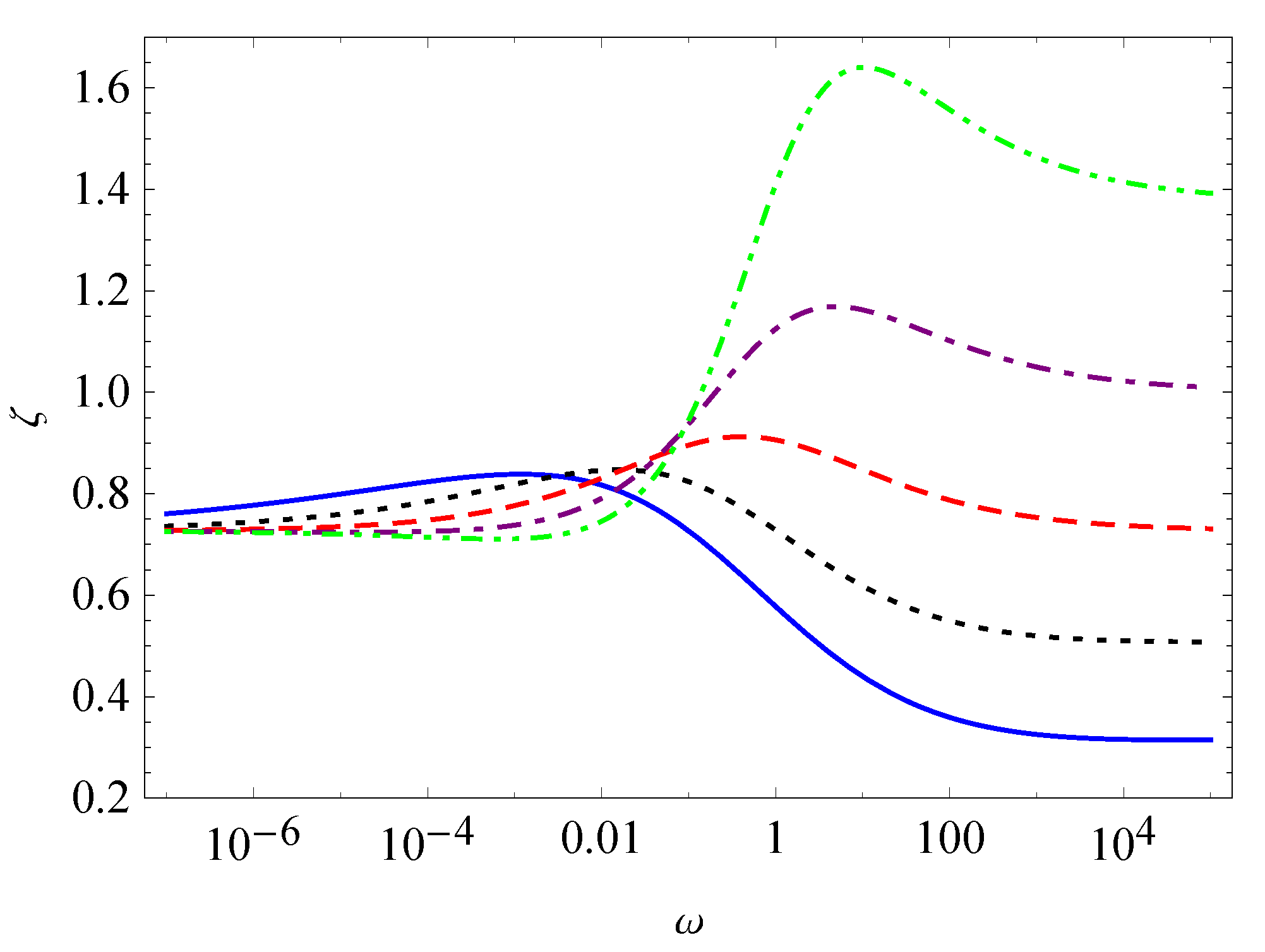
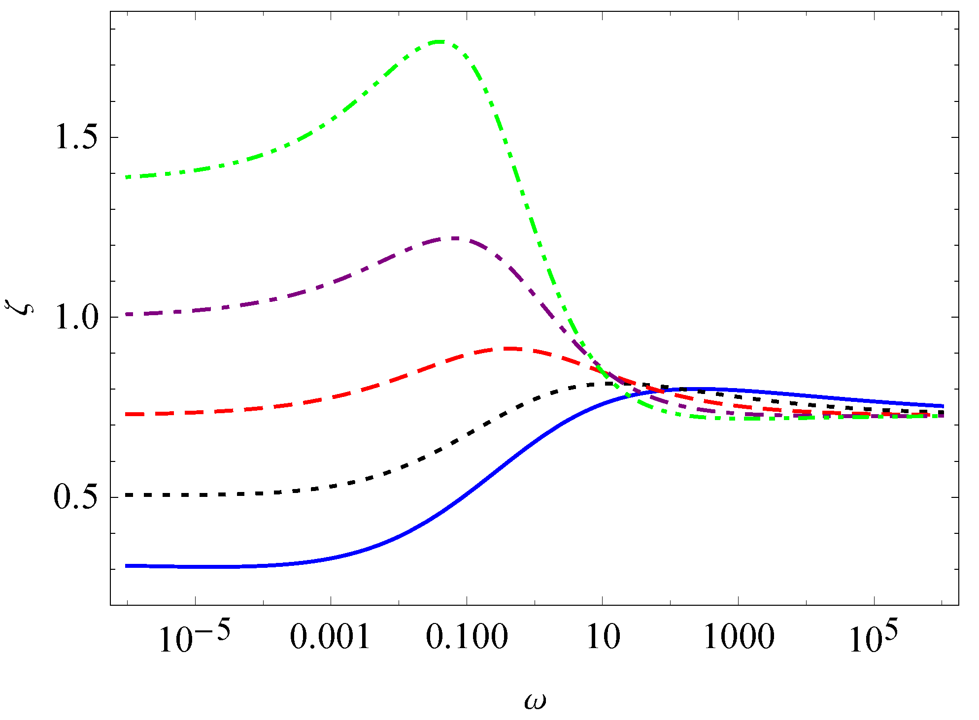
From Equation (73), the linear-logarithmic curve of ζ ω does not have symmetrical peaks if 2 α β . In Figure 6 and Figure 7, curves of G s , G l , and ζ versus ω are plotted, where the orders α and β affect the limits of ζ as ω 0 or + , but do not affect the limits of G s and G l . In order to further examine the effects of the orders α and β on the loss factor ζ , we plot the curves of ζ versus ω for different order values in Figure 8 and Figure 9. The asymmetrical peaks of the loss factor ζ are tuned by the two orders α and β .
We noticed that the two fractional derivative terms on the right-hand side of the constitutive equation lead to an asymmetrical loss factor peak. In [53], a five-parameter fractional derivative model, which also includes two fractional derivative terms with respect to the strain, but different from those of (68), was presented to describe this phenomenon.
Fractional six-parameter model (7):
By checking the signs of the derivatives, we have the following results for the general six-parameter model (7). G s ( ω ) increases monotonically on [ 0 , + ) with limits
G s ( 0 ) = b 0 , G s ( + ) = + .
G l ( ω ) satisfies G l ( 0 ) = 0 and increases monotonically to + when ω is large enough. ζ ( ω ) satisfies
ζ ( 0 ) = 0 , ζ ( + ) = tan π ( β α ) 2 .
In Figure 10 and Figure 11, curves of G s , G l , and ζ versus ω in the fractional six-parameter model (7) are plotted, where α distinctly affects the trends of ζ as ω . Compared with the fractional five-parameter model (68), here, G s ( 0 ) > 0 and ζ ( 0 ) = 0 , which are different from those in Equations (72) and (73).

3. Relaxation, Creep, and Hysteresis

The relaxation modulus and creep compliance are two important material functions describing the mechanical characteristics of viscoelastic materials. The relaxation modulus R ( t ) is the behavior of stress relaxing with time under a suddenly applied unit strain ϵ ( t ) = H ( t ) , where H ( t ) is the Heaviside unit-step function. Creep compliance C ( t ) is the strain response to an instantaneously applied stress σ ( t ) = H ( t ) . Both the material functions are nonnegative. Furthermore, for 0 < t < + , R ( t ) is decreasing and C ( t ) is increasing.
Inserting ϵ ¯ ( s ) = 1 / s into Equation (10), we obtain the relaxation modulus in the Laplace domain:
R ¯ ( s ) = b 0 + b 1 s α + b 2 s β s ( 1 + a s α ) .
If a = 0 , i.e., the model (7) degenerates into the following five-parameter model,
σ ( t ) = b 0 ϵ ( t ) + b 1 D t α ϵ ( t ) + b 2 D t β ϵ ( t ) ,
then the relaxation modulus is
R ( t ) = b 0 H ( t ) + b 1 t α Γ ( 1 α ) + b 2 t β Γ ( 1 β ) .
If a > 0 , we rewrite Equation (76) as
R ¯ ( s ) = a 1 b 0 s 1 + a 1 b 1 s α 1 + a 1 b 2 s β 1 a 1 + s α .
By Formula (6), the inverse Laplace transform yields the relaxation modulus in terms of the Mittag–Leffler functions
R ( t ) = a 1 b 0 t α E α , α + 1 ( a 1 t α ) + a 1 b 1 E α , 1 ( a 1 t α ) + a 1 b 2 t α β E α , α + 1 β ( a 1 t α ) .
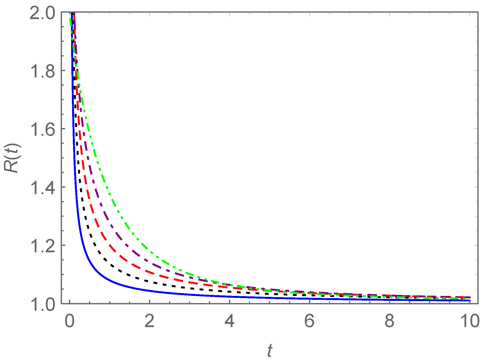
The relaxation moduli R ( t ) in Equations (78) and (80) are plotted in Figure 12 and Figure 13, respectively. The appearance of the fractional derivative term with respect to stress accelerates the relaxation of stress by comparing the two figures. In addition, the variation in the order tunes the relaxing rate.
In a similar manner, letting σ ¯ ( s ) = 1 / s in Equation (10), we obtain the creep compliance in the Laplace domain:
C ¯ ( s ) = 1 + a s α s ( b 0 + b 1 s α + b 2 s β ) .
We give the creep compliance C ( t ) by discriminating the following three cases.
Case I. 
b 2 = b 1 = 0
In this case, it is necessary that b 0 > 0 and a = 0 from the condition (8). The model degenerates into a Hook spring σ ( t ) = b 0 ϵ ( t ) , and the creep compliance is
C ( t ) = 1 b 0 H ( t ) .
In fact, there is no “creep”.
Case II. 
b 2 = 0 and b 1 0
This case corresponds to the fractional Zener model (48). Rewriting Equation (81) as
C ¯ ( s ) = 1 + a s α s ( b 0 + b 1 s α ) = s 1 + a s α 1 b 1 ( s α + b 0 b 1 ) ,
and applying the inverse Laplace transform using Formula (6), we derive the creep compliance in terms of the Mittag–Leffler functions:
C ( t ) = 1 b 1 t α E α , α + 1 ( b 0 b 1 t α ) + a b 1 E α , 1 ( b 0 b 1 t α ) .
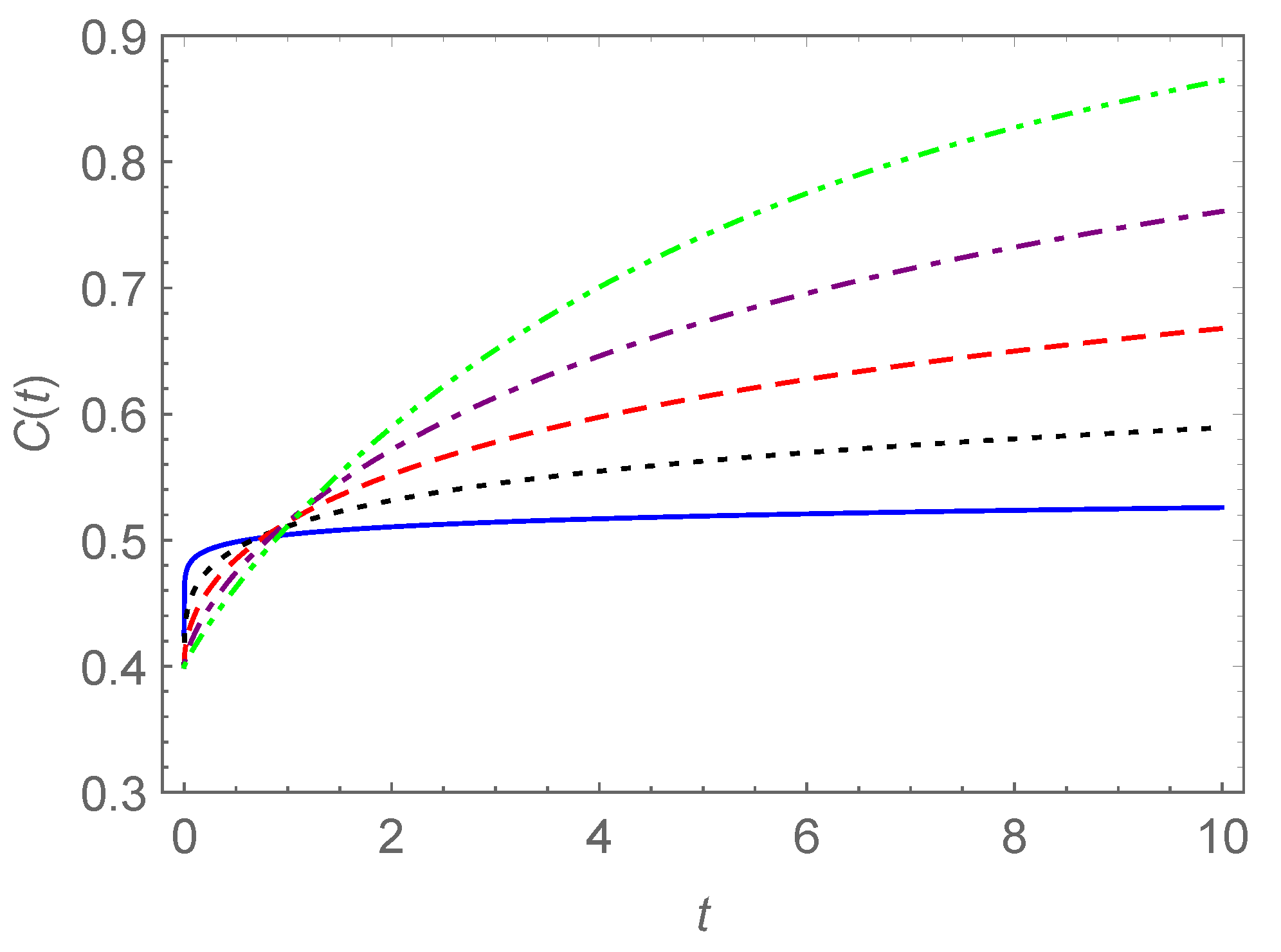
In Figure 14, the curves of the creep compliance C ( t ) in Equation (84) are plotted for different values of α . Apart from an initial period, the creep compliance C ( t ) increases with the rising α .
Case III. 
b 2 0
Rewriting Equation (81) as
C ¯ ( s ) = k = 0 ( b 0 ) k b 2 k + 1 s 1 α α k + a s 1 α k ( b 1 b 2 + s β α ) k + 1 ,
and operating the inverse Laplace transform using Formula (6), we have the creep compliance:
C ( t ) = k = 0 ( b 0 / b 2 ) k b 2 k ! t β k + β E β α , 1 + α k + β ( k ) ( b 1 b 2 t β α ) + a t α E β α , 1 + α k α + β ( k ) ( b 1 b 2 t β α ) .
Here, the creep compliance is expressed as a series in which the Mittag–Leffler functions and their derivatives are involved.
In terms of the creep compliance C ( t ) and the relaxation modulus R ( t ) , the strain and the stress have the expressions
ϵ ( t ) = C ( t ) σ ˙ ( t ) , σ ( t ) = R ( t ) ϵ ˙ ( t ) ,
respectively, where ∗ denotes the convolution.
Making use of the creep compliance C ( t ) and Formula (87), we may simulate the hysteresis phenomena. We consider the strain response to the sinusoidal stress loading σ ( t ) = sin ( t ) . From (87), the strain response is
ϵ ( t ) = C ( t ) cos ( t ) .
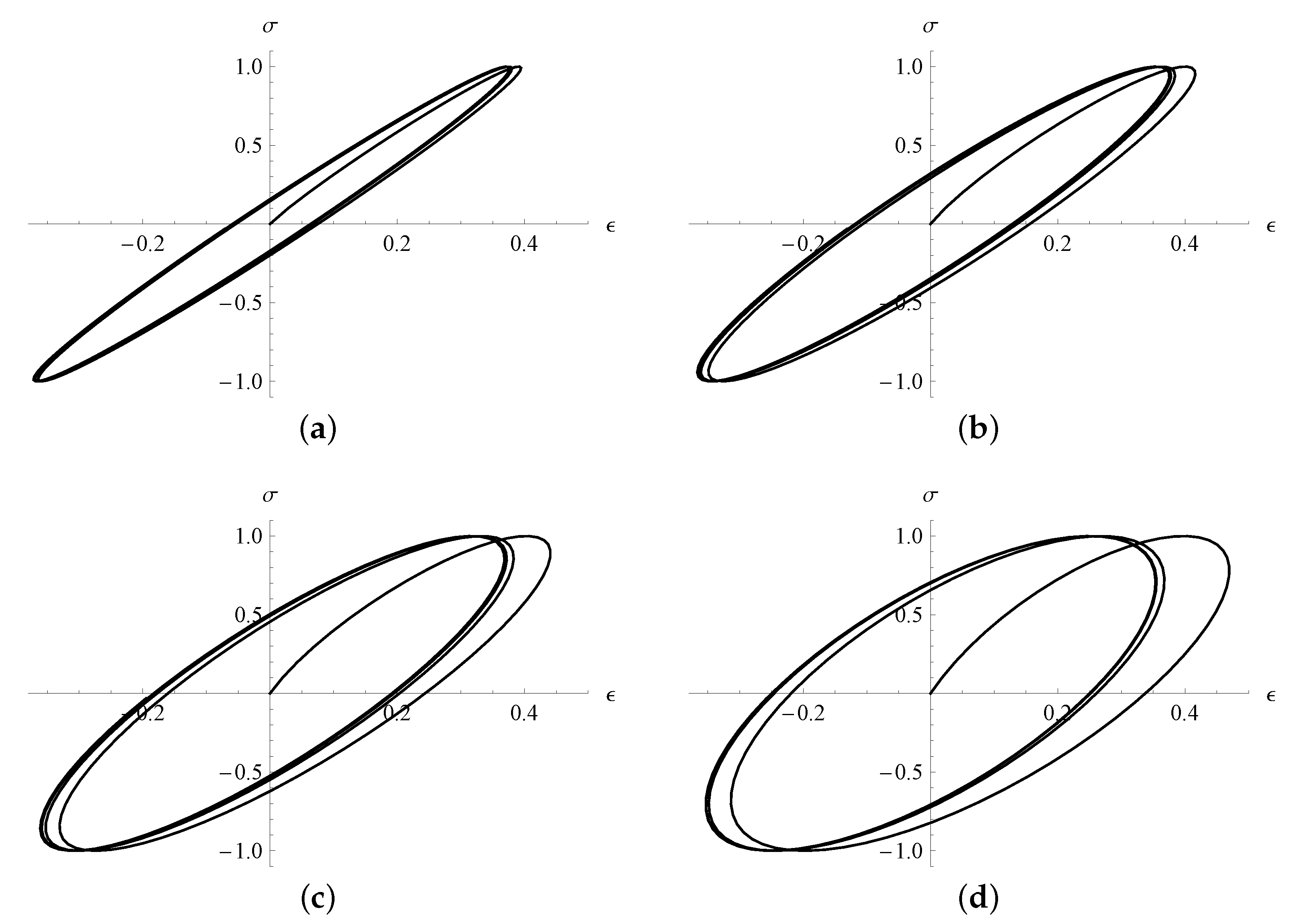
For the numerical simulation here, we use the fractional Zener model and its creep compliance in Equation (84). Taking a = 0.5 , b 0 = 1 , b 1 = 3 , and four different values of α (0.25, 0.5, 0.75, and 1), the stress–strain hysteresis loops are depicted in Figure 15, where t serves as the parameter varying from 0 to 8 π . For comparison, the coordinate ranges are the same in the four subfigures.
The unloading curve falls to the right side of the loading curve to form the hysteresis loops. In other words, the fluctuations of the strain fall behind those of the stress. With increasing α , the hysteresis loops grow fat and encircle a larger area, which means that the ability of dissipation of the model is raised.

4. Conclusions

We considered dissipation, creep, relaxation, and hysteresis resulting from a six-parameter fractional constitutive model and its particular cases. In Section 2, we considered the storage modulus, loss modulus, and loss factor, as well as their characteristics for different fractional constitutive models based on the thermodynamic requirements. We proved that for the fractional Maxwell model, the storage modulus G s increases monotonically, while the loss modulus G l has symmetrical peaks for its curve against the logarithmic scale log ( ω ) , and for the fractional Zener model, the storage modulus G s monotonically increases, while the loss modulus G l and the loss factor ζ have symmetrical peaks for their curves against the logarithmic scale log ( ω ) . The peak values and corresponding stationary points were accurately given. A series of results for the fractional Zener model were presented in Proposition 3. In Section 3, we derived the relaxation modulus and the creep compliance for the six-parameter fractional constitutive model in terms of the Mittag–Leffler functions. Then, the stress–strain hysteresis loops were simulated by making use of the derived creep compliance for the fractional Zener model. These results show that the fractional constitutive models could simulate the relaxation, creep, dissipation, and hysteresis phenomena of viscoelastic bodies, and the tuning of the fractional orders α and β could model the physical properties well.

Author Contributions

Conceptualization, J.-S.D. and Y.-Q.C.; Data curation, D.-C.H.; Formal analysis, J.-S.D. and Y.-Q.C.; Funding acquisition, J.-S.D.; Methodology, J.-S.D.; Software, D.-C.H.; Validation, J.-S.D. and Y.-Q.C.; Visualization, D.-C.H.; Writing—original draft, J.-S.D.; Writing—review and editing, J.-S.D., D.-C.H., and Y.-Q.C. All authors have read and agreed to the published version of the manuscript.

Funding

This research was funded by the National Natural Science Foundation of China (No. 11772203).

Institutional Review Board Statement

Not applicable.

Informed Consent Statement

Not applicable.

Data Availability Statement

Not applicable.

Acknowledgments

The authors show their appreciation for the valuable comments from the reviewers on the manuscript.

Conflicts of Interest

The authors declare no conflict of interest.

References

  1. Oldham, K.B.; Spanier, J. The Fractional Calculus; Academic: New York, NY, USA, 1974. [Google Scholar]
  2. Ross, B. (Ed.) Fractional Calculus and Its Applications (Lecture Notes in Mathematics 457); Springer: Berlin/Heidelberg, Germany, 1975. [Google Scholar]
  3. Gorenflo, R.; Vessella, S. Abel Integral Equations; Springer: Berlin/Heidelberg, Germany, 1991. [Google Scholar]
  4. Miller, K.S.; Ross, B. An Introduction to the Fractional Calculus and Fractional Differential Equations; Wiley: New York, NY, USA, 1993. [Google Scholar]
  5. Kiryakova, V. Generalized Fractional Calculus and Applications (Pitman Res. Notes in Math. Ser., Vol. 301); Longman Scientific & Technical and John Wiley & Sons, Inc.: Harlow, UK; New York, NY, USA, 1994. [Google Scholar]
  6. Carpinteri, A.; Mainardi, F. (Eds.) Fractals and Fractional Calculus in Continuum Mechanics; Springer: Wien, Austria; New York, NY, USA, 1997. [Google Scholar]
  7. Podlubny, I. Fractional Differential Equations; Academic: San Diego, CA, USA, 1999. [Google Scholar]
  8. Kilbas, A.A.; Srivastava, H.M.; Trujillo, J.J. Theory and Applications of Fractional Differential Equations; Elsevier: Amsterdam, The Netherlands, 2006. [Google Scholar]
  9. Mainardi, F. Fractional Calculus and Waves in Linear Viscoelasticity; Imperial College: London, UK, 2010. [Google Scholar]
  10. Diethelm, K. The Analysis of Fractional Differential Equations; Springer: Berlin/Heidelberg, Germany, 2010. [Google Scholar]
  11. Monje, C.A.; Chen, Y.Q.; Vinagre, B.M.; Xue, D.; Feliu, V. Fractional-Order Systems and Controls, Fundamentals and Applications; Springer: London, UK, 2010. [Google Scholar]
  12. Klafter, J.; Lim, S.C.; Metzler, R. (Eds.) Fractional Dynamics: Recent Advances; World Scientific: Singapore, 2011. [Google Scholar]
  13. Băleanu, D.; Diethelm, K.; Scalas, E.; Trujillo, J.J. Fractional Calculus Models and Numerical Methods. Series on Complexity, Nonlinearity and Chaos; World Scientific: Boston, MA, USA, 2012. [Google Scholar]
  14. Jiao, Z.; Chen, Y.; Podlubny, I. Distributed-Order Dynamic Systems–Stability, Simulation, Applications and Perspectives; Springer: London, UK, 2012. [Google Scholar]
  15. Li, C.; Zeng, F. Numerical Methods for Fractional Calculus; CRC Press: Boca Raton, FL, USA, 2015. [Google Scholar]
  16. Scott-Blair, G.W. The role of psychophysics in rheology. J. Colloid Sci. 1947, 2, 21–32. [Google Scholar] [CrossRef]
  17. Tan, W.; Xu, M. Plane surface suddenly set in motion in a viscoelastic fluid with fractional Maxwell model. Acta Mech. Sin. 2002, 18, 342–349. [Google Scholar]
  18. Yang, P.; Lam, Y.C.; Zhu, K.Q. Constitutive equation with fractional derivatives for the generalized UCM model. J. Non-Newton. Fluid Mech. 2010, 165, 88–97. [Google Scholar] [CrossRef]
  19. Wang, X.; Xu, H.; Qi, H. Numerical analysis for rotating electro-osmotic flow of fractional Maxwell fluids. Appl. Math. Lett. 2020, 103, No. 106179. [Google Scholar] [CrossRef]
  20. Gerasimov, A.N. A generalization of linear laws of deformation and its application to inner friction problems. Prikl. Mat. Mekh. 1948, 12, 251–259. [Google Scholar]
  21. Koeller, R.C. Applications of fractional calculus to the theory of viscoelasticity. J. Appl. Mech. 1984, 51, 299–307. [Google Scholar] [CrossRef]
  22. Koeller, R.C. Polynomial operators, Stieltjes convolution, and fractional calculus in hereditary mechanics. Acta Mech. 1986, 58, 251–264. [Google Scholar] [CrossRef]
  23. Schiessel, H.; Metzler, R.; Blumen, A.; Nonnenmacher, T.F. Generalized viscoelastic models: Their fractional equations with solutions. J. Phys. A Math. Gen. 1995, 28, 6567–6584. [Google Scholar] [CrossRef]
  24. Nigmatullin, R.R. The realization of the generalized transfer equation in a medium with fractal geometry. Phys. Stat. Sol. B 1986, 133, 425–430. [Google Scholar] [CrossRef]
  25. Schneider, W.R.; Wyss, W. Fractional diffusion and wave equations. J. Math. Phys. 1989, 30, 134–144. [Google Scholar] [CrossRef]
  26. Metzler, R.; Glockle, W.G.; Nonnenmacher, T.F. Fractional model equation for anomalous diffusion. Physica A 1994, 211, 13–24. [Google Scholar] [CrossRef]
  27. Metzler, R.; Klafter, J. The random walk’s guide to anomalous diffusion: A fractional dynamics approach. Phys. Rep. 2000, 339, 1–77. [Google Scholar] [CrossRef]
  28. Duan, J.S.; Xu, M.Y. Concentration distribution of fractional anomalous diffusion caused by an instantaneous point source. Appl. Math. Mech. (Engl. Ed.) 2003, 24, 1302–1308. [Google Scholar]
  29. Jiang, X.; Xu, M.; Qi, H. The fractional diffusion model with an absorption term and modified Fick’s law for non-local transport processes. Nonlinear Anal. Real World Appl. 2010, 11, 262–269. [Google Scholar] [CrossRef]
  30. Qi, H.; Jiang, X. Solutions of the space-time fractional Cattaneo diffusion equation. Physica A 2011, 390, 1876–1883. [Google Scholar] [CrossRef]
  31. Bagley, R.L.; Calico, R.A. Fractional order state equations for the control of viscoelastically damped structures. J. Guid. Control Dyn. 1991, 14, 304–311. [Google Scholar] [CrossRef]
  32. Makroglou, A.; Miller, R.K.; Skaar, S. Computational results for a feedback control for a rotating viscoelastic beam. J. Guid. Control Dyn. 1994, 17, 84–90. [Google Scholar] [CrossRef]
  33. Chen, Y.; Moore, K.L. Analytical stability bound for a class of delayed fractional-order dynamic systems. Nonlinear Dyn. 2002, 29, 191–200. [Google Scholar] [CrossRef]
  34. Chen, Y.Q.; Xue, D.; Dou, H. Fractional calculus and biomimetic control. In Proceedings of the 2004 IEEE International Conference on Robotics and Biomimetics, Shengyang, China, 22–25 August 2004; pp. 901–906. [Google Scholar]
  35. Li, Y.; Chen, Y.Q.; Podlubny, I. Mittag-Leffler stability of fractional order nonlinear dynamic systems. Automatica 2009, 45, 1965–1969. [Google Scholar] [CrossRef]
  36. Ding, C.; Cao, J.; Chen, Y.Q. Fractional-order model and experimental verification for broadband hysteresis in piezoelectric actuators. Nonlinear Dyn. 2019, 98, 3143–3153. [Google Scholar] [CrossRef]
  37. Sokolov, I.M.; Klafter, J.; Blumen, A. Fractional kinetics. Phys. Today 2002, 55, 48–54. [Google Scholar] [CrossRef]
  38. Li, C.P.; Deng, W.H.; Xu, D. Chaos synchronization of the Chua system with a fractional order. Physica A 2006, 360, 171–185. [Google Scholar] [CrossRef]
  39. Wang, Z.H.; Hu, H.Y. Stability of a linear oscillator with damping force of the fractional-order derivative. Sci. China Ser. G 2010, 53, 345–352. [Google Scholar] [CrossRef]
  40. Li, C.; Ma, Y. Fractional dynamical system and its linearization theorem. Nonlinear Dyn. 2013, 71, 621–633. [Google Scholar] [CrossRef]
  41. Wu, G.C.; Baleanu, D.; Xie, H.P.; Chen, F.L. Chaos synchronization of fractional chaotic maps based on the stability condition. Physica A 2016, 460, 374–383. [Google Scholar] [CrossRef]
  42. Scott-Blair, G.W. Analytical and integrative aspects of the stress-strain-time problem. J. Sci. Instrum. 1944, 21, 80–84. [Google Scholar] [CrossRef]
  43. Scott-Blair, G.W. Survey of General and Applied Rheology; Pitman: London, UK, 1949. [Google Scholar]
  44. Bland, D.R. The Theory of Linear Viscoelasticity; Pergamon: Oxford, UK, 1960. [Google Scholar]
  45. Bagley, R.L.; Torvik, P.J. A theoretical basis for the application of fractional calculus to viscoelasticity. J. Rheol. 1983, 27, 201–210. [Google Scholar] [CrossRef]
  46. Rogers, L. Operators and fractiorial derivatives for viscoelastic constituitive equations. J. Rheol. 1983, 27, 351–372. [Google Scholar] [CrossRef]
  47. Pritz, T. Analysis of four-parameter fractional derivative model of real solid materials. J. Sound Vib. 1996, 195, 103–115. [Google Scholar] [CrossRef]
  48. Mainardi, F.; Spada, G. Creep, relaxation and viscosity properties for basic fractional models in rheology. Eur. Phys. J. Spec. Top. 2011, 193, 133–160. [Google Scholar] [CrossRef] [Green Version]
  49. Atanacković, T.M.; Pilipović, S.; Stanković, B.; Zorica, D. Fractional Calculus with Applications in Mechanics; Wiley: New York, NY, USA, 2014. [Google Scholar]
  50. Duan, J.S.; Qiu, X. The periodic solution of Stokes’ second problem for viscoelastic fluids as characterized by a fractional constitutive equation. J. Non-Newton. Fluid Mech. 2014, 205, 11–15. [Google Scholar] [CrossRef]
  51. Lewandowski, R.; Chorazyczewski, B. Identification of the parameters of the Kelvin-Voigt and the Maxwell fractional models, used to modeling of viscoelastic dampers. Comput. Struct. 2010, 88, 1–17. [Google Scholar] [CrossRef]
  52. Friedrich, C. Mechanical stress relaxation in polymers: Fractional integral model versus fractional differential model. J. Non-Newton. Fluid Mech. 1993, 46, 307–314. [Google Scholar] [CrossRef]
  53. Pritz, T. Five-parameter fractional derivative model for polymeric dampling materials. J. Sound Vib. 2003, 265, 935–952. [Google Scholar] [CrossRef]
  54. Yang, S.M.; Duan, J.S. Response analysis of six-parameter fractional constitutive model. Phys. Scr. 2021, 96, 025220. [Google Scholar] [CrossRef]
  55. Colombaro, I.; Giusti, A.; Vitali, S. Storage and dissipation of energy in Prabhakar viscoelasticity. Mathematics 2018, 6, 15. [Google Scholar] [CrossRef] [Green Version]
  56. Caputo, M. Distributed order differential equations modelling dielectric induction and diffusion. Fract. Calc. Appl. Anal. 2001, 4, 421–442. [Google Scholar]
  57. Duan, J.S.; Chen, Y.Q. Mechanical response and simulation for constitutive equations with distributed order derivatives. Int. J. Model. Simul. Sci. Comput. 2017, 8, 1750040. [Google Scholar] [CrossRef] [Green Version]
  58. Duan, J.S.; Qiu, X. Stokes’ second problem of viscoelastic fluids with constitutive equation of distributed-order derivative. Appl. Math. Comput. 2018, 331, 130–139. [Google Scholar] [CrossRef]
  59. Duan, J.S.; Chen, L. Oscillatory shear flow between two parallel plates for viscoelastic constitutive model of distributed-order derivative. Int. J. Numer. Methods Heat Fluid Flow 2020, 30, 1137–1148. [Google Scholar] [CrossRef]
  60. Mainardi, F.; Gorenflo, R. On Mittag-Leffler-type functions in fractional evolution processes. J. Comput. Appl. Math. 2000, 118, 283–299. [Google Scholar] [CrossRef] [Green Version]
  61. Gorenflo, R.; Kilbas, A.A.; Mainardi, F.; Rogosin, S. Mittag-Leffler Functions, Related Topics and Applications, 2nd ed.; Springer: Berlin/Heidelberg, Germany, 2020. [Google Scholar]
  62. Deng, L.; Seethaler, R.J.; Chen, Y.Q.; Yang, P.; Cheng, Q. Modified Elman neural network based neural adaptive inverse control of rate-dependent hysteresis. In Proceedings of the 2016 International Joint Conference on Neural Networks (IJCNN), Vancouver, BC, Canada, 24–29 July 2016; pp. 2366–2373. [Google Scholar]
  63. Li, Z.; Zeng, J.; Chen, Y.; Ma, G.; Liu, G. Adaptive control of a piezo-positioning mechanism with hysteresis and input saturation using time delay estimation. IEEE Access 2020, 8, 176062–176072. [Google Scholar] [CrossRef]
  64. Pei, J.S.; Carboni, B.; Lacarbonara, W. Mem-models as building blocks for simulation and identification of hysteretic systems. Nonlinear Dyn. 2020, 100, 973–998. [Google Scholar] [CrossRef]
  65. Bagley, R.L.; Torvik, P.J. On the fractional calculus model of viscoelastic behavior. J. Rheol. 1986, 30, 133–155. [Google Scholar] [CrossRef]
  66. Palade, L.I.; Verney, V.; Attané, P. A modified fractional model to describe the entire viscoelastic behavior of polybutadienes from flow to glassy regime. Rheol. Acta 1996, 35, 265–273. [Google Scholar] [CrossRef]
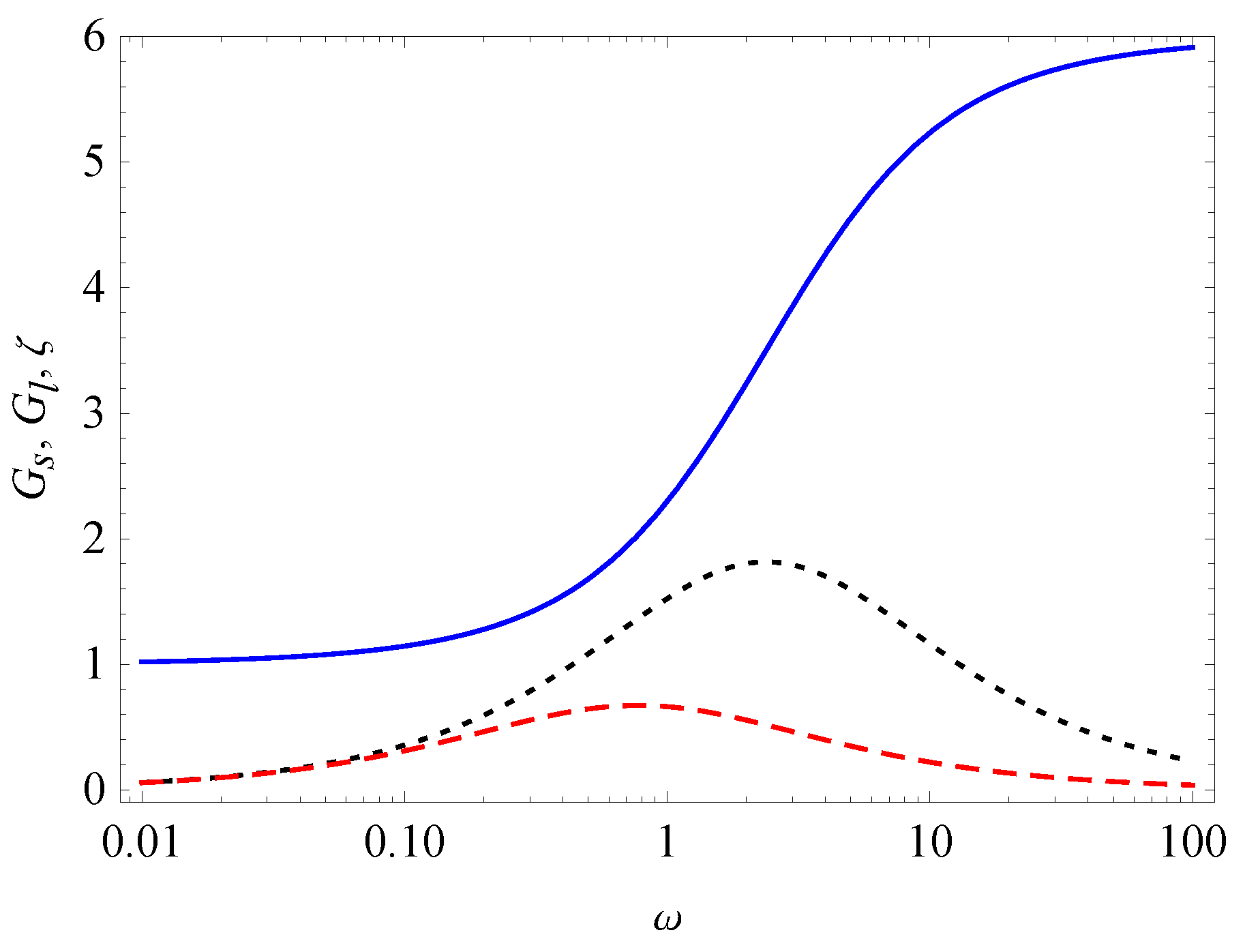
Figure 1. Curves of G s (solid line), G l (dotted line), and ζ (dashed line) versus ω for a = 0.5 , b 0 = 1 , b 1 = 3 , and α = 0.8 in the fractional Zener model (48).
Fractalfract 05 00036 g001
Figure 2. Curves of G s (solid line), G l (dotted line), and ζ (dashed line) versus ω for a = 5 , b 0 = 0.2 , b 1 = 15 , and α = 0.8 in the fractional Zener model (48).
Fractalfract 05 00036 g002
Figure 3. Curves of G s ω for a = 0.5 , b 0 = 1 , and b 1 = 3 and for α = 0 (solid line), 0.25 (dotted line), 0.5 (dashed line), 0.75 (dotted–dashed line), and 1 (dotted–dotted–dashed line) in the fractional Zener model (48).
Fractalfract 05 00036 g003
Figure 4. Curves of ζ ω for a = 0.5 , b 0 = 1 , and b 1 = 3 and for α = 0 (solid line), 0.25 (dotted line), 0.5 (dashed line), 0.75 (dotted–dash line), and 1 (dotted–dotted–dashed line) in the fractional Zener model (48).
Fractalfract 05 00036 g004
Figure 5. Curves of G s (solid line), G l (dotted line), and ζ (dashed line) versus ω for a = 1 , b 2 = 1 , α = 0.4 , and β = 0.8 in the fractional four-parameter model (61).
Fractalfract 05 00036 g005
Figure 6. Curves of G s (solid line), G l (dotted line), and ζ (dashed line) versus ω for a = 1 , b 1 = 1 , b 2 = 2 , α = 0.6 , and β = 0.8 in the fractional five-parameter model (68).
Fractalfract 05 00036 g006
Figure 7. Curves of G s (solid line), G l (dotted line), and ζ (dashed line) versus ω for a = 1 , b 1 = 1 , b 2 = 2 , α = 0.2 , and β = 0.8 in the fractional five-parameter model (68).
Fractalfract 05 00036 g007
Figure 8. Curves of ζ ω for a = 1 , b 1 = 1 , b 2 = 2 , and α = 0.4 and for β = 0.6 (solid line), 0.7 (dotted line), 0.8 (dashed line), 0.9 (dotted–dashed line), and 1 (dotted–dotted–dashed line) in the fractional five-parameter model (68).
Fractalfract 05 00036 g008
Figure 9. Curves of ζ ω for a = 1 , b 1 = 1 , b 2 = 2 , and β α = 0.4 and for α = 0.2 (solid line), 0.3 (dotted line), 0.4 (dashed line), 0.5 (dotted–dashed line), and 0.6 (dotted–dotted–dashed line) in the fractional five-parameter model (68).
Fractalfract 05 00036 g009
Figure 10. Curves of G s (solid line), G l (dotted line), and ζ (dashed line) versus ω for a = 1 , b 0 = 0.5 , b 1 = 1 , b 2 = 2 , α = 0.6 , and β = 0.8 in the fractional six-parameter model (7).
Fractalfract 05 00036 g010
Figure 11. Curves of G s (solid line), G l (dotted line), and ζ (dashed line) versus ω for a = 1 , b 0 = 0.5 , b 1 = 1 , b 2 = 2 , α = 0.2 , and β = 0.8 in the fractional six-parameter model (7).
Fractalfract 05 00036 g011
Figure 12. Curves of the relaxation modulus R ( t ) in Equation (78) for b 0 = b 1 = b 2 = 1 , β = 0.9 , and α = 0.1 (solid line), 0.3 (dotted line), 0.5 (dashed line), 0.7 (dotted–dashed line), and 0.9 (dotted–dotted–dashed line).
Fractalfract 05 00036 g012
Figure 13. Curves of the relaxation modulus R ( t ) in Equation (80) for a = b 0 = b 1 = b 2 = 1 , β = 0.9 , and α = 0.1 (solid line), 0.3 (dotted line), 0.5 (dashed line), 0.7 (dotted–dashed line), and 0.9 (dotted–dotted–dashed line).
Fractalfract 05 00036 g013
Figure 14. Curves of the creep compliance C ( t ) in Equation (84) for a = 2 , b 0 = 1 , b 1 = 5 , and α = 0.1 (solid line), 0.3 (dotted line), 0.5 (dashed line), 0.7 (dotted–dashed line), and 0.9 (dotted–dotted–dashed line).
Fractalfract 05 00036 g014
Figure 15. Stress–strain hysteresis loops for a = 0.5 , b 0 = 1 , and b 1 = 3 and for α = 0.25 (a), 0.5 (b), 0.75 (c), and 1 (d) in the fractional Zener model.
Fractalfract 05 00036 g015
Publisher’s Note: MDPI stays neutral with regard to jurisdictional claims in published maps and institutional affiliations.