The Impact of Anomalous Diffusion on Action Potentials in Myelinated Neurons

Abstract

Action potentials in myelinated neurons happen only at specialized locations of the axons known as the nodes of Ranvier. The shapes, timings, and propagation speeds of these action potentials are controlled by biochemical interactions among neurons, glial cells, and the extracellular space. The complexity of brain structure and processes suggests that anomalous diffusion could affect the propagation of action potentials. In this paper, a spatio-temporal fractional cable equation for action potentials propagation in myelinated neurons is proposed. The impact of the ionic anomalous diffusion on the distribution of the membrane potential is investigated using numerical simulations. The results show spatially narrower action potentials at the nodes of Ranvier when using spatial derivatives of the fractional order only and delayed or lack of action potentials when adding a temporal derivative of the fractional order. These findings could reveal the pathological patterns of brain diseases such as epilepsy, multiple sclerosis, and Alzheimer’s disease, which have become more prevalent in the latest years.

1. Introduction

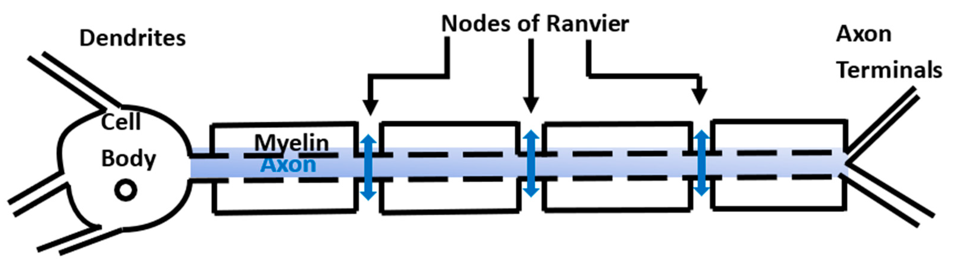
Myelination of neurons is a critical growth process taking place during the first two years of life, which facilitates the fast transmission of information throughout the body. The process involves the wrapping of the neuronal axons by myelin sheaths made of multiple layers of glial plasma membrane. The myelinated regions are separated by the nodes of Ranvier (Figure 1). Some specialized glial cells called oligodendrocytes produce myelin and create the neuro–glial-controlled clustering of voltage-gated sodium channels at the nodes of Ranvier and the aggregation of fast voltage-gated potassium channels in the myelin sheath [1,2]. The existence of some slow potassium channels in the nodes of Ranvier was reported in [3]. Experiments performed in cell cultures and in vivo reveal that nodal-like groups are created just before the myelination starts [4]. This indicates that myelination is highly dependent on timing and neuronal surroundings, especially the amounts of certain chemicals and water. An impediment to the myelination process or damage to the myelin sheath, which may or may not lead to demyelination, could cause serious, possibly life-threatening, neurologic disorders. For instance, multiple sclerosis is the most common demyelinating disorder affecting young adults that currently has no cure [5]. Mathematical models can provide essential insights into myelination/demyelination processes that can further inspire better diagnostic and therapeutic procedures for various neurological disorders.

Neurons transmit information throughout the body via action potentials. In a myelinated neuron an action potential happens when sodium flows inside the neuron at the node of Ranvier, and potassium is released into the extracellular space between the axon and the myelin (the periaxonal space). To prevent the accumulation of potassium and osmotically driven water in the periaxonal space, potassium diffuses through the myelin’s potassium channels and the gap junctions connecting the myelin layers and is removed by the astrocyte endfeet that form gap junctions with the outermost myelin layer [6]. Thus, in myelinated neurons, the action potentials do not propagate within the axons but happen only at the nodes of Ranvier (Figure 1). The work hypothesis of this paper is that the anomalous diffusion of ions through the neuronal membrane at the nodes of Ranvier and outside the neurons can influence the propagation of action potentials.

It was observed experimentally that the voltage-gated potassium channel Kv2.1 in the plasma membrane of a cultured human embryotic kidney cell displays anomalous diffusion [7]. Because the Kv2.1 channel shows similar clustering patterns in the membranes of cultured human embryonic kidney cells and native neurons [7], it is possible that anomalous diffusion of potassium can happen in the myelin sheath of neurons as well. The crowdedness of the very narrow ion channels [8] could be the cause of the anomalous diffusion of ions through the membrane’s channels. Anomalous diffusion of ions that could affect the propagation of action potentials does not happen only through the ion channels of the neuronal membrane. According to [4], clusters of cytoskeletal scaffolding proteins, cell-adhesion molecules, and parts of the extracellular matrix (ECM) can be found near the nodes of Ranvier, which could influence ion flow. Furthermore, anomalous diffusion of ions through the extracellular space (ECS) is also possible due to (1) the ECS geometry; (2) dead spaces of the ECS, voids, or glial wrapping around cells; (3) flow obstruction by the ECM; (4) binding sites on the cell membranes of the ECM; (5) the presence of fixed negative charges on the ECM [9] that control ion mobility [10]; and (6) the tight control of the ion and water movement in the ECS by astrocytes [6,11]. In particular, anomalous diffusion might be involved in the regulation of the extracellular potassium concentration by astrocytes, which is essential for the proper creation and propagation of action potentials (for example, an unregulated elevated extracellular potassium concentration can cause an epileptic seizure [12]). Thus, anomalous diffusion of ions and water in the vicinity of the nodes of Ranvier is caused by a combination of structural geometry and highly dynamic and possibly emerging biochemical processes.

Anomalous diffusion through various materials has been successfully modeled using fractional calculus [13]. A few generalizations of the classic cable equation that models the spatio-temporal propagation of action potentials in neurons that involve fractional derivatives have been proposed in the literature. In [14,15], a fractional cable equation was proposed that uses a temporal Riemann–Liouville fractional derivative acting on the classic Laplace operator to model anomalous electro-diffusion in neurons. In [16], a space-fractional cable equation was derived to model the non-local forward (from the neuronal body to the axon terminals) propagation of action potentials in mature myelinated neurons. In this paper, a spatio-temporal fractional cable equation is proposed that involves both spatial and temporal fractional derivatives. The equation models the bidirectional (forward and backward) propagation of the action potentials in the presence of anomalous diffusion. The proposed work is a straightforward generalization of the mathematical model in [16]. In the case when the order of the temporal derivative is 1 and only the forward propagation of the action potentials is considered, the results presented in [16] are recovered. The proposed equation is coupled with the fractional Hodgkin–Huxley equations (a slight variation of those proposed in [17]) and solved numerically using the methods in [18,19]. Computer simulations show spatially narrower action potentials at the nodes of Ranvier at a fixed time when using spatial derivatives of the fractional order only and delayed or lack of action potentials when also using a temporal derivative of the fractional order. The spatially narrower shape of the action potentials resembles the experimentally observed action potentials [20] better than the shape predicted by the classic cable equation. Delayed or lack of action potentials bear the mark of neurological disorders [21,22,23,24,25,26]. It is important to notice that these signs of brain pathology were obtained without adding many more equations and parameters to the cable equation, which is the current mathematical modeling approach.

The structure of the paper is as follows. The mathematical preliminaries needed in the paper are given in Section 2. The derivation of the spatio-temporal fractional cable equation is presented in Section 3, together with a numerical solution to the equation coupled with the fractional Hodgkin–Huxley equations. Numerical simulations are shown in Section 4. The paper ends with a section of conclusions and further work.

2. Mathematical Preliminaries

The fractional calculus results needed in the paper are given in this section [27,28,29,30,31,32].

Definition 1.

1. 

[28] (p. 33); [29]: Let$f\in L^1\left(a,b\right)$and$\alpha >0$. The left-sided Riemann–Liouville fractional integral of order$\alpha$is

$$I_{a+}^{\alpha }f\left(x\right)=\frac{1}{\mathsf{\Gamma }\left(\alpha \right)}\underset{a}{\overset{x}{{\displaystyle \int }}}\frac{f\left(y\right)}{{\left(x-y\right)}^{1-\alpha }}dy$$

(1)

and the right-sided Riemann–Liouville fractional integral of order$\alpha$is

$$I_{b-}^{\alpha }f\left(x\right)=\frac{1}{\mathsf{\Gamma }\left(\alpha \right)}\underset{x}{\overset{b}{{\displaystyle \int }}}\frac{f\left(y\right)}{{\left(y-x\right)}^{1-\alpha }}dy$$

(2)

where$\mathsf{\Gamma }\left(s\right)={{\displaystyle \int }}_0^{\infty }{t}^{s-1}{e}^{-t}dt$is the gamma function. In particular,$I_{a+}^{0}f\left(x\right)=I_{b-}^{0}f\left(x\right)=f\left(x\right).$

2. 

[27,29,31]: If$f:\left[a,b\right]\to \mathbf{R}$is$n$-times differentiable on$\left(a,b\right)\subset \mathbf{R}$with$f^{\left(n\right)}\in L^1\left(a,b\right)$and$n-1<\alpha <n, n=1,2,3\dots$, then the left-sided Caputo fractional derivative of order$\alpha$ is

$$D_{a+}^{\alpha }f\left(x\right)=\frac{1}{\mathsf{\Gamma }\left(n-\alpha \right)}\underset{a}{\overset{x}{{\displaystyle \int }}}\frac{f^{\left(n\right)}\left(y\right)}{{\left(x-y\right)}^{\alpha +1-n}}dy=I_{a+}^{n-\alpha }{f}^{\left(n\right)}\left(x\right)$$

(3)

and the right-sided Caputo fractional derivative of order $\alpha$ is

$$D_{b-}^{\alpha }f\left(x\right)=\frac{{\left(-1\right)}^n}{\mathsf{\Gamma }\left(n-\alpha \right)}\underset{x}{\overset{b}{{\displaystyle \int }}}\frac{f^{\left(n\right)}\left(y\right)}{{\left(y-x\right)}^{\alpha -n+1}}dy={\left(-1\right)}^n{I}_{b-}^{n-\alpha }{f}^{\left(n\right)}\left(x\right)$$

(4)

where $f^{\left(n\right)}$ is the $n$th-order derivative of $f$. In particular, $D_{a+}^{n}f\left(x\right)=f^{\left(n\right)}\left(x\right)$, and $D_{b-}^{n}f\left(x\right)={\left(-1\right)}^n{f}^{\left(n\right)}\left(x\right)$.

3. 

[27,30,31]: The left (right)-sided Caputo fractional derivative of order$n\alpha$, with$n-1<n\alpha <n, n=2,3,\dots$, is said to be a left(right)-sided sequential Caputo fractional derivative if

$$D_{a+}^{n\alpha }f\left(x\right)=D_{a+}^{\alpha }\left(D_{a+}^{\left(n-1\right)\alpha }\right)f\left(x\right), D_{b-}^{n\alpha }f\left(x\right)=D_{b-}^{\alpha }\left(D_{b-}^{\left(n-1\right)\alpha }\right)f\left(x\right).$$

(5)

For$0<\alpha <1,$$d\left(D_{a+}^{\alpha }f\left(x\right)\right)/dx=D_{a+}^{\alpha +1}f\left(x\right)$if$f\left(a\right)=0$, and$d\left(D_{b-}^{\alpha }f\left(x\right)\right)/dx=-D_{b-}^{\alpha +1}f\left(x\right)$if$f\left(b\right)=0$.

Proposition 1.

1. 

[28] (p. 40); [29]: If$\alpha >0, Re\left(\beta \right)>0$, then

$$\begin{gathered} I_{a+}^{\alpha }{(x-a)}^{\beta -1}=\frac{\mathsf{\Gamma }\left(\beta \right)}{\mathsf{\Gamma }\left(\alpha +\beta \right)}{\left(x-a\right)}^{\alpha +\beta -1}, x>a \\ {I}_{b-}^{\alpha }{(b-x)}^{\beta -1}=\frac{\mathsf{\Gamma }\left(\beta \right)}{\mathsf{\Gamma }\left(\alpha +\beta \right)}{\left(b-x\right)}^{\alpha +\beta -1}, x<b \end{gathered}$$

(6)

$$\begin{gathered} D_{a+}^{\alpha }{\left(x-a\right)}^{\beta -1}=\frac{\mathsf{\Gamma }\left(\beta \right)}{\mathsf{\Gamma }\left(\beta -\alpha \right)}{\left(x-a\right)}^{\beta -\alpha -1}, x>a, \\ 0<\alpha <1 \\ {D}_{b-}^{\alpha }{\left(b-x\right)}^{\beta -1}=\frac{\mathsf{\Gamma }\left(\beta \right)}{\mathsf{\Gamma }\left(\beta -\alpha \right)}{\left(b-x\right)}^{\beta -\alpha -1}, x<b, \\ 0<\alpha <1 \end{gathered}$$

(7)

$$D_{a+}^{\alpha }c=D_{b-}^{\alpha }c=0,cconstant.$$

(8)

2. 

[29,31]: If$n-1<\alpha \le n$for$n=1, 2, 3\dots$and the function$f$has the property that there exist$p>\mu \ge -1$and a continuous function$g$such that$f^{\left(n\right)}\left(x\right)=x^{p}g\left(x\right)$for$x>a$, then

$$\begin{gathered} D_{a+}^{\alpha }{I}_{a+}^{\alpha }f\left(x\right)=f\left(x\right), \\ {I}_{a+}^{\alpha }{D}_{a+}^{\alpha }f\left(x\right)=f\left(x\right)-{\displaystyle \sum }_{j=0}^{n-1}{f}^{\left(j\right)}\left(a+\right)\frac{x^j}{j!}. \end{gathered}$$

(9)

3. 

[30,31,32]: If$0<\alpha \le 1$and the function$f$has continuous sequential Caputo derivatives$D^{k\alpha }f$for$k=0, 1, \dots , n+1,$then the following generalized Taylor’s formulas hold for$a<x<b$:

$$\begin{gathered} f\left(x\right)={\displaystyle \sum }_{k=0}^n\frac{D_{a+}^{\alpha k}f\left(a\right)}{\mathsf{\Gamma }\left(k\alpha +1\right)}{\left(x-a\right)}^{k\alpha }+\frac{D_{0+}^{\left(n+1\right)\alpha }f\left(\xi \right) }{\mathsf{\Gamma }\left(\left(n+1\right)\alpha +1\right)}{\left(x-a\right)}^{\left(n+1\right)\alpha }, \\ \mathrm{for}a\le \xi \le x,\mathrm{and} \\ f\left(x\right)={\displaystyle \sum }_{k=0}^n\frac{D_{b-}^{\alpha k}f\left(b\right)}{\mathsf{\Gamma }\left(k\alpha +1\right)}{\left(b-x\right)}^{k\alpha }+\frac{D_{b-}^{\left(n+1\right)\alpha }f\left(\xi \right) }{\mathsf{\Gamma }\left(\left(n+1\right)\alpha +1\right)}{\left(b-x\right)}^{\left(n+1\right)\alpha } \\ \mathrm{for}x\le \xi \le b. \end{gathered}$$

(10)

The following representations are also valid [32]:

$$\begin{gathered} f\left(x\right)=f\left(x_0\right)+\frac{D_{a+}^{\alpha }f\left(x_0\right)}{\mathsf{\Gamma }\left(\alpha +1\right)}\left({\left(x-a\right)}^{\alpha }-{\left(x_0-a\right)}^{\alpha }\right)+R_{2\alpha } \\ f\left(x\right)=f\left(x_0\right)+\frac{D_{b-}^{\alpha }f\left(x_0\right)}{\mathsf{\Gamma }\left(\alpha +1\right)}\left({(b-x)}^{\alpha }-{\left(b-x_0\right)}^{\alpha }\right)+{\tilde{R}}_{2\alpha } \end{gathered}$$

(11)

where$R_{2\alpha } , {\tilde{R}}_{2\alpha }$are remainder terms.

3. Mathematical Model

In this section, the mathematical derivation of the spatio-temporal fractional cable equation is presented. The bidirectional propagation of action potentials between the cell body and the axon terminals is modeled using left- and right-sided spatial fractional order operators. For simplicity, in what follows the notations $D_{a+}^{\alpha } , D_{b-}^{\alpha }$ will be used for the spatial Caputo fractional derivatives and the notation ${\partial }_{a+}^{\alpha }$ will be used for the temporal Caputo fractional derivative.

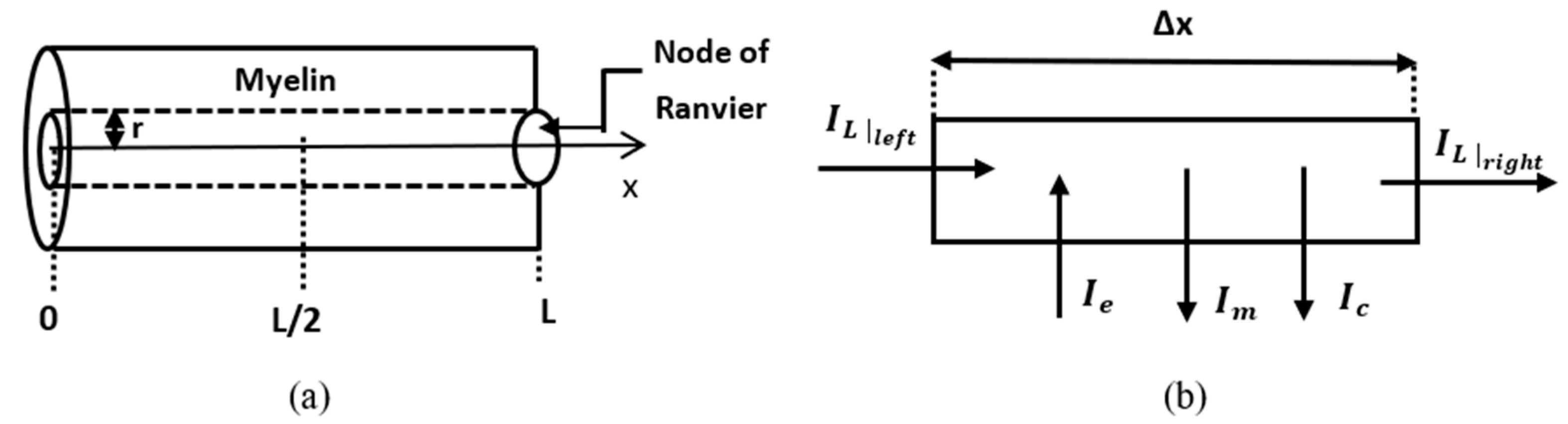
Definition 2.

The non-local voltage of order $\mathbf{\alpha }\left(t\right)=\left({\alpha }_1\left(t\right), {\alpha }_2\left(t\right), {\alpha }_3\left(t\right)\right), {\alpha }_i\left(t\right)>0, i=1,2,3$ between two points in ${\mathbf{R}}^3$ of position vectors $\mathbf{0}=\left(0, 0, 0\right)$ and $\mathbf{x}=\left(x_1, x_2, x_3\right) \in \left(\mathbf{0},\mathbf{R}\right), \mathbf{R}=\left(R_1, R_2, R_3\right)$is

$$\begin{array}{cc}V\left(\mathbf{x},t\right)& =-\frac{p}{L_1^{{\alpha }_1\left(t\right)-1}\mathsf{\Gamma }\left({\alpha }_1\left(t\right)\right)}\underset{0}{\overset{x_1}{{\displaystyle \int }}}{\left(x_1-y_1\right)}^{{\alpha }_1\left(t\right)-1}{E}_1\left(\mathbf{y},t\right)d{y}_1\\ & -\frac{p}{L_2^{{\alpha }_2\left(t\right)-1}\mathsf{\Gamma }\left({\alpha }_2\left(t\right)\right)}\underset{0}{\overset{x_2}{{\displaystyle \int }}}{\left(x_2-y_2\right)}^{{\alpha }_2\left(t\right)-1}{E}_2\left(\mathbf{y},t\right)d{y}_2\\ & -\frac{p}{L_3^{{\alpha }_3\left(t\right)-1}\mathsf{\Gamma }\left({\alpha }_3\left(t\right)\right)}\underset{0}{\overset{x_3}{{\displaystyle \int }}}{\left(x_3-y_3\right)}^{{\alpha }_3\left(t\right)-1}{E}_3\left(\mathbf{y},t\right)d{y}_3\\ & -\frac{q}{L_1^{{\alpha }_1\left(t\right)-1}\mathsf{\Gamma }\left({\alpha }_1\left(t\right)\right)}\underset{x_1}{\overset{R_1}{{\displaystyle \int }}}{\left(y_1-x_1\right)}^{{\alpha }_1\left(t\right)-1}{E}_1\left(\mathbf{y},t\right)d{y}_1\\ & -\frac{q}{L_2^{{\alpha }_2\left(t\right)-1}\mathsf{\Gamma }\left({\alpha }_2\left(t\right)\right)}\underset{x_2}{\overset{R_2}{{\displaystyle \int }}}{\left(y_2-x_2\right)}^{{\alpha }_2\left(t\right)-1}{E}_2\left(\mathbf{y},t\right)d{y}_2\\ & -\frac{q}{L_3^{{\alpha }_3\left(t\right)-1}\mathsf{\Gamma }\left({\alpha }_3\left(t\right)\right)}\underset{x_3}{\overset{R_3}{{\displaystyle \int }}}{\left(y_3-x_3\right)}^{{\alpha }_3\left(t\right)-1}{E}_3\left(\mathbf{y},t\right)d{y}_3\end{array}$$

(12)

where $\mathbf{E}\left(\mathbf{y},t\right)=\left(E_1\left(\mathbf{y},t\right), E_2\left(\mathbf{y},t\right), E_3\left(\mathbf{y},t\right)\right)$ is the electric field vector, $t\ge 0$ is a non-dimensional time, and $L_i, i=1, 2, 3$ are characteristic lengths. The positive constants $p$ and $q$ satisfy the constraint $p+q=1.$ For mathematical convenience, let $V\left(\mathbf{0}\right)=0$.

For now, the time-dependent, spatial, non-local effects are neglected. Because the axonal branches are long and narrow, the action potentials depend only on one spatial variable [33] and thus the problem is one-dimensional. Thus, the axon can be modeled as a circular cylinder of constant radius $r$ and one characteristic length $L,$ the length of the internodal region, and assume that

$${\alpha }_1\left(t\right)={\alpha }_2\left(t\right)={\alpha }_3\left(t\right)=\alpha =\mathrm{constant}, 0<\alpha \le 1.$$

(13)

In this case, the element of the path along the integration of $\overrightarrow{E}$ (a generalization of a measure proposed in [34]):

$$d{\mathbf{y}}_{\alpha \left(t\right)}=\left(\frac{1}{\mathsf{\Gamma }\left({\alpha }_1\left(t\right)\right)}{y}_1^{{\alpha }_1\left(t\right)-1}d{y}_1,\frac{1}{\mathsf{\Gamma }\left({\alpha }_2\left(t\right)\right)}{y}_2^{{\alpha }_2\left(t\right)-1}d{y}_2, \frac{1}{\mathsf{\Gamma }\left({\alpha }_3\left(t\right)\right)}{y}_3^{{\alpha }_3\left(t\right)-1}d{y}_3\right)$$

reduces to

$$d{\mathbf{y}}_{\alpha }=\frac{{\mathbf{y}}^{\alpha -1}}{\mathsf{\Gamma }\left(\alpha \right)}d\mathbf{y}=d\left[\frac{{\mathbf{y}}^{\alpha }}{\mathsf{\Gamma }\left(\alpha +1\right)}\right].$$

(14)

since $\alpha \mathsf{\Gamma }\left(\alpha \right)=\mathsf{\Gamma }\left(\alpha +1\right).$

The electric field is assumed to be uniform along the axon and the standard convention of current direction is valid: the membrane and synaptic current are positive when they are outward, and the electrode currents are positive when they are inward. Then, by using Expression (14), Formula (12) becomes

$$\begin{array}{cc}V\left(x,t\right)& =-\frac{Ep}{L^{\alpha -1}}{{\displaystyle \int }}_0^{x}d{\left(x-y\right)}_{\alpha }-\frac{Eq}{L^{\alpha -1}}{{\displaystyle \int }}_x^{R}d{\left(y-x\right)}_{\alpha }=-\frac{Ep}{L^{\alpha -1}}{{\displaystyle \int }}_0^{x}d\left[\frac{{\left(x-y\right)}^{\alpha }}{\mathsf{\Gamma }\left(\alpha +1\right)}\right]\\ & -\frac{Eq}{L^{\alpha -1}}{{\displaystyle \int }}_x^{R}d\left[\frac{{\left(y-x\right)}^{\alpha }}{\mathsf{\Gamma }\left(\alpha +1\right)}\right]=\frac{E}{L^{\alpha -1}}\frac{p{x}^{\alpha }-q{\left(R-x\right)}^{\alpha }}{\mathsf{\Gamma }\left(\alpha +1\right)}.\end{array}$$

(15)

Comparing Formulas (15) and (6) gives

$$V\left(x,t\right)=p{I}_{0+}^{\alpha }\left(\frac{E}{L^{\alpha -1}}\right)-q{I}_{R-}^{\alpha }\left(\frac{E}{L^{\alpha -1}}\right).$$

Consider an equally spaced discretization of $\left[0, R\right]$ with step size $\mathsf{\Delta }x$ and the number of nodes chosen such that, when $\alpha =1$, the following formula reduces to the classic forward approximation of the first-order derivative. Then Formula (15) yields

$$\mathsf{\Delta }V\left(x,t\right)=V\left(x+\mathsf{\Delta }x,t\right)-V\left(x,t\right)=\frac{E}{L^{\alpha -1}\mathsf{\Gamma }\left(\alpha +1\right)}\left({\left(x+\mathsf{\Delta }x\right)}^{\alpha }-x^{\alpha }\right).$$

(16)

On the other hand, using Formula (11) and the fact that $p+q=1$ give

$$\begin{array}{lll}\mathsf{\Delta }V\left(x,t\right)& =& \left(p+q\right)V\left(x+\mathsf{\Delta }x,t\right)-\left(p+q\right)V\left(x,t\right)\\ & \approx & \frac{p{D}_{0+}^{\alpha }V\left(x,t\right)+q{\left(-1\right)}^{\alpha }{D}_{R-}^{\alpha }V\left(x,t\right)}{\mathsf{\Gamma }\left(\alpha +1\right)}\left({\left(x+\mathsf{\Delta }x\right)}^{\alpha }-x^{\alpha }\right)\end{array}$$

(17)

where the Caputo fractional derivatives are taken with respect to the spatial variable $x$.

Thus, as $\mathsf{\Delta }x\to 0$, Formulas (16) and (17) yield

$$p{D}_{0+}^{\alpha }V\left(x,t\right)+q{\left(-1\right)}^{\alpha }{D}_{R-}^{\alpha }V\left(x,t\right)=\frac{E}{L^{\alpha -1}} .$$

(18)

The uniformity of the current density in every cross-sectional area of the cylindrical neuron gives [33]

$$E=\frac{r_{L}I}{\pi r^2}$$

(19)

where $r_L$ is the intracellular resistance and $I$ is the electric current. Combining Formulas (18) and (19) gives the expression of the longitudinal current:

$$I_L=-\frac{\pi r^2{L}^{\alpha -1}}{r_L}\left[p D_{0+}^{\alpha }V\left(x,t\right)+q{\left(-1\right)}^{\alpha } D_{R-}^{\alpha }V\left(x,t\right)\right]$$

(20)

where the negative sign comes from the current sign convention. Replacing Formula (19) into Formula (16) also yields Ohm’s law:

$$\mathsf{\Delta }V\left(x,t\right)=R_{\alpha }I$$

for the generalized electric resistance:

$$R_{\alpha }=\frac{r_L}{\pi r^2{L}^{\alpha -1}\mathsf{\Gamma }\left(\alpha +1\right)}\left({\left(x+\mathsf{\Delta }x\right)}^{\alpha }-x^{\alpha }\right).$$

(21)

As in [17,33,35], the following currents are introduced:

$$\begin{gathered} I_m=2\pi r \mathsf{\Delta }x i_m \\ {I}_e=2\pi r \mathsf{\Delta }x i_e \\ {I}_c=2\pi r \mathsf{\Delta }x c_m^{*}{\partial }_{0+}^{\beta }V, 0<\beta \le 1 \end{gathered}$$

(22)

where $I_m$ and $I_e$ are the membrane and external currents, respectively, and $i_m$ and $i_e$ are their corresponding currents per unit area. The capacitor current is $I_c$ and

$$c_m=\frac{c_m^{*}}{T^{\beta -1}}$$

(23)

where $c_m$ is the specific membrane capacitance, and $T$ is a characteristic time. The use of a temporal Caputo fractional derivative in the expression of $I_c$ was justified in [17] as giving a more accurate characterization of experimentally observed propagation of action potentials.

The replacement of Formulas (20) and (22) in Kirchhoff’s law in the element is shown in Figure 2b:

$$I_c+I_m-I_{L|left}+I_{L|right}-I_e=0$$

(24)

gives

$$\begin{gathered} c_m^{*}{\partial }_{0+}^{\beta }V= i_e-i_m \\ +\frac{r}{2{\tilde{r}}_L}\frac{{\left[p D_{0+}^{\alpha }V\left(x,t\right)+q{\left(-1\right)}^{\alpha } D_{R-}^{\alpha }V\left(x,t\right)\right]}_{|right}-{\left[p D_{0+}^{\alpha }V\left(x,t\right)+q{\left(-1\right)}^{\alpha } D_{R-}^{\alpha }V\left(x,t\right)\right]}_{|left}}{\mathsf{\Delta }x} \end{gathered}$$

(25)

where

$${\tilde{r}}_L=\frac{r_L}{L^{\alpha -1}} .$$

(26)

As $\mathsf{\Delta }x\to 0$:

$$\begin{gathered} \frac{{\left[p D_{0+}^{\alpha }V\left(x,t\right)+q{\left(-1\right)}^{\alpha } D_{R-}^{\alpha }V\left(x,t\right)\right]}_{|right}-{\left[p D_{0+}^{\alpha }V\left(x,t\right)+q{\left(-1\right)}^{\alpha } D_{R-}^{\alpha }V\left(x,t\right)\right]}_{|left}}{\mathsf{\Delta }x} \\ \approx \frac{\partial }{\partial x}\left[p D_{0+}^{\alpha }V\left(x,t\right)+q{\left(-1\right)}^{\alpha } D_{R-}^{\alpha }V\left(x,t\right)\right] \end{gathered}$$

which replaced in Equation (25) and letting $\mathsf{\Delta }x\to 0$ give the expression of the spatio-temporal fractional cable equation:

$$c_m^{*}{\partial }_{0+}^{\beta }V=\frac{r}{2{\tilde{r}}_L}\left[p\frac{\partial }{\partial x}\left(D_{0+}^{\alpha }V\right)+q{\left(-1\right)}^{\alpha }\frac{\partial }{\partial x}\left(D_{R-}^{\alpha }V\right)\right]+i_e-i_m.$$

(27)

If $V\left(0,t\right)=V\left(R,t\right)=0$, then Equation (27) can be written in the equivalent form:

$$c_m^{*}{\partial }_{0+}^{\beta }V=\frac{r}{2{\tilde{r}}_L}\left[p{D}_{0+}^{\alpha +1}V+q{\left(-1\right)}^{\alpha +1}{D}_{R-}^{\alpha +1}V\right]+i_e-i_m.$$

(28)

For $p=1,q=0$ (or $p=0,q=1$) and $\alpha =\beta =1$, Equation (27) reduces to the classic cable equation [33]:

$$c_m\frac{\partial V}{\partial t}=\frac{r}{2r_L}\frac{{\partial }^{2}V}{\partial x^2}+i_e-i_m.$$

(29)

A numerical discretization of the second-order spatial derivative in Equation (29) shows that in myelinated neurons the voltage at node $n$ depends only on the voltages at the adjacent nodes of Ranvier, $n-1$ and $n+1$. However, a numerical discretization of the spatial Caputo fractional derivatives in Equation (27) based on the Gr$\ddot{\mathrm{u}}$nwald–Letnikov formula (see later) shows that the voltage at node $n$ depends on the voltages at all the previous nodes $0, 1, \dots , n-1$, and all the following nodes $n+1, n+2, \dots n+N$, where $N$ is the total number of nodes of an axon. The Gr$\ddot{\mathrm{u}}$nwald–Letnikov formula can also be used to approximate numerically the temporal Caputo fractional derivative in Equation (27). (Although, in this paper, a different numerical scheme is applied to discretize the temporal Caputo fractional derivative (see later), it is somehow easier to mention the Gr$\ddot{\mathrm{u}}$nwald–Letnikov formula here to highlight temporal non-locality.) Thus, Equation (27) models the long-term memory and long-range interactions of the voltage in myelinated neurons.

Near the resting potential $V_{rest}$ the membrane current per unit area can be approximated as [33]

$$i_m=\frac{V-V_{rest}}{r_m}:=\frac{v}{r_m}$$

(30)

where $v=V-V_{rest}$ is the voltage relative to the resting potential, and $r_m$ is the specific membrane resistance. Since $V_{rest}$ is constant, it follows from Formula (8) that

$$D_{0+}^{\alpha }V=D_{0+}^{\alpha }v,\hspace{1em}\hspace{1em}{D}_{R-}^{\alpha }V=D_{R-}^{\alpha }v,\hspace{1em}\hspace{1em}{\partial }_{0+}^{\beta }V={\partial }_{0+}^{\beta }v.$$

Thus, Equation (27) becomes

$${\tau }_m{\partial }_{0+}^{\beta }v={\lambda }^{\alpha +1}\left[p\frac{\partial }{\partial x}\left(D_{0+}^{\alpha }v\right)+q{\left(-1\right)}^{\alpha }\frac{\partial }{\partial x}\left(D_{R-}^{\alpha }v\right)\right]+r_m{i}_e-v$$

(31)

where

$${\tau }_m=r_m{c}_m^{*}=r_m{c}_m{T}^{\beta -1}, {\lambda }^{\alpha +1}=\frac{r{r}_m}{2 r_L}{L}^{\alpha -1}.$$

(32)

The generalized electrotonic length $\lambda$ has the same expression as in [16] and captures the effect of spatial non-locality via the parameter $\alpha \in \left(0,1\right)$ on the relationship among the geometric parameters $r, L$ and the resistances $r_m, r_L$ of a neuron. Parameter $\beta \in \left(0,1\right)$ controls the time scale and accounts for long-term memory effects. Since Equation (27) remains valid for a time-varying $\alpha \left(t\right)$, the variations of $\alpha \left(t\right)$ and $\beta$, and the interplay between them, may reveal how aging and myelin assembly and remodeling affect the timing, speed, and shape of the action potentials.

3.1. Dynamic Problem

In this sub-section, a numerical solution to Equation (31) coupled with the fractional Hodgkin–Huxley equations is presented. The problem is stated and solved numerically in a leaky internodal region of length $L$ with one isopotential node at $x=L$ (Figure 2a). The assumption that the length of the node of Ranvier can be neglected in the model is supported by the fact that in most neurons the length of the internodal region is of the order $1000÷2000 \mathsf{\mu }\mathrm{m}$, which is much bigger than the usual nodal length of about $3 \mathsf{\mu }\mathrm{m}$ [36]. It is also assumed that the potential $v\left(x,t\right)$ is zero at the middle of the internodal region and symmetric about the vertical line $x=L/2$. Thus, the spatial domain is $\left[L/2,L\right].$ The membrane potential of the internodal region is the solution to the following initial boundary value problem:

$$\begin{gathered} {\tau }_m{\partial }_{0+}^{\beta }v={\lambda }^{\alpha +1}\left[p\frac{\partial }{\partial x}\left(D_{0.5L+}^{\alpha }v\right)+q{\left(-1\right)}^{\alpha }\frac{\partial }{\partial x}\left(D_{L-}^{\alpha }v\right)\right]-v, \\ x\in \left(\frac{L}{2},L\right) \end{gathered}$$

(33)

$$v\left(x,0\right)=0, v\left(L/2,t\right)=0, v\left(L,t\right)=f\left(t\right)$$

(34)

where $f\left(t\right)=V\left(t\right)-V_{rest}$ and $V\left(t\right)$, the membrane potential of the node, is the solution of the following fractional Hodgkin–Huxley model, adapted from [37]:

$$c_m^{*}{\partial }_{0+}^{\beta }V=I-\left(G_{Na}{m}^{3}h+G_{NaL}\right)\left(V-E_{Na}\right)-\left(G_K{n}^4+G_{KL}\right)\left(V-E_K\right)-G_{ClL}\left(V-E_{Cl}\right),$$

(35)

$$T^{\beta -1}{\partial }_{0+}^{\beta }m={\alpha }_m\left(1-m\right)-{\beta }_{m}m,$$

(36)

$$T^{\beta -1}{\partial }_{0+}^{\beta }n={\alpha }_n\left(1-n\right)-{\beta }_{n}n,$$

(37)

$$T^{\beta -1}{\partial }_{0+}^{\beta }h={\alpha }_h\left(1-h\right)-{\beta }_{h}h$$

(38)

with initial conditions

$$\begin{array}{c}V\left(0\right)=V_{rest} ,\\ m\left(0\right)=\frac{{\alpha }_m\left(V\left(0\right)\right)}{{\alpha }_m\left(V\left(0\right)\right)+{\beta }_m\left(V\left(0\right)\right)},\\ n\left(0\right)=\frac{{\alpha }_n\left(V\left(0\right)\right)}{{\alpha }_n\left(V\left(0\right)\right)+{\beta }_n\left(V\left(0\right)\right)},\\ h\left(0\right)=\frac{{\alpha }_h\left(V\left(0\right)\right)}{{\alpha }_h\left(V\left(0\right)\right)+{\beta }_h\left(V\left(0\right)\right)},\end{array}$$

(39)

where

$$\begin{array}{c}{\alpha }_m=\frac{0.32\left(V+54\right)}{1-\exp \left(-0.25\left(V+54\right)\right)}, {\beta }_m=\frac{0.28\left(V+27\right)}{\exp \left(0.2\left(V+27\right)\right)-1},\\ {\alpha }_n=\frac{0.032\left(V+52\right)}{1-\exp \left(-0.2\left(V+52\right)\right)}, {\beta }_n=0.5\exp \left(-\frac{V+57}{40}\right),\\ {\alpha }_h=0.128\exp \left(-\frac{V+50}{18}\right), {\beta }_h=\frac{4}{1+\exp \left(-0.2\left(V+27\right)\right)}.\end{array}$$

(40)

In Equations (35)–(38), $I$ is an externally applied current per unit area; $E_{Na}, E_K,$ and $E_{Cl}$ are the reverse potentials; and $G_{Na}, G_K, G_{NaL},G_{KL},$ and $G_{ClL}$ are, respectively, the voltage-gated maximal conductances of $N{a}^{+}$ and $K^{+}$, and the leak conductances of $N{a}^{+}, K^{+},$ and $C{l}^{-}$. The gating variables $m, n,$ and $h$ are the activations of the $N{a}^{+}$ and $K^{+}$ channels and the inactivation of the $N{a}^{+}$ channel, respectively. Parameters ${\alpha }_m, {\alpha }_n, {\alpha }_h, {\beta }_m, {\beta }_n,$ and ${\beta }_h$ were found by fitting the classic Hodgkin–Huxley model ($\beta =1$ in Equations (35)–(38)) to experimental data (see, for instance, Section 2.2 of [38] and references within) and thus they should not be confused with the newly introduced non-local parameters $\alpha$ and $\beta$.

3.2. Numerical Discretization

A numerical discretization of the right-hand side of Equation (33) is given first.

Let $L/2=x_0<x_1<\cdots <x_{N-1}<x_N=L$ be an equally spaced discretization of the interval $\left[L/2,L\right]$ of constant step size $\mathsf{\Delta }x$. The spatial fractional derivatives are approximated using the right- and left-shifted Gr$\ddot{\mathrm{u}}$nwald–Letnikov formulas given in [18,39] and the boundary conditions in (34) (the link between the Caputo fractional derivatives and the $\mathrm{Gr}\ddot{\mathrm{u}}\mathrm{nwald}$–Letnikov formulas is established through an integration by parts):

$$\begin{gathered} \frac{\partial }{\partial x}\left(D_{0.5L+}^{\alpha }v\left(x_j,t\right)\right)=\frac{1}{\Delta x^{\alpha +1}}{\displaystyle \sum }_{i=0}^{j+1}{g}_i^{\alpha +1}v\left(x_{j-i+1},t\right), 0<j<N \\ \frac{\partial }{\partial x}\left(D_{L-}^{\alpha }v\left(x_j,t\right)\right)=\frac{-1}{\Delta x^{\alpha +1}}{\displaystyle \sum }_{i=0}^{N-j+1}{g}_i^{\alpha +1}v\left(x_{j+i-1},t\right)+\frac{f\left(t\right)}{\mathsf{\Gamma }\left(-\alpha \right){\left(L-x_j\right)}^{\alpha +1}}, 0<j<N \end{gathered}$$

(41)

where

$$g_i^{\alpha +1}=\frac{{\left(-1\right)}^i\mathsf{\Gamma }\left(\alpha +2\right)}{\mathsf{\Gamma }\left(i+1\right)\mathsf{\Gamma }\left(\alpha -i+2\right)} , g_0^{\alpha +1}=1.$$

(42)

Formula (41) can be re-written by changing the indexes of the terms in the sums:

$$\frac{\partial }{\partial x}\left(D_{0.5L+}^{\alpha }v\left(x_j,t\right)\right)=\frac{1}{\Delta x^{\alpha +1}}{\displaystyle \sum }_{k=0}^{j+1}{g}_{j+1-k}^{\alpha +1}v\left(x_k,t\right), 0<j<N$$

(43)

$$\frac{\partial }{\partial x}\left(D_{L-}^{\alpha }v\left(x_j,t\right)\right)=\frac{-1}{\Delta x^{\alpha +1}}{\displaystyle \sum }_{k=j-1}^N{g}_{k+1-j}^{\alpha +1}v\left(x_k,t\right)+\frac{f\left(t\right)}{\mathsf{\Gamma }\left(-\alpha \right){\left(L-x_j\right)}^{\alpha +1}}, 0<j<N$$

(44)

As in [18], Formula (43) introduces the following matrix $\widehat{L}$ of dimension $\left(N-1\right)\times \left(N-1\right)$:

$${\widehat{L}}_{jk}=\{\begin{array}{lll}{g}_{j+1-k}^{\alpha +1},& 1\le j\le N-1,& 1\le k\le j\\ 1,& 1\le j<N-1,& k=j+1\\ & 0,& \mathrm{otherwise}\end{array}$$

Similarly, a matrix $\check{L}$ of dimension $\left(N-1\right)\times \left(N-1\right)$ corresponding to Formula (44) can be introduced. However, using Formula (42), it is easy to show that $\check{L}={\widehat{L}}^T$. The terms involving the boundary conditions in Formulas (43) and (44) are not included in the expressions of matrices $\widehat{L}$ and $\check{L}.$ The boundary terms are collected from the sums in Formulas (43) and (44) and stored in the following vectors:

$${\widehat{b}}_j=\{\begin{array}{ll}0,& 1\le j\le N-2\\ f\left(t\right),& j=N-1\end{array}, {\check{b}}_j=f\left(t\right)g_{N+1-j}^{\alpha +1} , 1\le j\le N-1$$

(45)

where the boundary conditions (34) have been used.

Replacing Formulas (43)–(45) in Equation (33) and grouping the like terms give

$${\partial }_{0+}^{\beta }v\left(x_j,t\right)={\displaystyle \sum }_{k=1}^{N-1}{B}_{jk}v\left(x_k,t\right)+b_j+d_j, 1\le j\le N-1$$

(46)

where

$$B_{jk}=\frac{{\lambda }^{\alpha +1}}{{\tau }_m\mathsf{\Delta }{x}^{\alpha +1}}\left(p{\widehat{L}}_{jk}+q{\left(-1\right)}^{\alpha +1}{\widehat{L}}_{kj}\right)-\frac{1}{{\tau }_m}{\delta }_{jk}, 1\le j,k\le N-1$$

with ${\delta }_{jk}$ the Kronecker delta function,

$$b_j=\frac{{\lambda }^{\alpha +1} }{{\tau }_m\mathsf{\Delta }{x}^{\alpha +1}}\left[p{\widehat{b}}_j+q{\left(-1\right)}^{\alpha +1}{\check{b}}_j\right], 1\le j\le N-1$$

and the last term of Formula (44) is stored in the following vector:

$$d_j=q{\left(-1\right)}^{\alpha }\frac{{\lambda }^{\alpha +1} f\left(t\right)}{{\tau }_m\mathsf{\Delta }{x}^{\alpha +1}}\frac{1}{\mathsf{\Gamma }\left(-\alpha \right){\left(N-j\right)}^{\alpha +1}} , 1\le j\le N-1.$$

The real part of ${\left(-1\right)}^{\alpha }$ is used in the numerical simulations.

Equations (46) and (35)–(38) form a system of coupled, non-linear, fractional ordinary differential equations that needs to be solved numerically using the initial conditions (34) and (39). Let

$$\begin{gathered} u_j\left(t\right)=v\left(x_j,t\right) , 1\le j\le N-1, \\ {u}_N\left(t\right)=V\left(t\right), u_{N+1}\left(t\right)=m\left(t\right), u_{N+2}\left(t\right)=n\left(t\right), u_{N+3}\left(t\right)=h\left(t\right). \end{gathered}$$

Then, Equations (46) and (35)–(38) can be written in compact form:

$${\partial }_{0+}^{\beta }{u}_j\left(t\right)=F_j\left(t,u_1\left(t\right),\dots ,u_{N+3}\left(t\right)\right), 1\le j\le N+3$$

(47)

where $F_j\left(t\right), 1\le j\le N+3,$ are the corresponding right-hand sides of Equations (46) and (35)–(38). The initial conditions (34) and (39) are denoted by $u_{j,0}, 1\le j\le N+3.$ A numerical discretization of system (47) is presented next.

The fractional Hodgkin–Huxley equations in [17,35] were solved using either a non-standard finite difference scheme [35] that combines the Gr$\ddot{\mathrm{u}}$nwald–Letnikov formula and a denominator function dependent on the step size satisfying certain conditions, or a semi-analytic approach [17] that involves the predator-corrector method given in [40]. The numerical scheme used in this paper is a variant of the one in [40]. More precisely, system (47) is solved numerically using MATLAB’s function fde12 [19], which is an implementation of (1) a modified predictor–corrector method, which combines generalizations of the Adam–Bashforth (predictor) and Adam–Moulton (corrector) methods [41]; and (2) a fast Fourier transform (FFT) algorithm that reduces the computational cost [42]. For the sake of completeness, the main steps of the modified predictor-corrector method in [40,41] are presented further.

Applying the left-sided Riemann–Liouville fractional integral of order $\beta \in \left(0,1\right)$ to system (47) and using Formulas (9) and (6) give

$$u_j\left(t\right)=u_{j,0}+\frac{1}{\mathsf{\Gamma }\left(\beta \right)}{{\displaystyle \int }}_0^t{\left(t-s\right)}^{\beta -1}{F}_j\left(s,u_1\left(s\right),\dots ,u_{N+3}\left(s\right)\right)ds, 1\le j\le N+3$$

(48)

Let $0=t_0<t_1<\dots <t_M$ be an equally spaced discretization of a time interval $\left[0,t\right]$ with constant step size $\mathsf{\Delta }t$, denoted by $u_j\left(t_n\right)=u_j^n.$

The generalization of the Adams–Bashforth method involves the use of the product rectangle rule to approximate:

$$\begin{gathered} {{\displaystyle \int }}_0^{t_{n+1}}{\left(t_{n+1}-s\right)}^{\beta -1}{F}_j\left(s,u_1\left(s\right),\dots ,u_{N+3}\left(s\right)\right)ds\approx {\displaystyle \sum }_{k=0}^n{\widehat{a}}_{k,n+1}{F}_j\left(t_k,u_1^k,\dots ,u_{N+3}^k\right), \\ 1\le j\le N+3 \end{gathered}$$

(49)

where

$${\widehat{a}}_{k,n+1}={{\displaystyle \int }}_{t_k}^{t_{k+1}}{\left(t_{n+1}-s\right)}^{\beta -1}ds=\frac{\Delta t^{\beta }}{\beta }\left[{\left(n+1-k\right)}^{\beta }-{\left(n-k\right)}^{\beta }\right].$$

By replacing Formula (49) in Expression (48), the predator formula is obtained:

$$u_j^{n+1,P}\left(t\right)=u_{j,0}+\frac{1}{\mathsf{\Gamma }\left(\beta \right)}{\displaystyle \sum }_{k=0}^n{\widehat{a}}_{k,n+1}{F}_j\left(t_k,u_1^k,\dots ,u_{N+3}^k\right), 1\le j\le N+3.$$

(50)

The generalization of the Adams–Moulton method involves the use of the product trapezoidal quadrature formula to approximate:

$$\begin{gathered} {{\displaystyle \int }}_0^{t_{n+1}}{\left(t_{n+1}-s\right)}^{\beta -1}{F}_j\left(s,u_1\left(s\right),\dots ,u_{N+3}\left(s\right)\right)ds\approx {\displaystyle \sum }_{k=0}^{n+1}{\check{a}}_{k,n+1}{F}_j\left(t_k,u_1^k,\dots ,u_{N+3}^k\right), \\ 1\le j\le N+3 \end{gathered}$$

(51)

where a piecewise linear interpolant of $F_j$ is used on the left-hand side of Formula (51).

Thus,

$$\begin{array}{ll}{\check{a}}_{k,n+1}& ={{\displaystyle \int }}_0^{t_{n+1}}{\left(t_{n+1}-s\right)}^{\beta -1}{\phi }_{k,n+1}\left(s\right)ds\\ & =\frac{\Delta t^{\beta }}{\beta \left(\beta +1\right)}\{\begin{array}{ll}\left(n^{\beta +1}-\left(n-\beta \right){\left(n+1\right)}^{\beta }\right),& k=0\\ \left({\left(n-k+2\right)}^{\beta +1}-2{\left(n-k+1\right)}^{\beta +1}+{\left(n-k\right)}^{\beta +1}\right),& 1\le k\le n\\ 1,& k=n+1\end{array}\end{array}$$

where ${\phi }_{k,n+1}$ are the piecewise linear (hat) basis functions associated with nodes $t_k, 0\le k\le n+1.$

By now replacing Formula (51) in Expression (48), the corrector formula is obtained:

$$u_j^{n+1}\left(t\right)=u_{j,0}+\frac{1}{\mathsf{\Gamma }\left(\beta \right)}{\displaystyle \sum }_{k=0}^n{\check{a}}_{k,n+1}{F}_j\left(t_k,u_1^k,\dots ,u_{N+3}^k\right)+\frac{1}{\mathsf{\Gamma }\left(\beta \right)}{\check{a}}_{n+1,n+1}{F}_j\left(t_{n+1},u_1^{n+1,P},\dots ,u_{N+3}^{n+1,P}\right), 1\le j\le N+3.$$

(52)

Lastly, the sums in the predictor and corrector Formulas (50) and (52) can be written as discrete convolutions, which are efficiently calculated using the FFT algorithm given in [42].

4. Results

The parameters used in the numerical simulations are given in

Table 1. List of parameters with corresponding values and physical units.

Parameters	Values and Units	Reference
$V_{rest}$	−65 $\mathrm{mV}$	[37]
$E_{Na}$	60 $\mathrm{mV}$	[37]
$E_K$	−88 $\mathrm{mV}$	[37]
$E_{Cl}$	−61 $\mathrm{mV}$	[37]
$G_{Na}$	0.3 $\mathrm{mS}/{\mathrm{mm}}^2$	[37]
$G_K$	0.25 $\mathrm{mS}/{\mathrm{mm}}^2$	[37]
$G_{NaL}$	0.000247 $\mathrm{mS}/{\mathrm{mm}}^2$	[37]
$G_{KL}$	0.0005 $\mathrm{mS}/{\mathrm{mm}}^2$	[37]
$G_{ClL}$	0.001 $\mathrm{mS}/{\mathrm{mm}}^2$	[37]
$c_m$	0.01 $\mathsf{\mu }\mathrm{F}/{\mathrm{mm}}^2$	[37]
$I$	0.1 $\mathsf{\mu }\mathrm{A}/{\mathrm{mm}}^2$
$r$	0.002 $\mathrm{mm}$	[33]
$r_m$	${10}^3 \mathrm{k}\mathsf{\Omega }·{\mathrm{mm}}^2$	[33]
$r_L$	1 $\mathrm{k}\mathsf{\Omega }·\mathrm{mm}$	[33]
$L$	1 $\mathrm{mm}$	[33]
$\alpha$	0.65 (0.25, 0.5, 0.85, 1)
$\beta$	0.66 (0.7, 0.8, 0.95, 1)

. The simulations use an internodal length of $L=1000 \mathsf{\mu }\mathrm{m}$, which gives the maximum propagation speed of an action potential [43]. This value of $L$ is within the range of values for the internodal length found in the literature ([44] gives $L=200 ÷2000 \mathsf{\mu }\mathrm{m}$ where the lower (higher) value corresponds to the initial myelination (full maturity) stage [45]). In the simulations, the time step size is $\Delta t=0.0001$ and the space step size $\Delta x=0.01$. 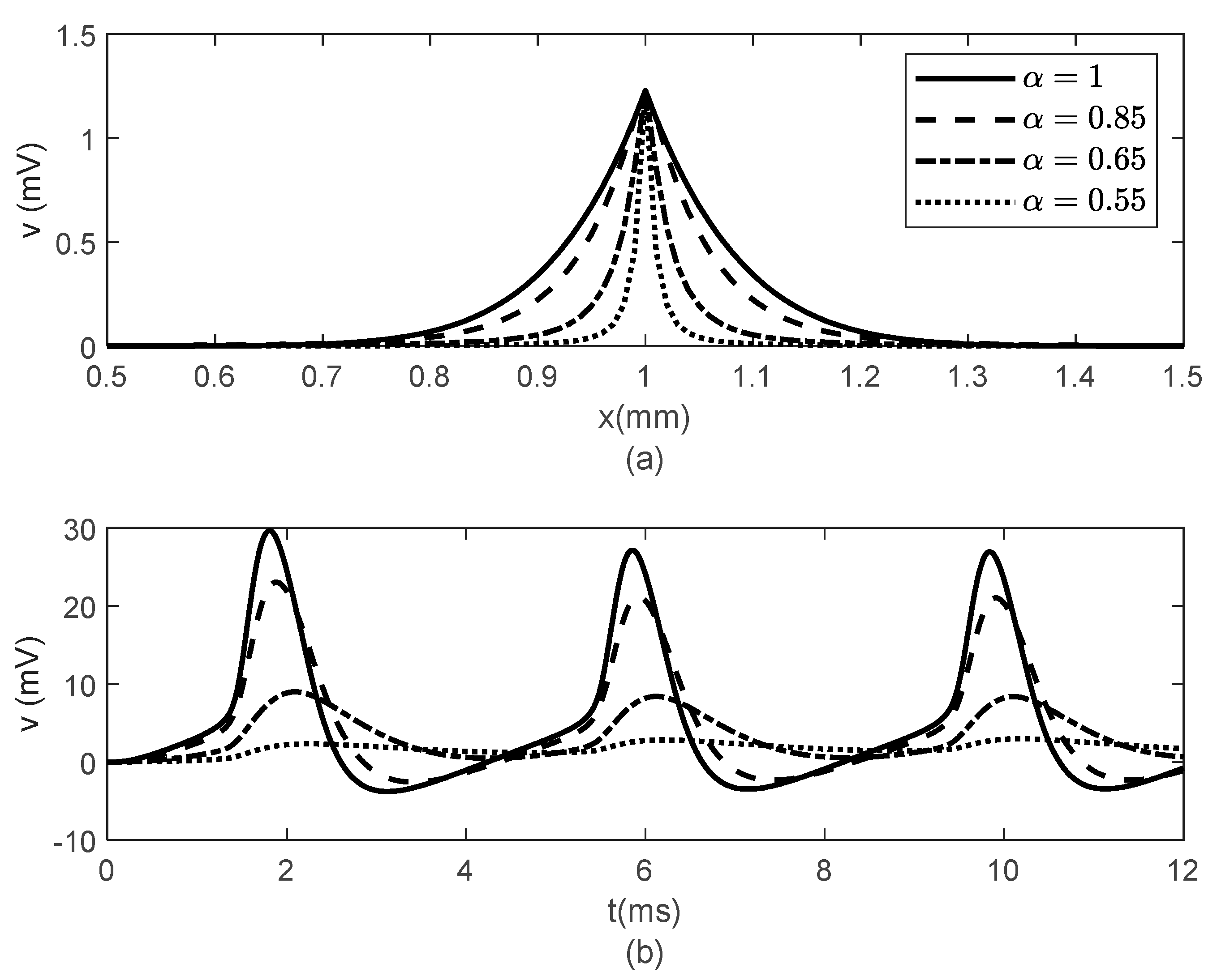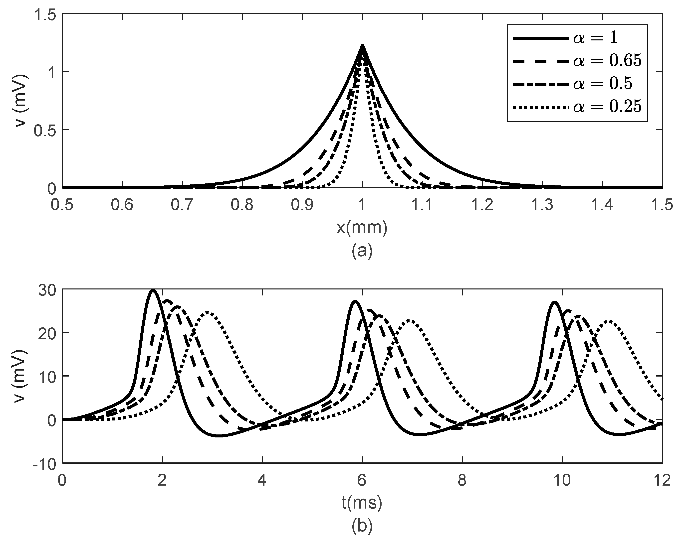For simplicity, $T=1.$ The plots showing the spatial variations of $v\left(x,t\right)$ (Figure 3a, Figure 4a, Figure 6a and Figure 8a) represent the solutions $v$ of problems (33)–(34) on the interval $\left[L/2,L\right]$ and their mirror images about the vertical line at the node of Ranvier. This approach offers a better visualization of the action potentials at the node of Ranvier for a fixed time.

Figure 3 and Figure 4 show spatial and temporal variations of $v\left(x,t\right)$ for $\beta =1$ and various values of $\alpha$ when $p=1, q=0$ (Figure 3) and $p=0, q=1$ (Figure 4). As expected, when $\alpha =1$, there is no difference between the two cases since the classic solution of the cable equation is recovered. At fixed time $t=0.1 \mathrm{ms}$, the shape of the action potentials at the node of Ranvier becomes narrower as $\alpha$ decreases, with the narrower shapes obtained for the case $p=0, q=1.$ (Figure 3a and Figure 4a). These spatially narrower action potentials at the nodes look like the ones in ([20], Figure 7D). In the case $p=0, q=1$, the numerical solution becomes unstable for $\alpha <0.55$. However, a solution in this scenario might not be physiologically meaningful since a too narrow action potential will lack the gradual spread of $v$ within the internodal region seen in optical recordings of membrane potentials [20]. At fixed location $x=700 \mathsf{\mu }\mathrm{m}$, the amplitude of $v$ decreases and shifts to the right as $\alpha$ decreases (Figure 3b and Figure 4b). The amplitude of $v$ decreases faster with decreasing $\alpha$ in the case $p=0, q=1$ (Figure 4b) than in the case $p=1, q=0$ (Figure 3b). This effect of the bidirectional propagation on the temporal variations of the membrane potential within the internodal region has not been observed experimentally. 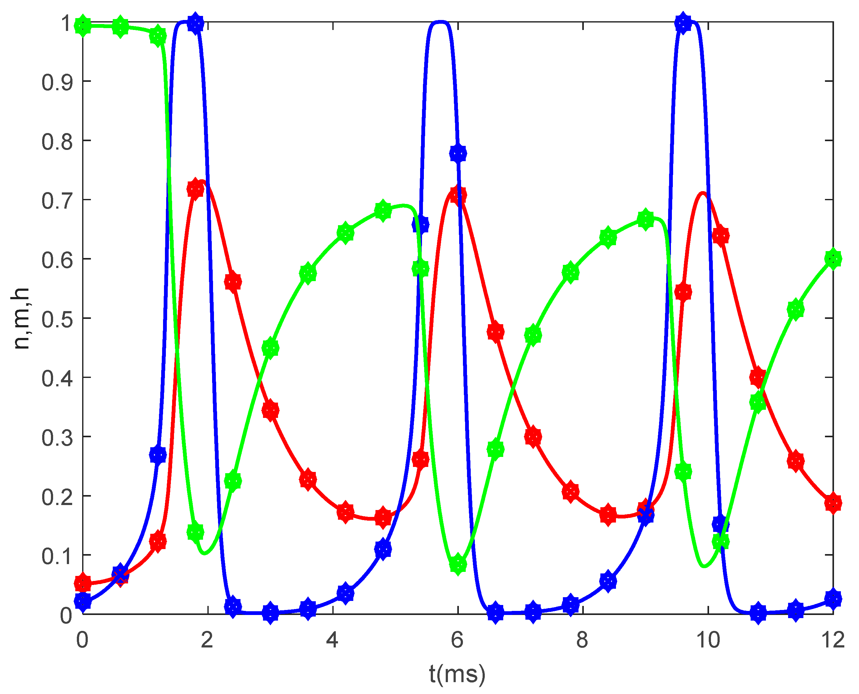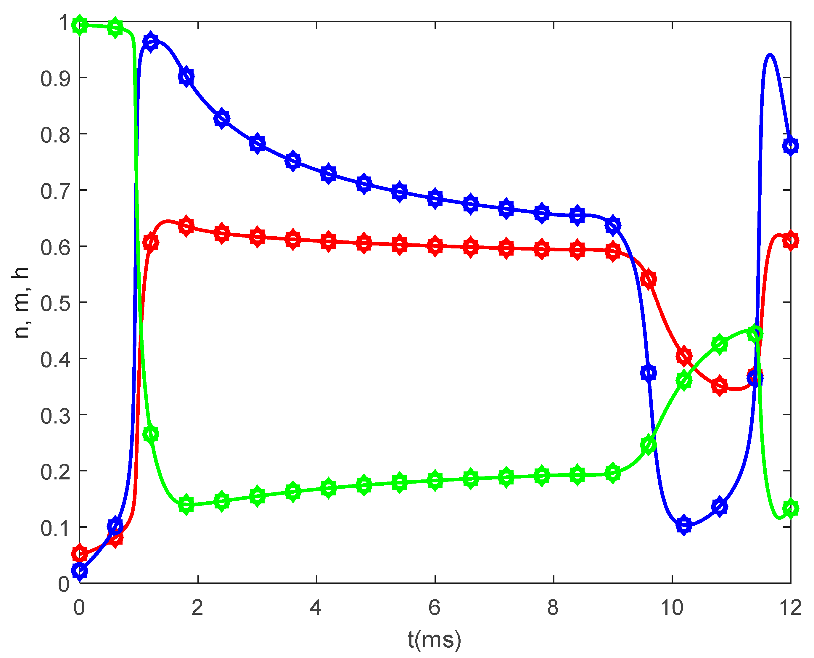Figure 5 shows the time variations of the gating variables $n\left(t\right), m\left(t\right),$ and $h\left(t\right)$ for $\beta =1$ and various values of $\alpha$ when $p=1, q=0$. Since the gating variables are independent of the spatial variable $x$, the values of $\alpha , p,$ and $q$ do not influence the variations of $n\left(t\right), m\left(t\right),$ and $h\left(t\right)$. Thus, the plots in Figure 5 are the solutions to the classic Hodgkin–Huxley equations.

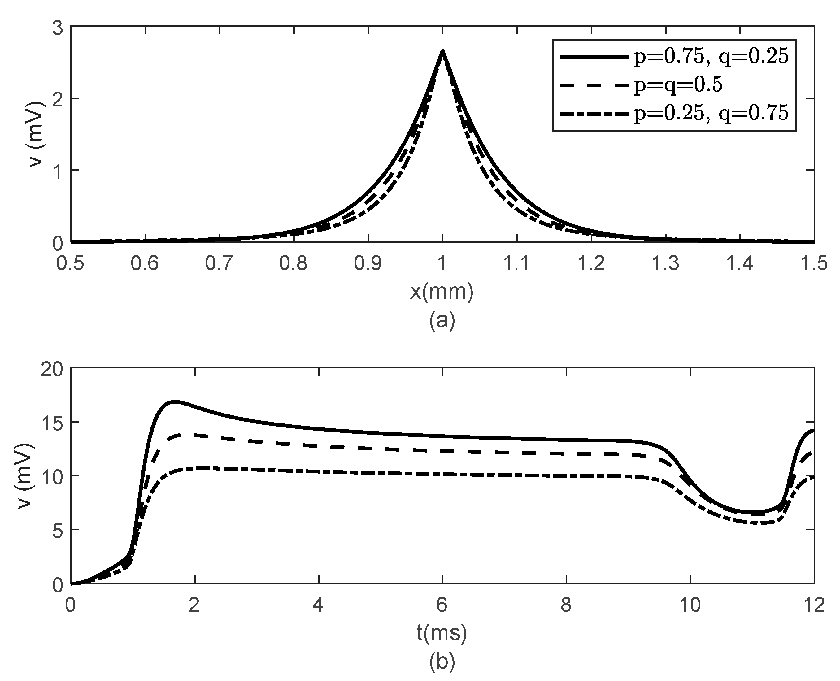
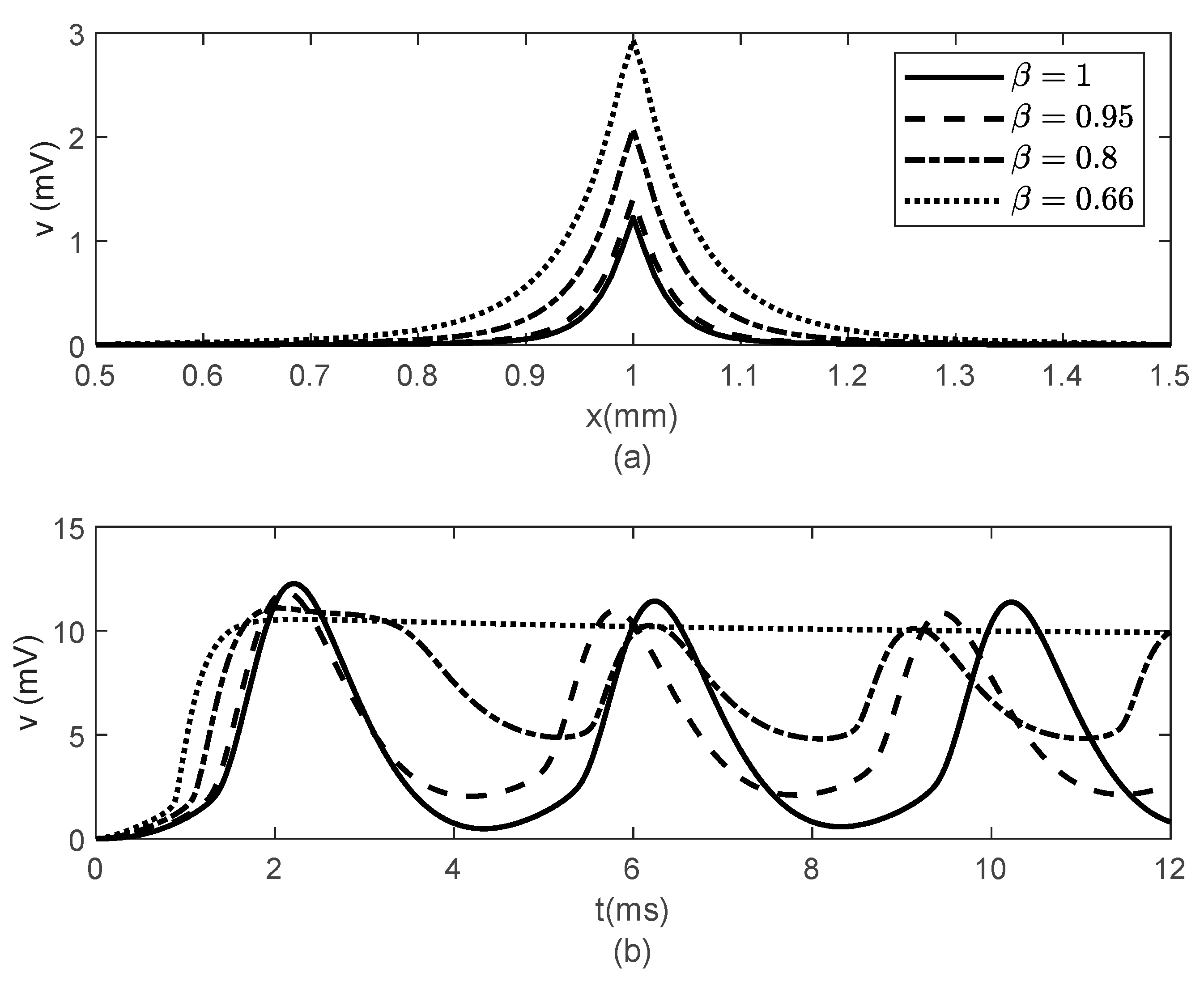
Figure 6 and Figure 7 show the results obtained for $\alpha =0.65$, $\beta =0.7$ and various values of $p, q$. While the width of the action potentials at the node of Ranvier and at the fixed time $t=0.1 \mathrm{ms}$ barely changes with decreasing $p$(increasing $q$) (Figure 6a), the amplitude of the potential $v$ at fixed location $x=700 \mathsf{\mu }\mathrm{m}$ decreases as $p$ decreases ($q$ increases) (Figure 6b). The long-term memory represented by $\beta =0.7<1$ causes delays in the opening and closing of the ion channels, which can be seen in the time variations of the gating variables $n\left(t\right), m\left(t\right),$ and $h\left(t\right)$ (Figure 7), which further produce the delay in the membrane potential seen in Figure 6b. Again, the values of $\alpha , p$ and $q$ do not influence the variations in $n\left(t\right), m\left(t\right),$ and $h\left(t\right)$ (Figure 7).

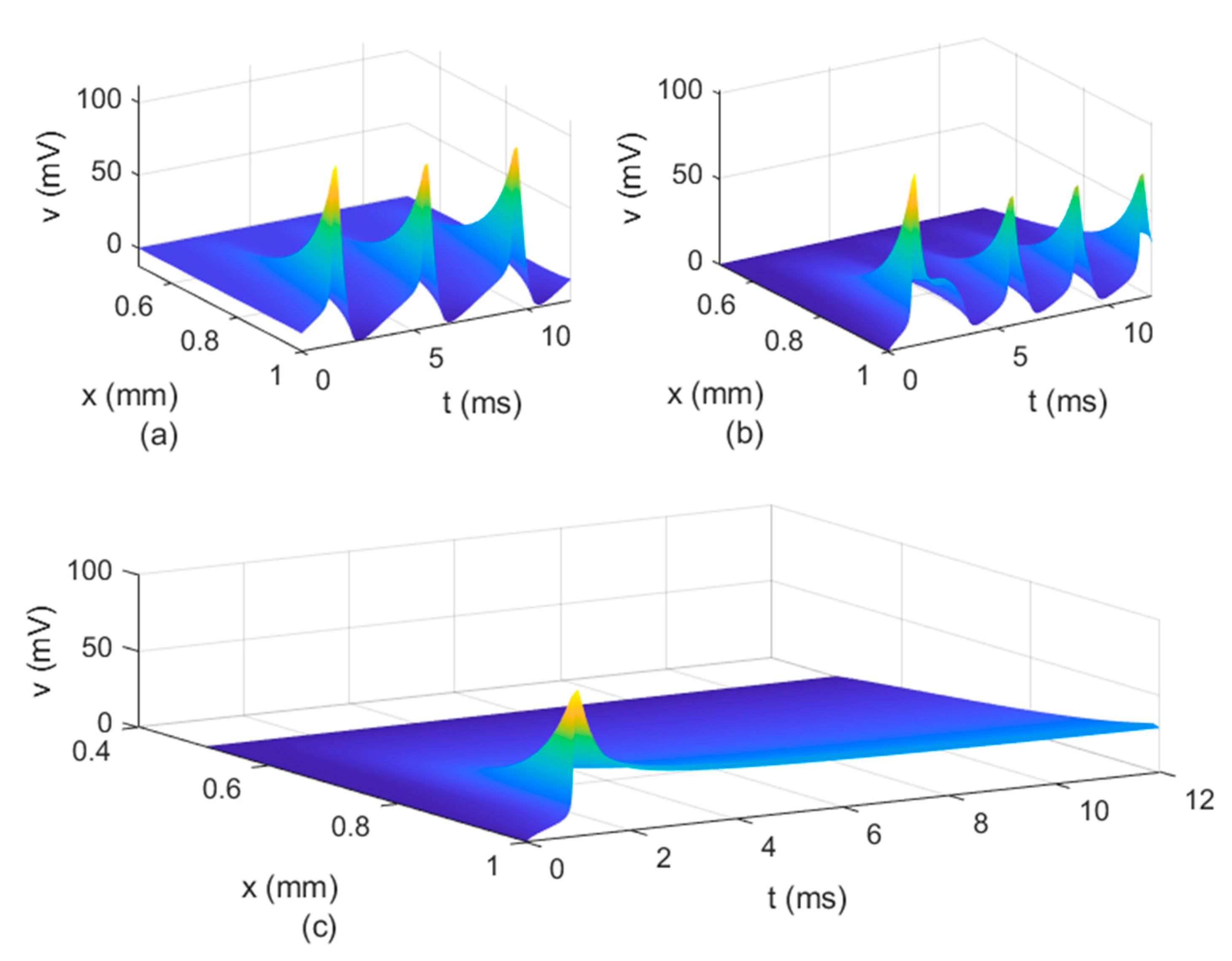
Figure 8, Figure 9 and Figure 10 show the variations in $v\left(x,t\right), n\left(t\right), m\left(t\right),$ and $h\left(t\right)$ for $\alpha =0.65$, $p=0.25 \mathrm{and} q=0.75$, and various values of $\beta .$ The same results are obtained for $p=0.75 \mathrm{and} q=0.25$. Thus, Figure 6, Figure 7, Figure 8, Figure 9 and Figure 10 suggest that the bidirectional propagation has little to no effect on the shapes of the action potentials at the nodes of Ranvier. At the fixed time $t=0.1 \mathrm{ms}$, the amplitude of the action potential at the node of Ranvier increases as the long-term memory increases (corresponding to $\beta$ decreasing) and its shape becomes wider (Figure 8a), while at fixed location $x=700 \mathsf{\mu }\mathrm{m}$ the potentials flatten with decreasing $\beta$ (Figure 8b). As the long-term memory increases, the delay in the opening and closing of the ion channels increases (Figure 9a–c) until they stop operating at $\beta =0.66$ (Figure 9d). Figure 8b shows that the potential reaches a steady state value at $\beta =0.66$. The spatio-temporal variations of $v\left(x,t\right)$ in Figure 10 show how possible defects in the membrane potentials start to develop as $\beta$ decreases. The increasing delay in the action potentials at the node of Ranvier with decreasing $\beta$ (Figure 10b) looks like the shapes of the membrane potentials observed experimentally in transgenic Na_v1.8-null knockout DRG neurons ([21], Figures 8b and 9c). Abnormal Na_v1.8 expression in some neurons may be linked to multiple sclerosis in humans [22]. Mutations of some sodium channels can cause persistent sodium currents that, combined with the blockade of potassium and calcium currents, lead to prolonged plateau potentials in the neurons of mice [25] (also [24], Figure 1B). These potentials resemble the ones in Figure 10b. According to [24], persistent sodium currents are linked to epilepsy. The same shape of the membrane potential shown in Figure 10b was also observed experimentally in neurons under spreading depolarization (SD) and a blockade of astrocytic glutamate transporters ([26], Figure 8a–c). SD occurs in traumatic brain injuries and ischemic stroke. Lastly, cerebral anoxic depolarization that happen during a stroke or brain ischemia causes a potential like the one in Figure 10c [23]. Without immediate treatment, this condition leads to brain death. Therefore, there is no physiological justification to further decrease the value of $\beta$. Nevertheless, it was observed that the solution becomes unstable for $\beta <0.63.$

In conclusion, the spatial non-locality controls the width of action potentials at the nodes of Ranvier, the narrower shapes being closer to the action potentials observed experimentally. The spatial parameters $p$ and $q$ control the strength of the forward and backward propagations of the action potentials; the weaker the forward propagation is, the lower the amplitude of the action potentials becomes. Lastly, the long-term memory in the presence of spatial non-locality could delay or stop the propagation of action potentials and widen the shapes of the action potentials at the nodes of Ranvier.

5. Conclusions

In this paper, it was assumed that the anomalous diffusion of ions and water through the myelin sheath, nodes of Ranvier and ECS affect the propagation of action potentials in myelinated neurons. A spatio-temporal fractional cable equation is proposed to model the effects of the long-range interactions and long-term memory of ions on the bidirectional propagation of action potentials in myelinated neurons. Caputo fractional derivatives and their properties were used to derive the equation. Numerical simulations showed the spatio-temporal distributions of the membrane potential in a leaky internodal region with one isopotential node described by the fractional Hodgkin–Huxley equations. The main finding is that the spatially wider shapes of the action potentials at the nodes of Ranvier and lack or delayed action potentials caused by the long-term memory combined with spatial non-locality could signal the presence of certain pathological conditions. Future work will explore possible effects on the propagation of action potentials of a time-dependent, non-local parameter $\alpha \left(t\right),$ and the interplay between $\alpha \left(t\right)$ and $\beta .$