Cole-Impedance Model Representations of Right-Side Segmental Arm, Leg, and Full-Body Bioimpedances of Healthy Adults: Comparison of Fractional-Order

Abstract

The passive electrical properties of a biological tissue, referred to as the tissue bioimpedance, are related to the underlying tissue physiology. These measurements are often well-represented by a fractional-order equivalent circuit model, referred to as the Cole-impedance model. Objective: Identify if there are differences in the fractional-order ($\alpha$) of the Cole-impedance parameters that represent the segmental right-body, right-arm, and right-leg of adult participants. Hypothesis: Cole-impedance model parameters often associated with tissue geometry and fluid ($R_{\infty }$, $R_1$, C) will be different between body segments, but parameters often associated with tissue type ($\alpha$) will not show any statistical differences. Approach: A secondary analysis was applied to a dataset collected for an agreement study between bioimpedance spectroscopy devices and dual-energy X-ray absoptiometry, identifying the Cole-model parameters of the right-side body segments of $N=174$ participants using a particle swarm optimization approach. Statistical testing was applied to the different groups of Cole-model parameters to evaluate group differences and correlations of parameters with tissue features. Results: All Cole-impedance model parameters showed statistically significant differences between body segments. Significance: The physiological or geometric features of biological tissues that are linked with the fractional-order ($\alpha$) of data represented by the Cole-impedance model requires further study to elucidate.

1. Introduction

The Cole-impedance expression, introduced by Kenneth Cole in 1940 [1], is an electrical impedance that has been widely utilized to represent the frequency-dependent electrical impedance of biological tissues. Recently, this expression (or equivalent circuit model representations of it) have been applied to model the frequency dependent impedance of human biceps tissues [2,3], skeletal muscle of mice [4], rabbit tissues [5], rat tissues [6], skin-electrode impedance [7], and modeling pork tissues during storage [8]. While these works are not an exhaustive summary of research that has employed the Cole-impedance expression (or equivalent circuit models), this subset does highlight efforts that employ this model to represent the electrical impedance of human and animal tissues. The original expression presented by Cole [1] is given by:

$$z=z_{\infty }+\frac{(r_0-r_{\infty })}{1+{\left(j\omega \tau \right)}^{\alpha }}$$

(1)

where $r_0$ and $r_{\infty }$ are described by Cole as the resistances at zero and infinite frequency, $\tau$ is the time constant of the suspension and $\alpha$ a variable related to the membrane impedance (and that it varies as some power of the frequency) [1]. It is possible to represent (1) using the electrical equivalent circuit given in Figure 1a. This equivalent circuit will be referred to as the Cole-impedance model throughout this manuscript and is composed of three circuit elements ($R_{\infty }$, $R_1$, and a constant phase element (CPE)). The impedance of this model is given by:

$$Z=R_{\infty }+\frac{R_1}{1+{\left(j\omega \right)}^{\alpha }{R}_{1}C}=R+jX$$

(2)

where R and X represent the resistance and reactance (in Ohms) of the impedance, which are often used to plot impedance datasets. Comparing the original impedance expression from Cole given by (1) with the circuit model impedance given by (2), these expressions are equivalent when: $z_{\infty }=r_{\infty }=R_{\infty }$, $r_0-r_{\infty }=R_1$, and $\tau ={\left(R_{1}C\right)}^{\frac{1}{\alpha }}$. While resistors are one of the traditional circuit elements commonly used in modeling impedance (in addition to inductors and capacitors), the CPE is not. A CPE is a theoretical circuit element that has the current-voltage characteristics given by:

$$i\left(t\right)=C\frac{d^{\alpha }v\left(t\right)}{d{t}^{\alpha }}$$

(3)

where $0<\alpha <1$ is the order of the CPE (and order of the fractional-order differentiation). Beyond the Cole-impedance model, CPEs have been utilized in modeling the mechanical impedance of lungs [9], the electrical impedance of lithium-ion batteries [10], and the electrical impedance of concrete [11].

The current-voltage relationship given by (3) is a fractional-order differential equation. This places the CPE component into the realm of fractional calculus, the mathematical field concerning integrals and derivatives of noninteger orders [12]. Concepts from this field are being imported and investigated for modeling biological phenomena as it offers methods to represent biological data using models with fewer parameters than integer-order models [13,14]. For reference, the Grunwald–Letnikov definition of a fractional derivative of order $\alpha$ is given by [15]:

$$D^{\alpha }f\left(x\right)=\underset{h\to 0}{lim}\sum _{m=0}^{\infty }\frac{{(-1)}^m}{h^{\alpha }}\frac{\Gamma (\alpha +1)}{m!\Gamma (\alpha -m+1)}f(x-mh)$$

(4)

where $D^{\alpha }$ is the unified notation developed by Harold T. Davis to describe the order of the differentiation or integration [16] (with further contemporary details available from Ross [17]) and $\Gamma (·)$ is the gamma function. Returning to the CPE, it has an electrical impedance $Z_{CPE}=1/C{\left(j\omega \right)}^{\alpha }$, where C and $\alpha$ are the pseudo-capacitance and fractional-order, respectively. With the fractional-order fixed in the interval $0<\alpha <1$ (common for biological tissues), the CPE has electrical characteristics that place it between a resistor ($\alpha =0$) and an ideal capacitor ($\alpha =1$). It is for this reason that a CPE (with this limited band of fractional-order) is also called a fractional-order capacitor. This reference to a fractional-order capacitor is why it is represented using a capacitor symbol in Figure 1. The units of a CPE/fractional-order capacitor proposed by Westerlund and Ekstam are $\mathrm{F}·{\sec }^{\alpha -1}$ [18], though often CPE units are presented in Farads. A simulation of (2) with parameters $R_{\infty }=100$ $\Omega$, $R_1=50$ $\Omega$, $C=10$ $\mu \mathrm{F}·{\sec }^{\alpha -1}$, and $\alpha =0.7,0.85,1$ are given in the Nyquist plot of Figure 1b. These specific values are selected because they are representative of values reported for segmental tissues in this work (but this will be explored later sections). Notice on an Nyquist plot, that this model has a semicircular behavior with the low and high frequency reactance approaching 0 $\Omega$ and that the maximum reactance of the semicircle is depressed for increasing values of $\alpha$. Each of these simulations approaches 100 $\Omega$ (the $R_{\infty }$ value) at high frequencies which is why this component is referred to as the high-frequency resistor. In addition, the simulations approach 150 $\Omega$ at low frequency (the $R_{\infty }+R_1$ value) highlighting that both resistors are related to the low-frequency behavior.

Recently this model has been used to represent the impedance of localized biceps tissues of healthy adults before/after exercise in the frequency band from 10 kHz to 100 kHz [2,3]. The aim of these efforts was to determine if the Cole-impedance model parameters of localized tissues are altered as a result of exercise, which would support their use as a reduced feature set for tissue monitoring over large datasets of raw impedances. In their work, Freeborn and Fu reported statistically significant decreases in the resistance parameters ($R_{\infty }$, $R_1$) but not the CPE parameters (C, $\alpha$) comparing the pre-exercise and post-exercise measurements [2]. In a further study of bicep tissue changes resulting from eccentric exercise, Fu and Freeborn reported statistically significant decreases in the resistance parameters ($R_{\infty }$, $R_1$) and increases in C (but no changes in $\alpha$) at timepoints 72 h and 96 h after the eccentric exercise stimulus [3]. Of interest in both studies from a fractional-order circuit model perspective, is that the fractional-order $\alpha$ did not show statistically significant differences as a result of either exercise protocol and that localized biceps tissues (expected to be composed primarily of skeletal muscle) had similar $\alpha$ (approximately $0.75$). Similar values were also reported by Regaud et al. for the CPE order of skeletal muscle from sheep ($0.71$) [19]. Based on the similar values of $\alpha$ between these studies, Fu and Freeborn hypothesized that the fractional-order may be linked to the tissue type (but this hypothesis was not tested).

This provides the motivation for this work, to compare the Cole-impedance model parameters that represent different segmental and full-body impedance measurements of healthy adults. This study has a particular focus on the CPE parameters (C, $\alpha$). It is hypothesized that parameters linked to tissue geometry and fluid ($R_{\infty }$, $R_1$, C) will be different between body segments, but parameters linked to tissue type ($\alpha$) will not show any statistical differences. To test this hypothesis, a secondary analysis of measurements collected/reported by Esco et al. in [20] was conducted. This dataset was collected during the course of an agreement study between bioimpedance spectroscopy devices and dual-energy X-ray absoptiometry for body composition determination [20] (but an investigation of the Cole-model parameters was not within its scope). From this dataset, the Cole-impedance parameters ($R_{\infty }$, $R_1$, C, $\alpha$) that represent the segmental tissue impedance of the right-side full body, right arm, and right leg of 176 adult participants were identified using a particle swarm optimization approach. These identified Cole-impedance parameters were then analyzed using statistical tests to identify if there are significant differences between parameters of different body segments. Finally, follow-up analyses to quantify correlations between Cole-impedance parameters and dual-energy X-ray absorptiometry (DXA) measures of soft tissues (tissue percent body fat) for these body segments were completed. Based on these results, while $R_{\infty }$ and C parameters show strong correlations with segmental lean tissue mass, the fractional-order ($\alpha$) of the Cole-impedance parameters does not show statistically significant correlations. The following sections of this work detail the methods to collection the bioimpedance datasets, methods for their analysis and comparison, the overall study results, and discussions of the results and their implications.

2. Materials and Methods

2.1. Study Participants

The data analyzed in this study was collected by the Exercise Physiology Lab research group at the University of Alabama (UA), a subset of which was previously reported by Esco et al. [20] for their agreement study between bioimpedance spectroscopy devices and DXA for body composition determination. Complete details of the data collection process are available in [20] but are also summarized here for easy reference.

During data collection, electrical impedance measurements and body composition measurements were collected using a bioimpedance spetroscopy and a DXA device, respectively. For this study, segmental measurements of the right arm, right leg, and right-side full body of 185 participants ($31.5\pm 14.8$ years, $170.8\pm 8.9$ cm, $76.6\pm 18.5$ kg) were analyzed. Measurements using both devices were collected from participants while in a supine body position after having arrived at the Exercise Physiology Lab at the University of Alabama in a fasted (8–12 h) euhydrated state. Additionally, participants were to have avoided strenuous exercise in the day prior to testing. This study was reviewed and approved by the institutional review board of The University of Alabama (15-019-ME). All study participants reported no cardiovascular or metabolic disease and were not pregnant. Each participant provided their written informed consent prior to data collection.

2.2. Dual-Energy X-ray Absorption Measurements

Dual-energy X-ray absorptiometry is a measurement method that utilizes the differences in absorption of X-ray photons at high and low energy to quantify bone and soft tissue. Further technical details regarding this technique are available from Pietrobelli et al. [21] for interested readers. DXA measurements of total tissue mass, fat tissue mass, and lean tissue mass of each body segment (right arm, right leg, right-side full body) were collected from each participant using a commercially available Lunar Prodigy Advance device from GE Healthcare. This system provides the hardware and software necessary to collect body composition assessments from a participant placed on the scanning bed. For this study, whole body scans were completed while participants were on the scanning bed of the device in a supine position with hands at their side and velcro straps wrapped at the ankles and knees. After the whole-body scan, the DXA tissue measurements reported by the device software were manually recorded for later analysis.

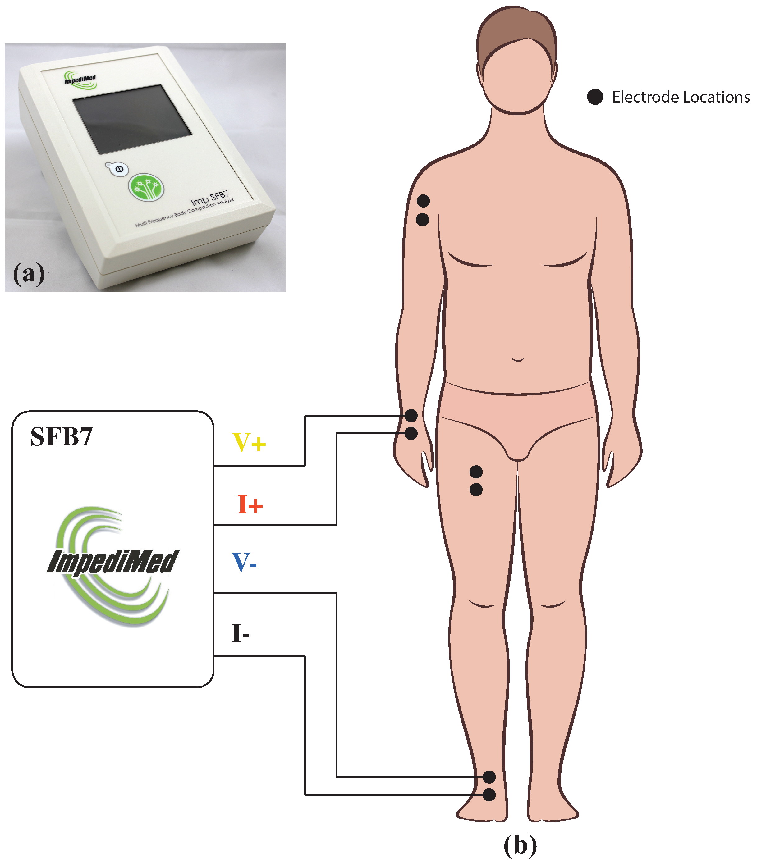
2.3. Electrical Impedance Measurements

The electrical impedance measurements of each body segment (right arm, right leg, right-side full body) were collected from each participant using a tetrapolar electrode configuration with an ImpediMed SFB7 device (shown in Figure 2a). The SFB7 is a commercially available instrument marketed by ImpediMed for the estimation of body composition in healthy individuals but is also widely utilized for clinical research [22,23]. This instrument measures impedances at 256 discrete frequencies from 3 kHz to 1 MHz, with a manufacturer rated accuracy of $1\%$ (for impedances as low as 10 $\Omega$); which has been validated by Freeborn et al. [24]. The SFB7 uses a tetrapolar configuration of electrodes, with two electrodes injecting the excitation current (I+, I−) and two electrodes measuring the voltage response of the tissue segment (V+, V−). A tetrapolar configuration is utilized to reduce (but cannot remove) the effects of the electrode/tissue interface impedance which is typically much larger than the tissue impedance. For further details regarding tetrapolar measurements, readers are recommended to review the works of Grimnes and Martinsen [25] and Aliau-Bonet and Pallas-Areny [26].

The approximate locations of the electrodes for each body segment measured in this study are detailed in Figure 2b. Electrodes were placed on the hand and shoulder, foot and thigh, and hand and foot for the right arm, right leg, and right-side full body measurements, respectively. For data collection in this study, adhesive Ag/AgCl electrodes were placed by the study personnel on each of the body sites after cleaning with isopropyl alcohol and removal of hair to improve contact with the skin. After electrode placement, participants were asked to lay supine while their electrical impedance measurements were collected using the SFB7 device interfaced to the electrodes. The cables of the SFB7 were manually attached to the necessary electrode pairs for each measurement. Figure 2b illustrates the connection of the SFB7 to the electrodes for the right-side full body measurement of a participant. Measurements from each of the 3 body segments were saved on the instrument for later download/post-processing in their raw format.

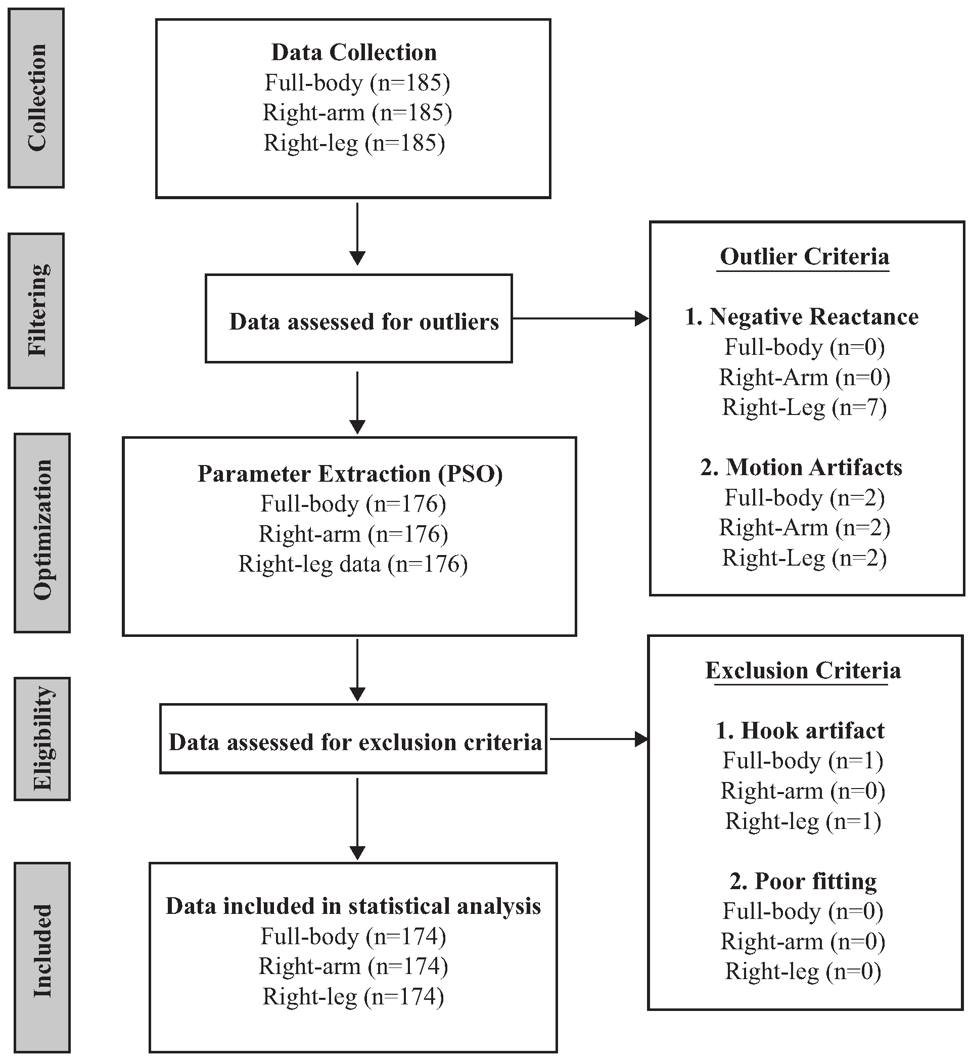
2.4. Outlier Identification/Removal

Before application of an optimization fitting procedure to identify the Cole-impedance model parameters that best represented each individual impedance dataset (described further in Section 2.5), the datasets were visually reviewed by the study team to identify if they had features that would prevent their fitting. The features that were screened in this step were negative reactances in the impedance plot at high frequency and motion artifacts. Samples of these types of features in sample impedance datasets are given in Figure 3b,c respectively. These artifacts are associated with errors in measurements and not representative of the tissue. A total of 7 negative reactance cases (all present in right-leg impedance datasets) and 2 cases of motion artifacts were identified. Note, because of the statistical testing utilized later in this work (described in Section 3.1), all datasets from a participant were excluded for those with a case of negative reactance or motion artifacts. Therefore, a total of 9 participants datasets were removed from the analysis at this stage. After parameter identification, the data was further analyzed for high-frequency hook artifact or a poor fitting, both determined by visual inspection. Two datasets were identified as having a hook artifact or poor fitting, shown in Figure 3a for reference. After this outlier identification/removal, the datasets of $N=174$ participants were used in the statistical analysis. This process of outlier identification is summarized in Figure 4.

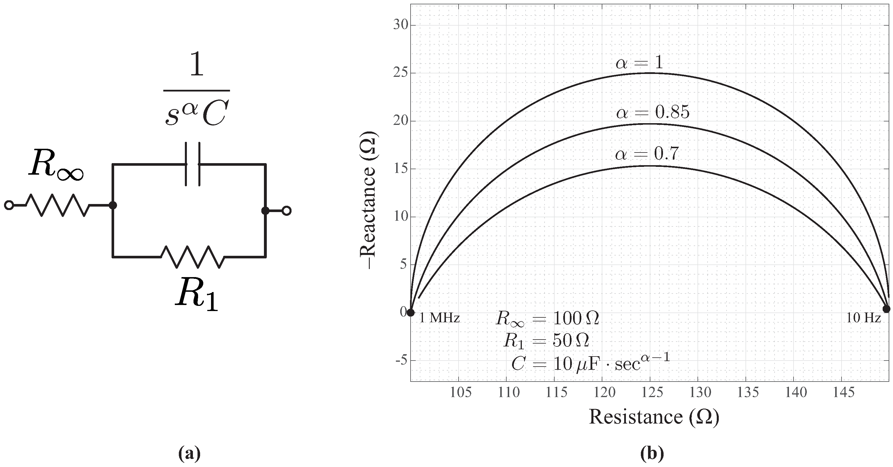
2.5. Cole-Impedance Model Parameter Identification

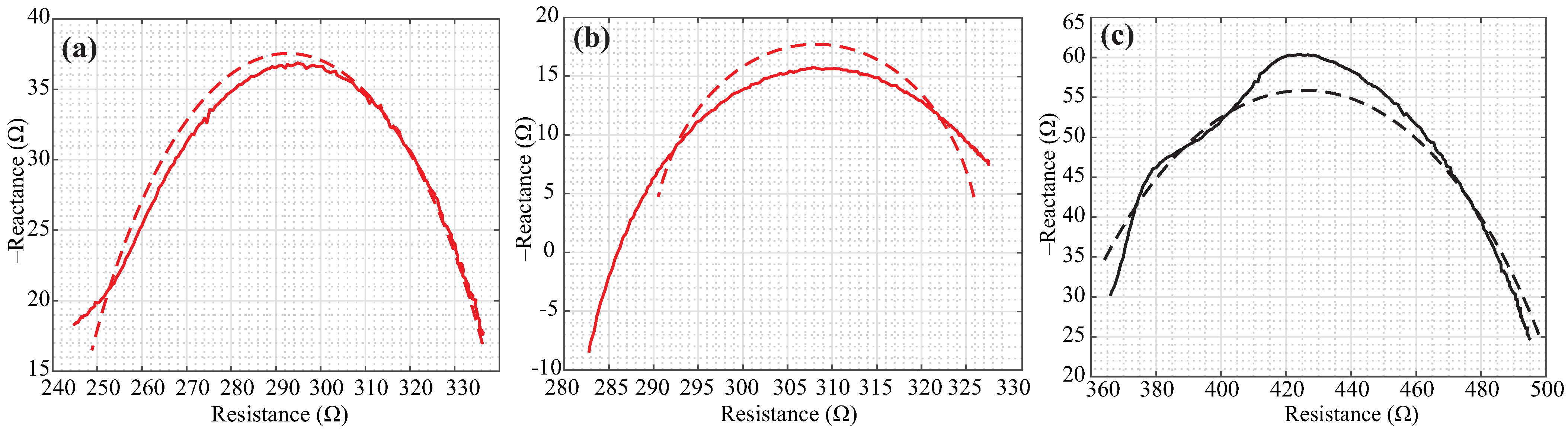
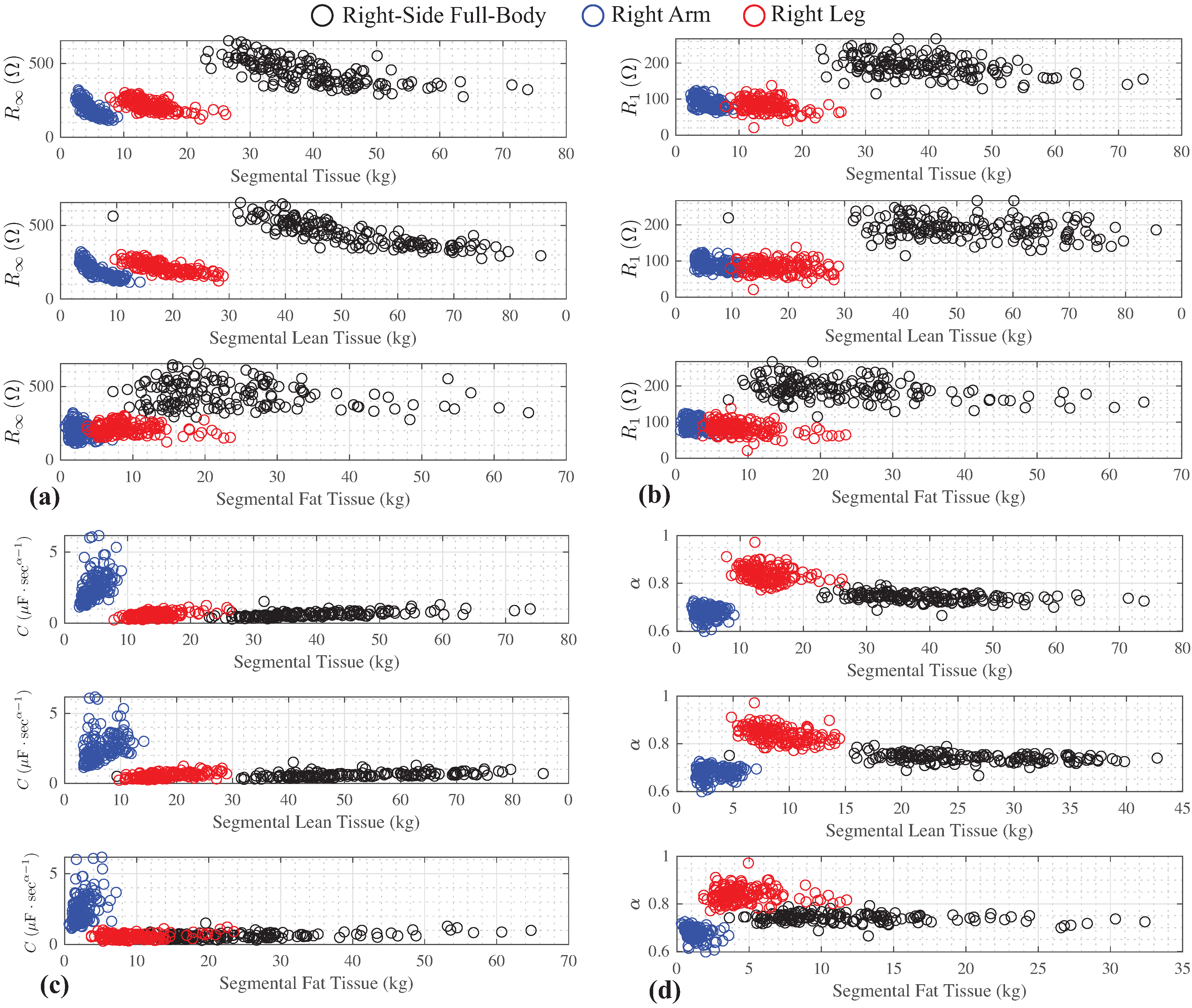
For each collected bioimpedance measurement, the Cole-impedance model parameters ($R_{\infty }$, $R_1$, C and $\alpha$) were extracted by applying a particle swarm optimization (PSO) to identify the parameters that minimized the squared difference (of the real and imaginary impedance components) between the experimental data (from 3 kHz to 200 kHz) and the Cole impedance model. Metaheuristic optimization procedures, such as PSO, have been previously utilized for estimating bioimpedance parameters from impedance datasets showing accurate results [27,28]. Based on the accuracy of the PSO implementations reported by Narango-Hernandez et al. for fitting bioimpedance data [28] and the ease of implementation using available MATLAB functions, this approach was adopted in this work. The objective function for the PSO optimization applied in this work is:

$$\underset{\mathit{x}}{min}{f}_0\left(\mathit{x}\right)=\sum _{k=1}^n{\left(\mathrm{Re}\{Z_k\left(\mathit{x}\right)-y_k\}\right)}^2+{\left(\mathrm{Im}\{Z_k\left(\mathit{x}\right)-y_k\}\right)}^2$$

(5)

where $f_0\left(x\right)$ is the objective function, n is the number of discrete frequencies used for fitting, $y_k$ is the collected electrical impedance impedance at the $k$-th frequency, $Z_k\left(x\right)$ is the impedance of the Cole impedance model with x (the vector of the model parameters $R_{\infty }$, $R_1$, C, $\alpha$), and $\mathrm{Re}$ and $\mathrm{Im}$ denote the real and imaginary components of the impedances. This procedure was implemented using the particleswarm function available in MATLAB with the following options: Swarm Size$=1000$, Social Adjustment Weight $=1$, MinNeighborsFraction $=0.6$, and the hybrid functionality was enabled to apply the fmincon solver after the PSO solver terminated. Hybrid functions can obtain a more accurate solution (to the PSO alone) by starting from the relatively rough solution found by the first solver. This functionality is built into the MATLAB functions to implement the PSO and does not require additional effort on the part of the user to setup. Constraints were also added to the PSO implementation, with lower and upper boundaries for $\left[R_{\infty },R_1,C,\alpha \right]$ fixed at $\left[1\mathrm{m}\Omega ,1\mathrm{m}\Omega ,1\mathrm{nF}·{\sec }^{\alpha -1},0.5\right]$ and $\left[100\Omega ,100\Omega ,0.1\mathrm{mF}·{\sec }^{\alpha -1},1.05\right]$, respectively.

3. Results

A sample of participant impedances with simulations using the PSO identified Cole-model parameters are given in Figure 5 for 6 different participants. In each of the subfigures, the solid lines represent the experimental data and dashed lines represent the MATLAB simulated Cole-impedance using (2). The line color is used to differentiate the body segments with black, red, and blue corresponding to the right-side full-body, right-arm, and right-leg data, respectively. Notice that each dataset, regardless of body segment has an arc which is well-represented by the simulation using the Cole-impedance model (and appropriate model parameters). To highlight the effect that outlier datasets have on the PSO identification process, simulations using identified Cole-impedance parameters from previously removed hook artifact data, positive reactance, and motion artifacts are shown in Figure 3. In each case, the simulations shown as dashed lines show a significant deviation compared to the experimental measurements (solid), indicating that the Cole-impedance model is a poor fit when these artifacts are present.

To visualize the complete range of the set of Cole-impedance model parameters that were identified from all participant datasets, histograms of $R_{\infty }$, $R_1$, C, and $\alpha$ are detailed in Figure 6. From these figures, there is significant overlap between the right arm and right leg $R_{\infty }$ and $R_1$ parameters and very little overlap between right arm/leg and right-side full body parameters. The $R_{\infty }$ values range from approximately 100 $\Omega$ to 200 $\Omega$ for right arm/leg and 300 $\Omega$ and 600 $\Omega$ for right side full-body. $R_1$ ranges from approximately 50 $\Omega$ to 125 $\Omega$ for right arm/leg and 150 $\Omega$ and 250 $\Omega$ for right side full-body. C is $<1$ $\mu$F for right leg/right side full-body and 1 $\mu$F to 6 $\mu$F for right arm. Of significant interest for this study, is that the fractional-order ($\alpha$) of the different body segments shows very little overlap. With the right arm values ranging from approximately $0.6$ to $0.73$, full body values ranging from $0.73$ to $0.8$, and right leg values ranging from $0.8$ to $0.9$. The median values of the Cole-impedance model parameters from the complete set of extracted values from the 174 participants are given in

Table 1. Median Cole-impedance model parameters ($R_{\infty }$, $R_1$, C, $\alpha$) identified by the PSO to best-fit the 174 participant right-side full body, right arm, and right leg bioimpedance datasets.

Body Segment	${\mathit{R}}_{\mathit{\infty }}$ ($\mathbf{\Omega }$)	${\mathit{R}}_1$ ($\mathbf{\Omega }$)	C$\mathsf{\mu }\mathbf{F}·{\mathbf{sec}}^{\mathit{\alpha }-1}$	$\mathit{\alpha }$
Right-side Full Body	$440.28$	$191.32$	$0.566$	$0.7428$
Right Arm	$191.39$	$92.51$	$2.57$	$0.6841$
Right Leg	$210.56$	$80.05$	$0.534$	$0.8374$

.

3.1. Statistical Testing: Friedman Test

To test the study hypothesis (that the fractional-order, $\alpha$, for each body segment will be equal) statistical testing was utilized to compare the Cole-impedance impedance parameters obtained from each body segment. Prior to the statistical comparison, the normality of the parameters datasets were tested using the Shapiro–Wilk’s test ($p<0.05$). The assumption of normality for $\alpha$ for the full-body and right-arm segments were violated but not for the right-leg. The assumption of normality for $R_{\infty }$ values were satisfied for the right-leg dataset but not for the full-body and right-arm. The assumption of normality for $R_1$ values were satisfied for the full-body and right-leg but not the right-arm. Lastly, the assumption of normality for C values were not satisfied for all body locations. Because some groups within our dataset violated normality and were not independent, the nonparametric Friedman test was utilized to determine if there were statistically significant differences between the 3 related samples groups.

For the applied Friedman test (SPSS Statistics 26) statistical significance was accepted at the $p<0.05$ level. The medians for each set of parameters in this analysis are detailed in Table 1. From the Friedman test, the fractional order ($\alpha$) was statistically different for all segments, ${\chi }^2\left(2\right)=346.011, p<0.005$. From similar tests the $R_{\infty }$, $R_1$, and C parameters were statistically different for all segments ($R_{\infty }:{\chi }^2\left(2\right)=292.08, p<0.005$; $R_1:{\chi }^2\left(2\right)=275.89, p<0.005$; $C:{\chi }^2\left(2\right)=269.38, p<0.005$). Following each analysis, pairwise comparisons were performed with a Bonferroni correction for multiple (3) comparisons. For each parameter ($R_{\infty }$, $R_1$, C, $\alpha$) there were statistically significant differences ($p<0.0167$) for the right-arm/right-leg, right-arm/right-body, and right-leg/right-body comparisons.

3.2. Statistical Testing: Spearman Correlation

To determine if there were correlations (and their strengths) between the Cole-impedance parameters and total tissue/tissue type, Spearman’s rank-order correlation coefficients were calculated in MATLAB between each of the parameters ($R_{\infty }$, $R_1$, C, $\alpha$) for each body segment and the DXA calcualted total tissue, lean tissue, and fat tissue (each in kg). The scatterplots of these datasets are given in Figure 7. In each subplot, Figure 7a–d, there are three scatterplots to visualize each of the Cole parameters with the segmental tissue mass, segmental lean mass, and segmental fat mass for that body segment. Each body segment is represented by a different color, with black/blue/red representing the right-side full-body/right arm/right leg, respectively. Note that only 159 of the 174 participants with identified Cole-impedance model parameters had available DXA data for this analysis.

The Spearman-rank correlation coefficients ($r_s$) and their corresponding statistical significance (if $p<0.05$) are presented in

Table 2. Spearman-rank correlation coefficients ($r_s$) and statistical significant (p) between Cole-impedance parameters and total/lean/fat tissue masses for segmental measurements.

	Total Tissue (kg)			Lean Tissue (kg)			Fat Tissue (kg)
	Full-Body	Arm	Leg	Full-Body	Arm	Leg	Full-Body	Arm	Leg
$R_{\infty }$ ($\Omega$)
$r_s\left(157\right)$	$-0.731$	$-0.856$	$-0.641$	$-0.862$	$-0.903$	$-0.781$	−	−	−
p	<0.001	<0.001	<0.001	<0.001	<0.001	<0.001	−	−	−
$R_1$ ($\Omega$)
$r_s\left(157\right)$	$-0.375$	$-0.528$	$-0.222$	$-0.267$	$-0.517$	−	$-0.323$	−	$-0.307$
p	<0.001	<0.001	$0.020$	$0.003$	<0.001	−	<0.001	−	<0.001
C ($\mu \mathrm{F}·{\sec }^{\alpha -1}$)
$r_s\left(157\right)$	$0.682$	$0.636$	$0.542$	$0.612$	$0.545$	$0.611$	$0.334$	$0.366$	−
p	<0.001	<0.001	<0.001	<0.001	<0.001	<0.001	<0.001	<0.001	−
$\alpha$
$r_s\left(157\right)$	$-0.384$	−	$-0.334$	$-0.351$	−	$-0.468$	−	$-0.386$	−
p	<0.001	−	<0.001	<0.001	−	<0.001	−	<0.001	−

Note: A blank cell (“–”) indicates no statistically significant correlation.

. Coefficients that were not statistically significant are not reported. For the calculation of the statistical significance, a Bonferroni correction was applied to compensate for the multiple correlations (4) per segmental dataset. As an example of using Table 2, there was a statistically significant, moderate negative correlation between total tissue mass of the right-side full-body and the $R_{\infty }$ Cole-impedance parameter ($p<0.001$, $r_s=-0.731$), a very strong negative correlation between lean tissue mass of the right-side full-body and $R_{\infty }$ ($p<0.001$, $r_s=-0.862$), and no statistically significant correlation between fat tissue mass and $R_{\infty }$.

4. Discussion

The results of the statistical analysis support that $R_{\infty }$, $R_1$, and C parameters of the Cole-impedance model to represent the 3 body segments measured in this study are in fact different. This aligns with the study hypothesis, that body segments with different dimensions would have different $R_{\infty }$, $R_1$, and C. The magnitude of differences also aligns with expectations based on segmental dimensions. That is, the resistances ($R_{\infty }$, $R_1$) for the right-side full-body measurements have a median value that is more than $2x$ the values of the right arm and leg values (medians given in Table 1). The full-body measurements capture tissues and fluids of the arm, leg, and torso which represents a greater resistive path to the excitation current injected by the electrodes than the arm/leg alone and are expected to be a major contribution towards these differences. This trend of increasing resistance with increasing distance between electrodes also aligns with previous forearm impedance measurements reported by Fu and Freeborn [29].

The moderate to strong correlations of $R_{\infty }$ with lean tissue mass in Table 2 aligns with previous bioelectrical impedance studies to estimate skeletal muscle mass [30,31]. The resistance measurement (either from a single frequency or the Cole-model estimated value) is typically used as a variable in estimation equations for skeletal muscle and fat free mass. As an example, Janssen et al. reported the following regression equation for skeletal muscle mass (SM) in kg given by:

$$\mathrm{SM}=\left[\frac{{\mathrm{Ht}}^2}{R}\times \left(0.401\right)+\mathrm{gender}\times \left(3.825\right)+\mathrm{age}\times (-0.071)\right]+5.102$$

(6)

where Ht is height (in cm), R is 50 kHz resistance (in $\Omega$), gender is a binary variable (men = 1, women = 0), and age is in years [30]. Notice in (6) that R is in the denominator of the Ht${}^2/R$ term, which will reduce this terms contribution to the estimated skeletal muscle mass for larger values of R. This is consistent with other reported regression equations to estimate lean tissue mass [31]. The reported results in this work also align with this trend, with lower resistance values being correlated with higher DXA estimated lean tissue mass.

The most significant result of this work is that the statistical comparison of the $\alpha$ values in Figure 6 between segmental/full-body electrical impedance does not support the study hypothesis. The initial hypothesis, that the value $\alpha$ would be strongly associated with tissue type (skeletal muscle) and not have statistically significant differences between the values identified for the different measured body segments of the study participants is not supported. Based on the statistical comparison the median $\alpha$ for the right side full body, arm, and leg were not equal, with values of $0.7428$, $0.6841$, and $0.8374$, respectively. This corresponds to differences of approximately $-7.9\%$ and $12.7\%$ comparing the arm and leg median $\alpha$ to the full-body value.

In terms of interpreting these results, it is important to analyze the underlying assumptions of the initial study hypothesis, which are: (1) that segmental limb geometry does not have a significant impact on $\alpha$, and (2) segmental limb tissues were composed primarily of skeletal muscle. The availability of DXA derived values of lean tissue mass, fat mass, and bone mineral content for each participant provide the opportunity to explore the tissue composition assumption. To visualize tissue composition with DXA measurements the lean tissue, fat mass, and bone mineral content (BMC) as a percentage of the total body mass (for the right side body, right arm, and right leg) was generated and plotted in Figure 8. Each vertical bar represents a single participant, with orange, red, and blue used to represent the percentage to segmental/body composition of BMC, fat tissue, and lean tissue, respectively. The mean (±SD) contribution of lean tissue from right arm, leg, and body measurements are $69.5\%\pm 9.4\%$, $64.5\%\pm 8.3\%$, and $66.9\%\pm 8.4\%$. This supports that full body and segmental tissues are composed primarily of lean tissues/skeletal muscle. As a result, it is likely that the segmental limb geometry does in fact have a significant impact on $\alpha$.

To further explore recent reports of the fractional-order $\alpha$ of Cole-parameters estimated from localized or segmental tissues of humans and animals (and compare them to the results of this work), a summary of recent studies is provided in

Table 3. Summary of fractional-order ($\alpha$) reported from studies of skeletal muscle tissue impedance utilizing Cole-impedance model.

Authors	Sample Population	Muscle Location	Frequency Band	Fractional-Order ($\mathit{\alpha }$)
Rigaud et al. [19]	Sheep	Gemellus (Ex Vivo)	$7.2$ kHz–720 kHz	Longitudinal: $0.73\pm 0.05$ Traverse: $0.78\pm 0.02$
Arnold et al. [32]	Mice	Gastrocnemius (Surface)	1 kHz–10 MHz	Longitudinal (Young): $0.682$ Traverse (Young): $0.660$ Longitudinal (Aged): $0.794$ Traverse (Aged): $0.656$
Nagy et al. [33]	Mice	Gastrocnemius (Surface)	1 kHz–10 MHz	Longitudinal: $0.709$–$0.760$ Traverse: $0.713$–$0.748$
Clark-Matott et al. [34]	Mice	Gastrocnemius Ex Vivo	1 kHz–10 MHz	Longitudinal: $0.522$–$0.677$ Traverse: $0.690$–$0.784$
Sanchez, Bragos, & Rutkove [35]	Rat	Gastrocnemius (Ex Vivo) Soleus (Ex Vivo)	1 kHz–1 MHz 1 kHz–1 MHz	Longitudinal: $0.528\pm 0.012$ Traverse: $0.729\pm 0.01$ Longitudinal: $0.695\pm 0.02$ Traverse: $0.736\pm 0.01$
Freeborn & Fu [2]	Healthy Adults	Biceps (Surface)	10 kHz–100 kHz	Pre Exercise: $0.552$–$0.781$ Post Exercise: $0.552$–$0.779$
Fu & Freeborn [3]	Healthy Adults	Biceps (Surface)	10 kHz–100 kHz	Exercised: $0.621$–$0.745$ Unexercised: $0.628$–$0.766$
Sato et al. [36]	Healthy Men (Surface)	Lower Extremities	5 kHz–250 kHz	$0.71\pm 0.03$
This work	Healthy Adults	Right-Body, Segmental Arm/Leg	3 kHz–200	Right-Body: 0.687–0.769 Right Arm: 0.606–0.725 Right Leg: 0.778–0.971

. This table details the animal/human population from which measurements were collected, the muscle location (if available), the measurement approach (Ex Vivo or surface), frequency band of measurement, and the range of $\alpha$ that was reported. While the range of fractional-orders are all in the approximate range of $0.52<\alpha <0.97$, highlighting that a fractional-order model has provided good fit of experimental bioimpedance data, there is a significant overlap between $\alpha$ across the studies without any tight groupings for specific test conditions. For example, measurements of excised skeletal muscle tissue and exposed skeletal muscle tissue in animals have overlapping $\alpha$ compared to segmental surface measurements in animal/human populations. However, it is important to note that the measurements summarized from these studies all have significantly different setups and test populations; which includes different electrode spacing, tissue contributions, tissue geometry, sample populations, and underlying physiology. So while reports from literature support that a wide range of $\alpha$ values has been determined from lean tissues, it does not provide a clear answer regarding what features $\alpha$ may be linked.

While these results do not support the initial study hypothesis, they do highlight that continued research is needed to elucidate what physiological or geometric features of biological tissues are strongly linked with the fractional-order ($\alpha$) of data represented by the Cole-impedance model. Even though the Cole-impedance model continues to provide a good “fit” with experimental data, the potential insights that it can offer regarding skeletal muscle cannot be unlocked until this relationship is understood in greater detail. In fact, this supports previous concerns of McAdams and Jossinet, who have reported limitations and sources of error in using equivalent circuit modeling to represent the electrical properties of biological tissues [37], which they recommend only after extensive study of the system under different conditions. This recommendation should be adopted in future studies to investigate how $\alpha$ is modified in biological tissues under different conditions to further understand what conditions it is most strongly associated.

5. Conclusions

While the Cole-impedance model is a fractional-order circuit model that well represents the experimental impedance measurements of segmental body impedances (right-side full-body, right arm, and right leg), the fractional-order ($\alpha$) parameter of this model showed statistically significant differences comparing the segmental measurements of healthy adults reported in this study. This supports that the fractional-order ($\alpha$) is not strongly associated with tissue type (i.e., skeletal muscle) which warrants further research to elucidate the tissue features to which it is most strongly associated towards advancing understanding of this model and tissue bioimpedance.

References

1. Cole, K. Permeability and impermeability of cell membranes for ions. Cold Spring Harbor Symp. Quant. Biol. 1940, 8, 110–122. [Google Scholar] [CrossRef]
2. Freeborn, T.J.; Fu, B. Fatigue-induced cole electrical impedance model changes of biceps tissue bioimpedance. Fractal Fract. 2018, 2, 27. [Google Scholar] [CrossRef] [Green Version]
3. Fu, B.; Freeborn, T. Cole-impedance parameters representing biceps tissue bioimpednace in healthy adults and their alterations following eccentric exercise. J. Adv. Res. 2020, 25, 285–293. [Google Scholar] [CrossRef] [PubMed]
4. Sanchez, B.; Li, J.; Geisbush, T.; Bardia, R.; Rutkove, S. Impedance alterations in healthy and diseased mice during electrically induced muscle contraction. IEEE Trans. Biomed. Eng. 2016, 63, 1602–1612. [Google Scholar] [CrossRef]
5. Al-Surkhi, O.; Naser, R. Detection of cell morphological changes of ischemic rabbit liver tissue using bioimepdance spectroscopy. IEEE Trans. Nanobiosci. 2018, 17, 402–408. [Google Scholar] [CrossRef]
6. Parramon, D.; Erill, I.; Guimer, A.; Ivorra, A.; Munoz, A.; Sola, A.; Fondevila, C.; Garcia-Valdecasas, J.; Villa, R. In vivo detection of liver steatosis in rats based on impedance spectroscopy. Physiol. Meas. 2007, 28, 813–828. [Google Scholar] [CrossRef]
7. Taji, B.; Chan, A.; Shirmohammadi, S. Effect of Pressure on Skin-Electrode Impedance in Wearable Biomedical Measurement Devices. IEEE Trans. Instrumen. Meas. 2018, 67, 1900–1912. [Google Scholar] [CrossRef]
8. Bai, X.; Hou, J.; Wang, L.; Wang, M.; Wang, X.; Wu, C.; Yu, L.; Yang, J.; Leng, Y.; Sun, Y. Electrical impedance analysis of pork tissues during storage. Food Meas. 2018, 12, 164–172. [Google Scholar] [CrossRef]
9. Ribeiro, D.; Abrantes, J. Application of electrochemical impedance spectroscopy (EIS) to monitor the corrosion of reinforced concrete: A new approach. Constr. Build. Mater. 2016, 111, 98–104. [Google Scholar] [CrossRef]
10. Westerhoff, U.; Kurbach, K.; Lienesch, F.; Kurrat, M. Analysis of Lithium-Ion Battery Models Based on Electrochemical Impedance Spectroscopy. Energy Technol. 2016, 4, 1620–1630. [Google Scholar] [CrossRef] [Green Version]
11. Ionescu, C.; Tenreiro Machado, J.; De Keyser, R. Modeling of the Lung Impedance Using a Fractional-Order Ladder Network With Constant Phase Elements. IEEE Trans. Biomed. Circuits Syst. 2011, 5, 83–89. [Google Scholar] [CrossRef] [PubMed]
12. Podlubny, I. Fractional Differential Equations; Academic Press: Cambridge, MA, USA, 1998. [Google Scholar]
13. Freeborn, T.J. A survey of fractional-order circuit models for biology and biomedicine. IEEE J. Emerg. Sel. Top. Circuits Syst. 2013, 3, 416–424. [Google Scholar] [CrossRef]
14. Ionescu, C.; Lopes, A.; Copot, D.; Machado, J.T.; Bates, J. The role of fractional calculus in modeling biological phenomena: A review. Commun. Nonlinear Sci. Numer. Simul. 2017, 51, 141–159. [Google Scholar] [CrossRef]
15. Shantanu, D. Functional Fractional Calculus for System Identification and Controls; Springer: Berlin/Heidelberg, Germany, 2008. [Google Scholar]
16. Davis, H.T. The Theory of Linear Operators; Principia Press: Grand Rapids, MI, USA, 1936. [Google Scholar]
17. Ross, B. Fractional Calculus. Math. Mag. 1977, 50, 115–122. [Google Scholar] [CrossRef]
18. Westerlund, S.; Ekstam, L. Capacitor theory. IEEE Trans. Dielectr. Elec. Insul. 1994, 1, 586–839. [Google Scholar] [CrossRef]
19. Rigaud, B.; Hamzaoui, L.; Frikha, M.R.; Chauveau, N.; Morucci, J.P. In vitro tissue characterization and modelling using electrical impedance measurements in the 100 Hz–10 MHz frequency range. Physiol. Meas. 1995, 16, A15–A28. [Google Scholar] [CrossRef]
20. Esco, M.R.; Fedewa, M.V.; Freeborn, T.J.; Moon, J.R.; Wingo, J.E.; Cicone, Z.; Holmes, C.J.; Hornikel, B.; Welborn, B. Agreement between supine and standing bioimpedance spectroscopy devices and dual-energy X-ray absorptiometry for body composition determination. Clin. Physiol. Funct. Imaging 2019, 39, 355–361. [Google Scholar] [CrossRef]
21. Pietrobelli, A.; Formica, C.; Wang, Z.; Heymsfield, S. Dual-energy X-ray absorptiometry body composition model: Review of physical concepts. Am. J. Physiol. Endocrinol. Metab. 1996, 271, E941–E951. [Google Scholar] [CrossRef]
22. Pateyjohns, I.; Brinkworth, G.; Buckley, J.; Boakes, M.; Clifton, P. Comparison of three bioelectrical impedance methods with DXA in overweight and obese men. Obesity 2006, 14, 2064–2070. [Google Scholar] [CrossRef]
23. Vine, S.; Painter, P.; Kuskowski, M.; Earthman, C. Bioimpedance spectroscopy for the estimation of fat-free mass in end-stage renal disease. e-SPEN Eur. J. Clin. Nutr. Metab. 2011, 6, e1–e6. [Google Scholar] [CrossRef]
24. Freeborn, T.J.; Milligan, A.; Esco, M.R. Evaluation of ImpediMed SFB7 BIS device for low-impedance measurements. Measurement 2018, 129, 20–30. [Google Scholar] [CrossRef]
25. Grimnes, S.; Martinsen, O. Journal of Physics D: Applied Physics Sources of error in tetrapolar impedance measurements on biomaterials and other ionic conductors. J. Phys. D Appl. Phys. 2006, 20, 9–14. [Google Scholar]
26. Aliau-Bonet, C.; Pallas-Areny, R. On the Effect of Body Capacitance to Ground in Tetrapolar Bioimpedance Measurements. IEEE Trans. Biomed. Eng. 2012, 59, 3405–3411. [Google Scholar] [CrossRef] [PubMed]
27. Yousri, D.; AbdelAty, A.; Said, L.; AboBakr, A.; Radwan, A. Biological inspired optimization algorithms for cole-impedance parameters identification. Int. J. Electron. Commun. 2017, 78, 79–89. [Google Scholar] [CrossRef]
28. Naranjo-Hernandez, D.; Reina-Tosina, J.; Roa, L.; Barbarov-Rostan, G.; Areste-Fosalba, N.; Lara-Ruiz, A.; Cejudo-Ramos, P.; Ortega-Ruiz, F. Smart bioimpedance spectroscopy device for body composition estimation. Sensors 2020, 20, 70. [Google Scholar] [CrossRef] [Green Version]
29. Fu, B.; Freeborn, T. Estimating localized bio-impedance with measures from multiple redundant electrode configurations. In Proceedings of the 2018 40th Annual International Conference of the IEEE Engineering in Medicine and Biology Society, Honolulu, HI, USA, 17–21 July 2018; pp. 4351–4354. [Google Scholar]
30. Janssen, I.; Hymsfield, S.; Baumgartner, R.; Ross, R. Estimation of skeletal muscle mass by bioelectrical impedance analysis. J. Appl. Physiol. 2000, 89, 465–471. [Google Scholar] [CrossRef] [Green Version]
31. Kyle, U.; Bosaeus, I.; De Lorenzo, A.; Deurenberg, P.; Elia, M.; Gomez, J.; Heitmann, B.; Kent-Smith, L.; Melchior, J.; Pirlich, M.; et al. Bioelectrical impedance analysis—Part i: Review of principles and methods. Clin. Nutr. 2004, 23, 1226–1243. [Google Scholar] [CrossRef]
32. Arnold, W.; Taylor, R.; Li, J.; Nagy, J.; Sanchez, B.; Rutkove, S. Electrical impedance myography detects age-related muscle change in mice. PLoS ONE 2017, 12, e0185614. [Google Scholar] [CrossRef] [Green Version]
33. Nagy, J.; Kapur, K.; Taylor, R.; Sanchez, B.; Rutkove, S. Electrical impedance myography as a biomarker of myostatin inhibition with ActRIIB-mFc: A study in wild-type mice. Future Sci. OA 2018, 4, FSO308. [Google Scholar] [CrossRef] [Green Version]
34. Clark-Matott, J.; Nagy, J.; Sanchez, B.; Taylor, R.; Riveros, D.; Abraham, N.; Simon, D.; Rutkove, S. Altered muscle electrical tissue properties in a mouse model of premature aging. Muscle Nerve 2019, 60, 801–810. [Google Scholar] [CrossRef]
35. Sanchez, B.; Bragos, R.; Rutkove, S. Differentiation of the intracellular structure of slow- versus fast-twitch muscle fibers through evaluation of the dielectric properties of tissue. Phys. Med. Biol. 2014, 59, 2369–2380. [Google Scholar] [CrossRef] [PubMed]
36. Sato, H.; Nakamura, T.; Kusuhara, T.; Kenichi, K.; Kuniyasu, K.; Kawashima, T.; Hanayama, K. Effectiveness of impedance parameters for muscle quality evaluation in healthy men. J. Physiol. Sci. 2020, 70, 53. [Google Scholar] [CrossRef] [PubMed]
37. McAdams, E.; Jossinet, J. Problems in equivalent circuit modelling of the electrical properties of biological tissues. Bioelectrochem. Bioenerg. 1996, 40, 147–152. [Google Scholar] [CrossRef]
Figure 1. (a) Electrical circuit representation of the Cole-impedance expression [1] and (b) MATLAB simulated Nyquist plot of (2) with R = 100 Ω , R 1 = 50 Ω , C = 10 μ F · sec α 1 when α = 0.7 ,   0.85 ,   1 .
Fractalfract 05 00013 g001
Figure 2. (a) ImpediMed SFB7 device to collect participant electrical impedance using (b) referenced electrode locations to measure segmental right arm, segmental right leg, and right full-body of each study participant with tetrapolar configuration.
Fractalfract 05 00013 g002
Figure 3. Samples of participant data excluded (solid) from statistical analysis due to (a) high-frequency hook artifact, (b) positive high-frequency reactance, and (c) motion artifacts. Simulations using identified Cole-impedance parameters (dashed) shown to highlight poor fitting for datasets with these characteristics.
Fractalfract 05 00013 g003
Figure 4. Process applied to complete set of electrical impedance datasets for outlier identification/removal, resulting in the use of N = 174 participant datasets (from an original set of N = 185 ).
Fractalfract 05 00013 g004
Figure 5. Samples of right-side full-body (black), right arm (blue), and right leg (red) bioimpedances collected from participants (solid line) compared to simulations of Cole-impedance model using PSO identified parameters (dashed).
Fractalfract 05 00013 g005
Figure 6. Histograms of the Cole-impedance model parameters ( R , R 1 , C, α ) identified by the PSO to best-fit the participant right-side full body (blue), right arm (orange), and right leg (yellow) datasets.
Fractalfract 05 00013 g006
Figure 7. Scatterplots of (a) R , (b) R 1 , (c) C, and (d) α vs. total segmental tissue, lean tissue, and fat tissue for right-side full body (black), right arm (blue), and right leg (red) impedance datasets.
Fractalfract 05 00013 g007
Figure 8. DXA derived contributions of bone mineral content (orange), fat tissue (red), and lean tissue (blue) to overall composition of right arm, right leg, and right body of study participants.
Fractalfract 05 00013 g008