1. Introduction
A stochastic calculus of variations, which generalizes the ordinary calculus of variations to stochastic processes, was introduced in 1981 by Yasue, generalizing the Euler–Lagrange equation and giving interesting applications to quantum mechanics [
1]. Recently, stochastic variational differential equations have been analyzed for modeling infectious diseases [
2,
3], and stochastic processes have shown to be increasingly important in optimization [
4].
In 1996, fifteen years after Yasue’s pioneer work [
1], the theory of the calculus of variations evolved in order to include fractional operators and better describe non-conservative systems in mechanics [
5]. The subject is currently under strong development [
6]. We refer the interested reader to the introductory book [
5] and to [
7,
8,
9] for numerical aspects on solving fractional Euler–Lagrange equations. For applications of fractional-order models and variational principles in epidemics, biology, and medicine, see [
10,
11,
12,
13,
14] and references therein.
Given the importance of both stochastic and fractional calculi of variations, it seems natural to join the two subjects. That is the main goal of our current work, i.e., to introduce a stochastic-fractional calculus of variations. For that, we start our work by introducing new definitions: left and right stochastic fractional derivatives and integrals of Riemann–Liouville and Caputo types for stochastic processes of second order, as a deterministic function resulting from the intuitive action of the expectation, on which we can compute its fractional derivative several times to obtain additional results that generalize analogous classical relations. Our definitions differ from those already available in the literature by the fact that they are applied on second order stochastic processes, whereas known definitions, for example, those in [
15,
16,
17,
18], are defined only for mean square continuous second order stochastic process, which is a short family of operators. Moreover, available results in the literature have not used the expectation, which we claim to be more natural, easier to handle and estimate, when applied to fractional derivatives by different methods of approximation, like those developed and cited in [
7]. More than different, our definitions are well posed and lead to numerous results generalizing those in the literature, like integration by parts and Euler–Lagrange variational equations.
The paper is organized as follows. In
Section 2, we introduce the new stochastic fractional operators. Their fundamental properties are then given in
Section 3. In particular, we prove stochastic fractional formulas of integration by parts (see Lemma 1). Then, in
Section 4, we consider the basic problem of the stochastic fractional calculus of variations and obtain the stochastic Riemann–Liouville and Caputo fractional Euler–Lagrange equations (Theorems 1 and 2, respectively).
Section 5 gives two illustrative examples. We end with
Section 6 on conclusions and future perspectives.
2. The Stochastic Fractional Operators
Let be a probabilistic space, where is a nonempty set, F is a -algebra of subsets of , and P is a probability measure defined on . A mapping X from an open time interval I into the Hilbert space is a stochastic process of second order in . We introduce the stochastic fractional operators by composing the classical fractional operators with the expectation E.
In what follows, the classical fractional operators are denoted using standard notations [
19]:
and
denote the left and right Riemann–Liouville fractional derivatives of order
;
and
the left and right Riemann–Liouville fractional integrals of order
; while the left and right Caputo fractional derivatives of order
are denoted by
and
, respectively. The new stochastic operators add to the standard notations an ‘s’ for “stochastic”.
Definition 1 (Stochastic fractional operators). Let X be a stochastic process on , , , such that with the class of absolutely continuous functions. Then,
- (D1)
the left stochastic Riemann–Liouville fractional derivative of order α is given by - (D2)
the right stochastic Riemann–Liouville fractional derivative of order α by - (D3)
the left stochastic Riemann–Liouville fractional integral of order α by - (D4)
the right stochastic Riemann–Liouville fractional integral of order α by - (D5)
the left stochastic Caputo fractional derivative of order α by - (D6)
and the right stochastic Caputo fractional derivative of order α by
Remark 1. The stochastic processes used along the manuscript can be of any type satisfying the announced conditions of existence of the novel stochastic fractional operators. For example, we can consider Levy processes as a particular case, provided one considers some intervals where is sufficiently smooth [20]. As we shall prove in the following sections, the new stochastic fractional operators just introduced provide a rich calculus with interesting applications.
3. Fundamental Properties
Several properties of the classical fractional operators, like boundedness or linearity, also hold true for their stochastic counterparts.
Proposition 1. If , then is bounded.
Proof. The property follows easily from definition (D3):
which shows the intended conclusion. □
Proposition 2. The left and right stochastic Riemann–Liouville and Caputo fractional operators given in Definition 1 are linear operators.
Proof. Let
c and
d be real numbers and assume that
and
exist. It is easy to see that
also exists. From Definition 1 and by linearity of the expectation and the linearity of the classical/deterministic fractional derivative operator, we have
The linearity of the other stochastic fractional operators is obtained in a similar manner. □
Our next proposition involves both stochastic and deterministic operators. Let . Recall that if is a left stochastic fractional operator of order , then is the corresponding left classical/deterministic fractional operator of order ; similarly for right operators.
Note that the proofs of Propositions 3 and 4 and Lemma 1 are not hard to prove in the sense that they are based on well-known results available for deterministic fractional derivatives (observe that is deterministic).
Proposition 3. Assume that , , , , and exist. The following relations hold: Proof. Using Definition 1 and well-known properties of the deterministic Riemann–Liouville fractional operators [
21], one has
The second and third equalities are easily proved in a similar manner. □
Proposition 4. Let . If , thenand Proof. Using Definition 1 and well-known properties of the deterministic Caputo fractional operators [
21], we have
The second formula is shown with the same argument. □
Formulas of integration by parts play a fundamental role in the calculus of variations and optimal control [
22,
23]. Here we make use of Lemma 1 to prove in
Section 4 a stochastic fractional Euler–Lagrange necessary optimality condition.
Lemma 1 (Stochastic fractional formulas of integration by parts). Let , , and ( and in the case where .
- (i)
If and for every , then - (ii)
If and for every , then - (iii)
For the stochastic Caputo fractional derivatives, one hasandfor .
Proof. - (i)
- (ii)
With similar arguments as in item (i), we have
- (iii)
By using Caputo’s fractional integration by parts formula we obtain that
The first equality of (iii) is proved. By using a similar argument and applying the integration by parts formula associated with the right Caputo fractional derivative [
21], we easily get the second equality of (iii). □
4. Stochastic Fractional Euler–Lagrange Equations
Let us denote by
the set of second order stochastic processes
X such that the left and right stochastic Riemann–Liouville fractional derivatives of
X exist, endowed with the norm
where
is the norm of
H. Let
and consider the following minimization problem:
subject to the boundary conditions
where
X verifies the above conditions and
L is a smooth function. Taking into account the method used in [
7] for the fractional setting, and according to stochastic fractional integration by parts given by our Lemma 1, we obtain the following necessary optimality condition for the fundamental problem (
1)–(
2) of the stochastic fractional calculus of variations.
Theorem 1 (The stochastic Riemann–Liouville fractional Euler–Lagrange equation)
. If and is an F-adapted stochastic process on with that is a minimizer of (1) subject to the fixed end points (2), then X satisfies the following stochastic fractional Euler–Lagrange equation: Proof. Assume that
is the optimal solution of problem (
1)–(
2). Set
where
is an
F-adapted stochastic process on
in
. By linearity of the stochastic fractional derivatives (Proposition 2), we get
and
Consider now the following function:
We deduce, by the chain rule, that
where
denotes the partial derivative of the Lagrangian
L with respect to its
ith argument. Using Lemma 1 of stochastic fractional integration by parts, we obtain
We claim that if
Y is a stochastic process with continuous paths of second order such that
for any stochastic process with continuous paths
, then
Indeed, suppose that a.s. for a certain . By continuity, a.s. in a neighborhood of s, . Consider the process such that a.s. on and a.s. on , and a.s. on . Then, a.s. Consequently, , which completes the proof of our claim. Taking into account this result, and the fact that is an arbitrary process, we deduce the desired stochastic fractional Euler–Lagrange equation: . The proof is complete. □
By adopting the same method as in the proof of Theorem 1 and using our result of integration by parts for stochastic Caputo fractional derivatives, i.e., item (iii) of Lemma 1, we obtain the appropriate stochastic Caputo fractional Euler–Lagrange necessary optimality condition.
Theorem 2 (The stochastic Caputo fractional Euler–Lagrange equation)
. If and is an F-adapted stochastic process on with that is a minimizer ofsubject to the fixed end points and , then X satisfies the following stochastic fractional Euler–Lagrange equation: Remark 2. Note that the conclusions of Theorems 1 and 2 are not contradictory: one conclusion is valid for Riemann–Liouville derivative problems, while the other holds true for Caputo-type problems. The conclusions are proved in a similar manner by remarking that the additional quantity with parentheses, in the integration by parts theorem linked to the Caputo approach, vanishes under the condition that X and verify the same initial and final conditions. Note also that the assumptions of Theorems 1 and 2 are necessary for the existence of left and right stochastic Riemann–Liouville/Caputo fractional derivative operators.
Our Theorems 1 and 2 give an extension of the Euler–Lagrange equations of the classical calculus of variations [
24], stochastic calculus of variations [
1], and fractional calculus of variations [
5].
5. Examples
The best way to illustrate a new theory is by choosing simple examples. We give two illustrative examples of the stochastic Riemann–Liouville fractional Euler–Lagrange equation proved in
Section 4: the first one inspired from quantum mechanics; the second chosen to allow a simple numerical solution to the obtained stochastic Riemann–Liouville fractional Euler–Lagrange equation.
Example 1. Let us consider the stochastic fractional variational problem (1)–(2) withwhere X is a stochastic process of second order with and V maps to . Note thatcan be viewed as a generalized kinetic energy in the quantum mechanics framework. By applying our Theorem 1 to the current variational problem, we getwhere is the gradient of V, which in this case means the derivative of the potential energy of the system. We observe that if α tends to zero and X is a deterministic function, then relation (3) becomes what is known in the physics literature as Newton’s dynamical law: . The calculus of variations can assist us both analytically and numerically. Now we give a numerical example, carried out with the help of the MATLAB computing environment [
25].
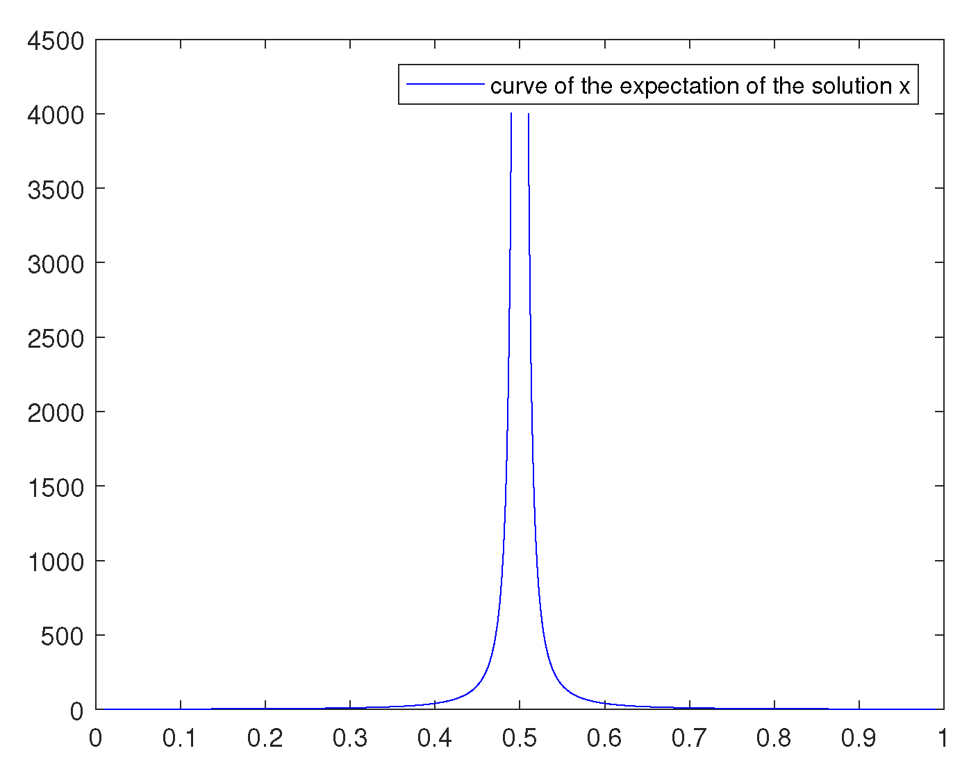
Example 2. Let , , , , and . Consider the following variational problem (
1)–(
2):
where with and and denote, respectively, the left and the right stochastic fractional Riemann–Liouville derivatives of order α. Resorting again to Theorem 1, we obtain the following stochastic fractional Euler–Lagrange differential equation:Following [7], we observe that and can be approximated as follows:andChoosing , we get the curve for as shown in Figure 1. One can increase the value of N under the condition one adds a sufficient number of initial values related to some degrees of derivatives of . This particular question is similar to the standard fractional calculus and we refer the interested reader to the book [7]. 6. Conclusions
Numerous works related to the calculus of variations, addressing different optimization problems by means of classical, stochastic, and fractional derivatives through appropriate Euler-Lagrange equations, exist in the literature. To extend available results to a stochastic-fractional framework, we have established in this work new definitions associated to left and right stochastic Riemann–Liouville/Caputo fractional integrals and derivatives, together with some properties of boundedness, linearity, additivity and interaction between involved operators. Furthermore, we have proven new integration by parts theorems, according to the novel definitions, which have a central role for the establishment of the stochastic Riemann–Liouville/Caputo fractional Euler–Lagrange equations. The obtained stochastic Riemann–Liouville/Caputo fractional Euler–Lagrange equations generalize those available on the literature of fractional calculus. Moreover, the results of the paper motivate readers and researchers to go on and further develop the theory now initiated.
It is important to note that the mathematical background used in the original fractional calculus differs from what we have established here for the stochastic fractional case. Additionally, the six constructed definitions for the left and right stochastic Riemann–Liouville/Caputo integral/derivative operators, as well as proved integration by parts formulas, differ totally to those available in the fractional calculus theory: the first are applied to second order stochastic processes, and the second act on deterministic absolute continuous functions. Furthermore, our stochastic fractional Euler–Lagrange equations serve as necessary optimality conditions to optimization problems subject to unknown stochastic processes that can be effectively approximated by numerical methods: such equations might be transformed to ones subject to unknown deterministic functions that are the expectation , for instance, when the random variables follow the assumption of normality, which is instructive to approximate its expectation via stochastic fractional Euler–Lagrange equations determined statistically by the hypothesis test in inferential statistics.
We claim that the new mathematical concepts we have introduced here are more natural than those already available in the literature, since it is intuitive and convenient to proceed via application of the expectation.


