Article

Comb Model with Non-Static Stochastic Resetting and Anomalous Diffusion

by
Maike Antonio Faustino dos Santos
1,2
1
Department of Physics, PUC-Rio, Rua Marquês de São Vicente, 225, Rio de Janeiro 22451-900, Brazil
2
National Institute of Science and Technology for Complex Systems, Rua Xavier Sigaud 150, Rio de Janeiro 22290-180, Brazil
Fractal Fract. 2020, 4(2), 28; https://doi.org/10.3390/fractalfract4020028
Submission received: 13 May 2020 / Revised: 16 June 2020 / Accepted: 17 June 2020 / Published: 22 June 2020
(This article belongs to the Special Issue The Craft of Fractional Modelling in Science and Engineering III)

Abstract

:
Nowadays, the stochastic resetting process is an attractive research topic in stochastic process. At the same time, a series of researches on stochastic diffusion in complex structures introduced ways to understand the anomalous diffusion in complex systems. In this work, we propose a non-static stochastic resetting model in the context of comb structure that consists of a structure formed by backbone in x axis and branches in y axis. Then, we find the exact analytical solutions for marginal distribution concerning x and y axis. Moreover, we show the time evolution behavior to mean square displacements (MSD) in both directions. As a consequence, the model revels that until the system reaches the equilibrium, i.e., constant MSD, there is a Brownian diffusion in y direction, i.e., ( Δ y ) 2 t , and a crossover between sub and ballistic diffusion behaviors in x direction, i.e., ( Δ x ) 2 t 1 2 and ( Δ x ) 2 t 2 respectively. For static stochastic resetting, the ballistic regime vanishes. Also, we consider the idealized model according to the memory kernels to investigate the exponential and tempered power-law memory kernels effects on diffusive behaviors. In this way, we expose a rich class of anomalous diffusion process with crossovers among them. The proposal and the techniques applied in this work are useful to describe random walkers with non-static stochastic resetting on comb structure.

1. Introduction

The statistical models in physics offer ways to understand the implicit behaviors of the stochastic process in nature. Therefore to find suitable tools and models to describe them is crucial to advance the understatement of a natural and artificial stochastic process. Currently, the stochastic resetting process have attracted the attention of many researchers. This kind of process admits that the systems return to initial condition after a time chosen randomly, so the system starts the random process again and again. Thereby, the stochastic resetting models have found applications in backtrack recovery by RNA polymerases [1], non-equilibrium physics [2], first passage under stochastic resetting [3,4], and others [5,6]. In this context, the stochastic resetting to random walks was proposed through a diffusion model [7] by M. R. Evans and S. N. Majumdar. This model [7] has been investigated in contexts as optimization of search process [8,9], coagulation process [10], anomalous diffusion process [11,12], fractional calculus to include Lévy flights in stochastic resetting model [13]. The works [12,14] use new fractional-time derivatives in stochastic resetting models to do a unified approach with anomalous diffusion process. Furthermore, the diffusion equation with stochastic resetting can also be interpreted in terms of exponential memory kernel [15].
The main feature of usual diffusion (or free Brownian diffusion) is a linear evolution of time to the mean square displacement, i.e., ( x x ) 2 t . Nevertheless, the class of phenomena which is not described by the usual diffusion is commonly known as anomalous diffusion (or fractional diffusion), and can be classified by power-law function like ( x x ) 2 t α , in which ( ) = R ( ) f ( x , t ) d x ( f ( x , t ) is a distribution function). To 0 < α < 1 the system is sub-diffusive, to 1 < α < 2 occurs the super-diffusion. In particular cases, to α = 2 the diffusion is ballistic and for 2 < α occurs the hyper diffusive process. These type of diffusion typically is approached through the fractional calculus that deforms a differential operator in diffusion equation that becomes a generalized diffusion process [16,17,18,19,20,21,22]. Here, it is important make clear that anomalous diffusion phenomena go beyond of these formalisms and appears as a natural consequence in many statistical physics problems to theoretical and experimental contexts associate to different mechanisms [23,24].
In this broad scenario of the anomalous diffusion in complex structures, the greatest advances came in the 1980s, when fractal geometry was introduced by B. B. Mandelbrot [25,26], and has been extensively investigated in the most diverse situations in nature. In a fractal, the diffusion in general is anomalous since the fractal dimension d w is linked to the mean square value as follows: x 2 t α with α = 2 d W . When d w = 2 we have euclidean space, which implies the usual diffusion. Based on fractal geometry, Gefen et al. [27] demonstrated theoretically the occurrence of anomalous diffusion in percolation clusters in critically (that is, at the transition threshold). This result was confirmed through numerical simulation, which was based on the Monte-Carlo method and the random walk by Daniel ben-Avraham and Shlomo Havlin (1982) [28], H. Panday and Dietrich Stauffer (1983) [29]. In this direction, White and Barma’s model [30] is based on the random walk in a linear chain (backbone) of uniformly spaced sites. From each backbone site, there are finite linear chain (a branch) of sites. These branches occur in the direction of the field and their length is given at random employing the probability distribution. Due to the resemblance to a comb, the backbone corresponds to the stem and branches. This structure was called random comb, comb-like structure or comb model. A continuous description of the random walk for the comb model was proposed in 1991, by Arkhincheev and Baskin, in the article entitled Anomalous diffusion and drift in a comb model of percolation clusters [31]. The main idea is to modify the two-dimensional diffusion equation as follows
t f ( x , y , t ) = δ ( y ) K x 2 x 2 f ( x , y , t ) + K y 2 y 2 f ( x , y , t ) ,
K y and K x being the diffusion coefficients in the directions x and y. The Equation (1) gives us the following quadratic deviations y 2 t and x 2 t 1 2 , which is anomalous in x direction. The diffusion in the direction is anomalous, demonstrating that the geometric restrictions in the system naturally imply anomalous behavior for the diffusion. In addition to elucidating some concepts about diffusion and revealing connections with clusters and fractals, the comb model can be used to describe the dynamics of ions in neuron dendrites [32]. Indeed the comb structure has been the scene of many important problems in statistical physics. Recently, a series of investigations have been carried out using several diffusive models on comb structure, we can mention some of these advances: models associated with sub-diffusive processes on fractal comb [33], heterogeneous diffusion models on comb structure [34], first passage problem associated with systems that remove particles on the structure of the comb [35], a random search for target [36] and fractional kinetic on comb structure [37]. In this sense, this work brings a detailed study about non-static stochastic resetting [12] on comb structure. In the following, we analyze the anomalous diffusion crossovers caused by memory effects.
Inspired on diffusion in complex structures models, this work proposes a diffusion model suitable to approach the stochastic resetting process phenomena on comb structure. In Section 2, we propose the model and explain the main aspects of the comb structure, finding the exact solution and their stationary limits. Moreover, we achieve the MSD behavior to short times which present sub-diffusive process in x direction and usual diffusive process in y direction. In Section 3, we consider the model proposed by us under the point of view of the memory kernels in diffusive terms. In this sense, we present the analytical expressions to ( x x ) 2 and ( y y ) 2 averages that revel a rich class of anomalous diffusion behaviors which include crossovers among them. Finally, in Section 4, we draw conclusions and outline some perspectives.

2. The Model

The comb model was initially introduced to investigate anomalous diffusion in percolation clusters according to [30]. Considering our perspective, here we examine the comb model (Equation (1)) with an additional term that represents the stochastic resetting process as follows
t f ( x , y , t ) = δ ( y ) K x 2 x 2 f ( x , y , t ) + K y 2 y 2 f ( x , y , t ) + R ( x , y , t ) ,
in which R ( x , y , t ) consist in a bi-dimensional version of a recent purpose of non-static stochastic resetting [12] which is write as follows
R ( x , y , t ) = κ f ( x , y , t ) + κ δ ( y ) δ ( x v t ) ,
in which the static case occurs to v = 0 [7] we recovered one of particular cases approached by A. A. Tateishi in Ref. [38]. Moreover we have the boundary conditions and initial condition defined by
f ( ± , y , t ) = f ( x , ± , t ) = 0 a n d f ( x , y , 0 ) = δ ( x ) δ ( y ) .
The K y and K x in Equation (2) are diffusion coefficients in the x and y directions. The presence of the Dirac delta in Equation (2) implies that the diffusion in the x-direction only occurs when y = 0 , see the walker represented by a black point on x-axis in Figure 1a. Consequently, the diffusion in the y-direction always occurs perpendicularly to the x-axis, see the black point out of the x-axis in Figure 1a. Term (3) in Equation (2) permits the occurrence of the stochastic resetting on a non-static position, so the term κ f ( x , y , t ) remove randomly the walker in a system with a rate κ and the term κ δ ( y ) δ ( x v t ) relocate the removed walkers in position ( y = 0 , x = v t ) , see the red point in Figure 1b which represents a walker that is relocated in the black point that moves on time with v velocity.
Now, to find the solution to Equation (2) with condition (4) we consider the F { g ( x ) } = g ( x ) e i k x x d x and g ˜ ( s ) = L { g ( t ) } = 0 g ( t ) e s t d t that are the Fourier and Laplace transforms, respectively. Assuming the Fourier transforms on x , y and a Laplace transform on time t, we obtain
F y { F x { f ˜ ( x , y , s ) } } = 1 + κ s + i v k x K x k x 2 F x { f ˜ ( k x , y = 0 , s ) } s + κ + K y k y 2 .
Realizing the inverse Fourier transform under k y variable we obtain
F x { f ˜ ( x , y , s ) } = 1 + κ s + i v k x exp s + κ K y | y | 2 K y ( s + κ ) K y k x 2 F x { f ˜ ( x , y = 0 , s ) } exp s + κ K y | y | 2 K y ( s + κ ) .
Considering y = 0 in Equation (6), we obtain the exact solution to F x { f ˜ ( k x , y = 0 , s ) } as
F x { f ˜ ( x , y = 0 , s ) } = 1 + κ s + i v k x 2 K y ( s + κ ) + K x k x 2 ,
that permits to rewrite the Equation (5) as follows
F y { F x { f ˜ ( x , y , s ) } } = 2 K y ( s + κ ) 2 K y ( s + κ ) + K x k x 2 1 + κ s + i v k x s + κ + K y k y 2 .
To simplify our analysis, we consider the marginal distribution functions as did in Ref. [39], which imply the definitions
f ˜ 1 ( x , s ) = f ˜ ( x , y , s ) d y = F y { f ˜ ( x , y , s ) } | k y = 0
and
f ˜ 2 ( y , s ) = f ˜ ( x , y , s ) d x = F x { f ˜ ( x , y , s ) } | k x = 0 .
Using the marginal distribution functions (Equations (9) and (10)) and solution in Fourier–Laplace transform in Equation (8), we obtain
F x { f ˜ 1 ( x , s ) } = 1 + κ s + i v k x 2 K y ( s + κ ) 1 2 2 K y ( s + κ ) + K x k x 2 ,
and
F y { f ˜ 2 ( y , s ) } = 1 s s + κ s + κ + K y k y 2 .
Here, we need realize inverse transformations to show the exact solutions to marginal distributions in terms of the x , y , t coordinates. Let us solve the inverse Laplace transform of the Equation (11) by use the Prudnikov table [40] that possibility the inversion of a general function L 1 { F ( 2 s ) } opening a way to find the exact solution to marginal distribution F x { f 1 ( x , t ) } as follows
F x { f 1 ( x , t ) } = t 3 2 π 0 e u 2 t κ t g ¯ ( k x , u ) d u + 0 t t 3 2 π 0 e u 2 t κ t g ¯ ( k x , u ) exp [ i v k x ( t t ) ] d u d t ,
in which
g ¯ ( k x , t ) = 4 e κ t K y 1 K x k x 2 e K x t k x 2 K y K x k x 2 .
Then, by realizing the inverse Fourier transforms of function F x { f ˜ 1 ( x , s ) } , i.e., (13), we obtain
f 1 ( x , t ) = t 3 2 π 0 e u 2 t κ t g ( x , u ) d u + 0 t t 3 2 π 0 e u 2 t κ t g ( x v ( t t ) , u ) d u d t ,
in which
g ( x , t ) = 4 t K y K x π exp K y x 2 4 K x t 2 K y K x x erfc K y 2 t K x | x | 2 .
That for static stochastic resetting case, i.e., v = 0 , we obtain the follow particular solution
f 1 ( x , t ) = t 3 2 π 0 e u 2 t κ t g ( x , u ) d u + 0 t 0 t 3 2 π e u 2 t κ t g ( x , u ) d u d t ,
that applying the Tauberian theorem, i.e., lim t g ( t ) = lim s 0 L { g ( s ) } in Laplace transform of Equation (17), that implies stationary solution
f e s t 1 ( x ) = K y κ 2 K x exp 2 K y κ K x | x | .
This stationary solution revels that marginal distribution in x-axis is influenced by dynamical proprieties of y-axis.
The inverse transform of the Equation (13) in Fourier and Laplace space is written as follows
f 2 ( y , t ) = L 1 s + κ 2 s K y exp s + κ K y | y | = e κ t e y 2 4 K y t 2 K y π t + κ 0 t e κ t e y 2 4 K y t 2 K y π t d t .
that for a long time implies stationary marginal distribution
f e s t 2 ( y ) = κ 4 K y exp κ K y | y | .
The stationary solution in y-axis coincides with Evans–Majumdar result [7] to uni-dimensional problem. The marginal solutions (15) and (19) make it clear that stochastic resetting affects only the marginal distribution in x-axis.
The time evolution of distributions associate to static restart point ( v = 0 ), i.e., Equations (17) and (19), are presented in Figure 2. Moreover, Figure 2a,b contains dotted curves that represent the stationary solutions (18) and (20), it shows that system could find the equilibrium to t = 10 when K ( x , y ) = 1 and κ = 1 . Figure 3 shows the distribution shape in relation to x v t , that for high valuer of time the distribution shapes converge to red one. The non-static stochastic resetting was explored to fractional diffusion in one dimension case in Ref. [12].
The mean square displacement (MSD) can elucidate the diffusion types to short time valuers. Here, we have ( x x ) 2 = x 2 x 2 , the same to ( y y ) 2 = y 2 y 2 = y 2 ( y = 0 ). In this sense, we can define generalized natural moments x n and y n through the marginal distributions as follow
x n = i n L 1 lim k x 0 n k x n F x { f 1 ( x , s ) } ,
y n = i n L 1 lim k y 0 n k y n F y { f 2 ( y , s ) } .
Using the Equations (15) and (19) and Equations (21) and (22) we obtain
( x x ) 2 = K x K y κ Erf [ κ t ] + 2 v 2 e κ t ( sinh [ κ t ] κ t ) κ 2 ,
( y y ) 2 = 2 K y κ 1 e κ t .
For long time valuers we have the asymptotic limits ( Δ x ) 2 v 2 κ 2 + K x / κ K y and ( Δ y ) 2 2 K y / κ . For short time ( t 1 / κ ) the diffusion in relation to the y direction obeys the usual behavior, i.e., ( Δ y ) 2 2 K y t , and to x direction we has ( Δ x ) 2 2 K x t 1 2 / π K y . All this asymptotic behaviors are exemplified in Figure 4a,b for static case, i.e., v = 0 . The non-static case was presented in Figure 5, which presents a crossover between sub and ballistic diffusive regimes before the system reaches the equilibrium. The ballistic regime is exclusively due non-stochastic resetting process before the system comes out of inertial state.
A parallel research was made by V. Domazetoski et al. in Ref. [41]. The authors consider the stochastic resetting problem in 3-dimensional comb-like structure. In fact, the marginal distributions in Laplace space to particular of static resetting case ( v = 0 ), i.e., Laplace transform of Equations (17) and (19) correspond to marginal distribution in Laplace space found by V. Domazetoski et al. in Equations (40) and (41) in Ref. [41]. Then, the first part of our results coincide only in this specific point with their respective MSD, which is a clear signal of a very effervescent research line. Moreover, in the next section, we consider memory kernels in Laplacian terms with kernels that are connected with a Cattaneo process types.

3. The Model with Memory Kernels Effects: Crossover between Anomalous Diffusion Regimes

The memory effects in diffusion process have been investigated in many current problems [14,17,18,19,42]. This memory kernel techniques have been a suitable tool to introduce anomalous diffusion in transport models. In this sense, here we rewrite the model (2) with general convolution kernels on diffusive terms K x ( t ) and K y ( t ) as follows
t f ( x , y , t ) = δ ( y ) 0 t K x ( t t ) 2 x 2 f ( x , y , t ) d t + 0 t K y ( t t ) 2 y 2 f ( x , y , t ) d t κ f ( x , y , t ) + δ ( y ) δ ( x v t ) ,
in which boundaries and initial conditions were presented in relations (4). Realizing the Laplace transform on time t and Fourier transforms on x , y in Equation (25), we obtain
F y { F x { f ˜ ( x , y , s ) } } = 1 + κ s + i v k x K ˜ x ( s ) k x 2 F x { f ˜ ( k x , y = 0 , s ) } s + κ + K ˜ y ( s ) k y 2 ,
that has the same mathematical structure of Equation (5). Then, as in previous calculus we obtain the follow solution in Laplace-Fourier space
F y { F x { f ˜ ( x , y , s ) } } = 2 K ˜ y ( s ) ( s + κ ) 2 K ˜ y ( s ) ( s + κ ) + K ˜ x ( s ) k x 2 1 + κ s + i v k x s + κ + K ˜ y ( s ) k y 2 .
Thereby, using this general relations in Equations (21) and (22) we obtain the follow equations
( x x ) 2 = L 1 K ˜ x ( s ) s K ˜ y ( s ) ( κ + s ) + 2 κ v 2 s 3 ( κ + s ) L 1 κ v s 2 ( κ + s ) 2
( y y ) 2 = L 1 2 K ˜ y ( s ) s ( s + κ ) .
Now, we consider two cases to analyze the memory effects in non-static stochastic resetting on comb structure. To assure the non-negativity of marginal distributions (safe ones) [43] we consider a kernel class that implies two marginal solutions in Laplace space that can be identified with non-negative uni-dimensional solution of generalized diffusion equations. The first one is an exponential memory kernel that connects the marginal solutions in Laplace space to well known uni-dimensional Cattaneo diffusion equation [44] or finite velocity effect on comb structure [37,39]. The second one is a tempered power-law kernel that connects the marginal solutions in Laplace space to uni-dimensional Prabhakar-tempered diffusion equation [45] to specific choices of the fractional index. Then, to consider other kernel classes the conditions investigated by I. M. Sokolov in Ref. [43] need be verified to avoid the negative solutions.

3.1. First Case: Exponential Memory in Diffusion Terms

The exponential kernels in convolution term of diffusion equation implies a memory effects associate to Cattaneo equation, see Ref. [44,46] for more details. Therefore, we write the kernels as follows
K x ( t ) = K x e t τ τ and K y ( t ) = K y e t τ τ .
The inverse Laplace transforms of Equations (28) and (29) combined with memory kernels (30) imply
( x x ) 2 = K x t τ K y e 1 2 t κ + 1 τ I 0 1 2 t κ 1 τ + I 1 1 2 t κ 1 τ + 0 t K x t τ τ K y e 1 2 t κ + 1 τ I 0 1 2 t κ 1 τ + I 1 1 2 t κ 1 τ d t + 2 v 2 e κ t ( sinh [ κ t ] κ t ) κ 2 ,
and
( y y ) 2 = 2 K y 1 κ τ e t τ κ τ 1 + e κ t κ ( κ τ 1 ) ,
in which I 0 [ z ] is a modified Bessel functions. To short time, we obtain the usual behavior in x-direction, i.e., ( x x ) 2 t , and the ballistic behavior in y-direction, i.e., ( y y ) 2 t 2 . Figure 6 presents the MSD behavior on time to different τ valuers in exponential memory kernels with v = 0 . Thereby, Figure 6a,b to small τ valuers and t 1 presents the sub-diffusive ( ( x x ) 2 t 1 2 ) and usual diffusive regimes ( ( y y ) 2 t ), respectively. The non-static case ( v 0 ) in MSD appears on x-axis in Figure 7 that displays three diffusive regimes before the system reaches the stationary state from MSD point of view, more specifically the MSD in x-axis present ballistic, usual and hyper diffusive regimes to t < 1 / κ .

3.2. Second Case: Tempered Power-Law Memory in Diffusion Terms

The second case consider a mix of power-law kernels with exponential factor. This operator types is well known in the literature by tempered memory kernels, a remarkable feature is the truncation in power-law functions [47]. Thereby, we can write they as follow
K x ( t ) = K x t α Γ [ 1 α ] e t τ τ
K y ( t ) = K y t β Γ [ 1 β ] e t τ τ ,
in which 0 < α 1 and 0 < β 1 . The tempered kernels involve a mix of two or more functions to approach generalization of the fractional stable statistics [48]. Then, the “tempered” kernel types allow suitable truncation effects which imply crossover process among diffusive process [45,49,50]. The tempered kernels ((33) and (34)) in Equations (28) and (29) imply the follow inverse expressions
( x x ) 2 = K x τ K y κ 0 t erf κ ( t t ) e t τ t β 1 2 α Γ 1 α + β 1 2 d t + 2 v 2 e κ t ( sinh [ κ t ] κ t ) κ 2 ,
and
( y y ) 2 = 2 K y 0 t 1 κ τ e κ t t κ τ t β e t τ Γ [ 1 β ] d t .
These MSD revel that for short time ( t τ ) we have ( x x ) 2 t 3 2 α + 1 2 ( β 1 ) and ( y y ) 2 t 2 β as presented in Figure 8a,b, respectively. These figures present a wide class of diffusion types to static resetting case and different α , β parameters. Moreover, to times of order t 1 and small τ valuer, Figure 8 shows to intermediate diffusive regimes ( x x ) 2 t 1 2 and ( y y ) 2 t 
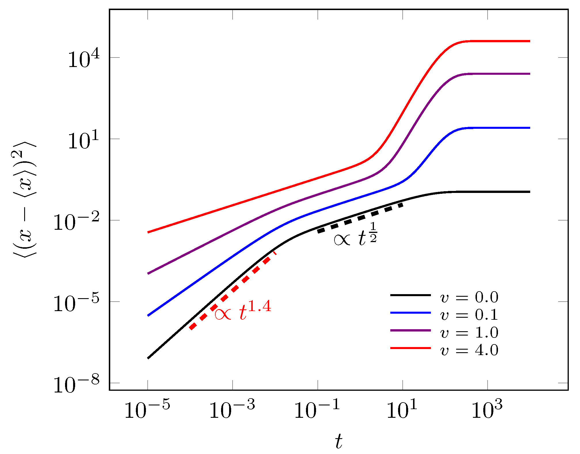
that correspond to regimes out of power-law memory influence. The non-static stochastic resetting effects appear in Figure 9 to different velocity valuers. This figure makes clear that the there are a crossover of two super-diffusive process with a sub-diffusive process among them before the plateau state. Here, we can comment on non-truncation effect in power-law memory kernels ((33) and (34)). To this case, there is no exponential truncation function which implies vanishing of the intermediate behaviors ( Δ x ) 2 t 1 2 , ( Δ y ) 2 t and ( Δ x ) 2 t 1 2 in Figure 8a,b and Figure 9 respectively. Therefore, the exponential truncation is responsible to the vanishing of the power-law function effects ( t > τ ) resulting the crossover in MSD with a intermediate time regimes associated to the usual-diffusion on comb structure reported in Equations (23) and (24) before the system reaches the plateau state.
Other kernel classes can be considered in general model (25) that can imply new annealed disorder mechanisms [38]. Particularly considering K y ( t ) = δ ( t ) K y in model (25) we obtain a diffusion model that for non-stochastic resetting case, i.e., κ = 0 , we obtain a particular case of comb model with slow and ultraslow diffusion investigate by T. Sandev et al. in Ref. [51].

4. Conclusions

Daily, the stochastic process has introduced a vast quantity of new techniques and applications in nature. In this work, we investigated the non-static stochastic resetting process on comb model. The non-static characteristic allows resetting the system on a point that moves with a constant velocity v on dorsal backbone in comb structure. We presented the exact analytical solution to marginal distributions to x and y axis. Moreover, the results show that MSD behavior to x direction initially has a sub-diffusive regime ( x x ) 2 t 1 2 followed by a ballistic regime due non-static feature, after that the systems reaches the stationary regime to MSD. In y direction the result revels that non-static characteristic has not influence, so we find a Brownian behavior to a short time, i.e., ( y y ) 2 t and a constant MSD for long time. Finally, we considered memory kernels in diffusion terms of the model to investigate the diffusive process in different directions on comb structure. To the first memory case, we considered exponential memory kernel, that implies MSD for short times ( t < τ ) as ( x x ) 2 t and ( y y ) 2 t 2 in x and y directions, respectively. Its results differ from the usual case due to the presence of the exponential kernels effects associated with Cattaneo equation type. In the second memory case, we considered a tempered power-law memory kernel that imply anomalous diffusion process to very short times ( t < τ ), that imply ( x x ) 2 t 3 2 α + 1 2 ( β 1 ) and ( y y ) 2 t 2 β to x and y directions, respectively. After this time regime, the system goes to a time regime ( τ < t 1 / κ ) governed by a sub or usual diffusion process. Then, for times of order t 1 / κ there is a third regime that presents super or hyper diffusion process to non-static stochastic resetting case v 0 . These results implied a robust variety of anomalous diffusion process. In fact, both memory kernels considered admit a crossover between two or more anomalous diffusion process before the system reaches the stationary state to MSD point of view.
The diffusion models introduced in this work allow to describe the transport process on comb structure with non-static stochastic resetting and memory effects. Thereby, this work opens possibilities to investigate the stochastic resetting problem for mesh and fractal grids considering different memory function associated with Mittag–Leffler functions.

Funding

This research received no external funding.

Acknowledgments

Maike Antonio Faustino dos Santos acknowledges the support of the Brazilian agency CAPES, Pontifical Catholic University of Rio de Janeiro and National Institute of Science and Technology for Complex Systems (INCT-SC). Moreover, Maike Antonio Faustino dos Santos would like to thank all referees of this work for their important appointments, suggestions and their careful reading.

Conflicts of Interest

The author declares no conflict of interest.

References

  1. Roldán, É.; Lisica, A.; Sánchez-Taltavull, D.; Grill, S.W. Stochastic resetting in backtrack recovery by RNA polymerases. Phys. Rev. E 2016, 93, 062411. [Google Scholar] [CrossRef] [PubMed] [Green Version]
  2. Eule, S.; Metzger, J.J. Non-equilibrium steady states of stochastic processes with intermittent resetting. New J. Phys. 2016, 18, 033006. [Google Scholar] [CrossRef]
  3. Campos, D.; Méndez, V. Phase transitions in optimal search times: How random walkers should combine resetting and flight scales. Phys. Rev. E 2015, 92, 062115. [Google Scholar] [CrossRef] [PubMed] [Green Version]
  4. Pal, A.; Prasad, V.V. First passage under stochastic resetting in an interval. Phys. Rev. E 2019, 99, 032123. [Google Scholar] [CrossRef] [Green Version]
  5. Fuchs, J.; Goldt, S.; Seifert, U. Stochastic thermodynamics of resetting. EPL 2016, 113, 60009. [Google Scholar] [CrossRef] [Green Version]
  6. Evans, M.R.; Majumdar, S.N.; Schehr, G. Stochastic resetting and applications. J. Phys. A 2020, 53, 193001. [Google Scholar] [CrossRef]
  7. Evans, M.R.; Majumdar, S.N. Diffusion with stochastic resetting. Phys. Rev. Lett. 2011, 106, 160601. [Google Scholar] [CrossRef] [Green Version]
  8. Chechkin, A.; Sokolov, I.M. Random search with resetting: A unified renewal approach. Phys. Rev. Lett. 2018, 121, 050601. [Google Scholar] [CrossRef]
  9. Mejía-Monasterio, C.; Oshanin, G.; Schehr, G. First passages for a search by a swarm of independent random searchers. J. Stat. Mech. Theory Exp. 2011, 2011, P06022. [Google Scholar] [CrossRef] [Green Version]
  10. Durang, X.; Henkel, M.; Park, H. The statistical mechanics of the coagulation–diffusion process with a stochastic reset. J. Phys. A 2014, 47, 045002. [Google Scholar] [CrossRef] [Green Version]
  11. Masoliver, J.; Montero, M. Anomalous diffusion under stochastic resettings: A general approach. Phys. Rev. E 2019, 100, 042103. [Google Scholar] [CrossRef] [PubMed]
  12. Dos Santos, M.A.F. Fractional prabhakar derivative in diffusion equation with non-static stochastic resetting. Physics 2019, 1, 5. [Google Scholar] [CrossRef] [Green Version]
  13. Kuśmierz, Ł.; Gudowska-Nowak, E. Optimal first-arrival times in Lévy flights with resetting. Phys. Rev. E 2015, 92, 052127. [Google Scholar]
  14. Dos Santos, M.A.F. Non-Gaussian distributions to random walk in the context of memory kernels. Fractal Fract. 2018, 2, 20. [Google Scholar] [CrossRef] [Green Version]
  15. Tateishi, A.A.; Ribeiro, H.V.; Lenzi, E.K. The role of fractional time-derivative operators on anomalous diffusion. Front. Phys. 2017, 5, 52. [Google Scholar] [CrossRef] [Green Version]
  16. Barkai, E. Fractional Fokker-Planck equation, solution, and application. Phys. Rev. E 2001, 63, 046118. [Google Scholar] [CrossRef] [Green Version]
  17. Dos Santos, M.A.F. Analytic approaches of the anomalous diffusion: A review. Chaos Solitons Fractals 2019, 124, 86–96. [Google Scholar] [CrossRef] [Green Version]
  18. Hristov, J. Diffusion models of heat and momentum with weakly singular kernels in the fading memories: How the integral-balance method can be applied? Therm. Sci. 2015, 19, 947–957. [Google Scholar] [CrossRef]
  19. Hristov, J. On the Atangana–Baleanu derivative and its relation to the fading memory concept: The diffusion equation formulation. In Fractional Derivatives with Mittag–Leffler Kernel; Springer International Publishing: Cham, Switzerland, 2019; pp. 175–193. [Google Scholar]
  20. Sene, N. Analytical solutions and numerical schemes of certain generalized fractional diffusion models. Eur. Phys. J. Plus 2019, 134, 199. [Google Scholar] [CrossRef]
  21. Sene, N. Analytical solutions of Hristov diffusion equations with non-singular fractional derivatives. Chaos Interdiscip. J. Nonlinear Sci. 2019, 29, 023112. [Google Scholar] [CrossRef]
  22. Dos Santos, M.A.F. Mittag–leffler memory kernel in lévy flights. Mathematics 2019, 7, 766. [Google Scholar] [CrossRef] [Green Version]
  23. Bouchaud, J.P.; Georges, A. Anomalous diffusion in disordered media: Statistical mechanisms, models and physical applications. Phys. Rep. 1990, 195, 127–293. [Google Scholar] [CrossRef]
  24. Oliveira, F.A.; Ferreira, R.; Lapas, L.C.; Vainstein, M.H. Anomalous diffusion: A basic mechanism for the evolution of inhomogeneous systems. Front. Phys. 2019, 7, 18. [Google Scholar] [CrossRef] [Green Version]
  25. Mandelbrot, B.B. The Fractal Geometry of Nature; WH Freeman New York: New York, NY, USA, 1983; Volume 173. [Google Scholar]
  26. Mandelbrot, B.B. Fractals: Form, Chance and Dimension; Mandelbrot, B.B., Ed.; WH Freeman & Co.: San Francisco, CA, USA, 1979; 365p. [Google Scholar]
  27. Gefen, Y.; Aharony, A.; Alexander, S. Anomalous diffusion on percolating clusters. Phys. Rev. Lett. 1983, 50, 77. [Google Scholar] [CrossRef]
  28. Ben-Avraham, D.; Havlin, S. Diffusion on percolation clusters at criticality. J. Phys. A 1982, 15, L691. [Google Scholar] [CrossRef] [Green Version]
  29. Pandey, R.; Stauffer, D. Confirmation of dynamical scaling at the percolation threshold. Phys. Rev. Lett. 1983, 51, 527. [Google Scholar] [CrossRef]
  30. White, S.R.; Barma, M. Field-induced drift and trapping in percolation networks. J. Phys. A 1984, 17, 2995. [Google Scholar] [CrossRef]
  31. Arkhincheev, V.; Baskin, E. Anomalous diffusion and drift in a comb model of percolation clusters. Sov. Phys. JETP 1991, 73, 161–300. [Google Scholar]
  32. Méndez, V.; Iomin, A. Comb-like models for transport along spiny dendrites. Chaos Solitons Fractals 2013, 53, 46–51. [Google Scholar] [CrossRef] [Green Version]
  33. Iomin, A. Subdiffusion on a fractal comb. Phys. Rev. E 2011, 83, 052106. [Google Scholar] [CrossRef] [Green Version]
  34. Sandev, T.; Schulz, A.; Kantz, H.; Iomin, A. Heterogeneous diffusion in comb and fractal grid structures. Chaos Solitons Fractals 2018, 114, 551–555. [Google Scholar] [CrossRef] [Green Version]
  35. Tateishi, A.A.; Michels, F.S.; Dos Santos, M.A.F.; Lenzi, E.K.; Ribeiro, H.V. First passage time for a diffusive process under a geometric constraint. J. Stat. Mech. Theory Exp. 2013, 2013, P09017. [Google Scholar] [CrossRef]
  36. Sandev, T.; Iomin, A.; Kocarev, L. Random search on comb. J. Phys. A 2019, 52, 465001. [Google Scholar] [CrossRef]
  37. Liu, L.; Zheng, L.; Zhang, X. Fractional anomalous diffusion with Cattaneo–Christov flux effects in a comb-like structure. Appl. Math. Model. 2016, 40, 6663–6675. [Google Scholar] [CrossRef]
  38. Tateishi, A.A.; Ribeiro, H.V.; Sandev, T.; Petreska, I.; Lenzi, E.K. Quenched and annealed disorder mechanisms in comb models with fractional operators. Phys. Rev. E 2020, 101, 022135. [Google Scholar] [CrossRef] [Green Version]
  39. Sandev, T.; Iomin, A. Finite-velocity diffusion on a comb. EPL 2018, 124, 20005. [Google Scholar] [CrossRef] [Green Version]
  40. Prudnikov, A.; Brychkov, Y.A.; Marichev, O.I. Integrals and Series, Volume 4, Direct Laplace Transforms; Gordon and Breach: New York, NY, USA, 1992; Volume 4. [Google Scholar]
  41. Domazetoski, V.; Masó-Puigdellosas, A.; Sandev, T.; Méndez, V.; Iomin, A.; Kocarev, L. Stochastic resetting on comb-like structures. arXiv 2020, arXiv:2005.11575. [Google Scholar]
  42. Dos Santos, M.A.F. From continuous-time random walks to controlled-diffusion reaction. J. Stat. Mech. Theory Exp. 2019, 2019, 033214. [Google Scholar] [CrossRef] [Green Version]
  43. Sokolov, I.M. Solutions of a class of non-Markovian Fokker-Planck equations. Phys. Rev. E 2002, 66, 041101. [Google Scholar] [CrossRef] [Green Version]
  44. Compte, A.; Metzler, R. The generalized Cattaneo equation for the description of anomalous transport processes. J. Phys. A 1997, 30, 7277. [Google Scholar] [CrossRef]
  45. Sandev, T.; Deng, W.; Xu, P. Models for characterizing the transition among anomalous diffusions with different diffusion exponents. J. Phys. A 2018, 51, 405002. [Google Scholar] [CrossRef] [Green Version]
  46. Liu, L.; Zheng, L.; Fan, Y.; Chen, Y.; Liu, F. Comb model for the anomalous diffusion with dual-phase-lag constitutive relation. Commun. Nonlinear Sci. Numer. Simul. 2018, 63, 135–144. [Google Scholar] [CrossRef] [Green Version]
  47. Liemert, A.; Sandev, T.; Kantz, H. Generalized Langevin equation with tempered memory kernel. Physica A 2017, 466, 356–369. [Google Scholar] [CrossRef]
  48. Rosiński, J. Tempering stable processes. Stoch. Process. Their Appl. 2007, 117, 677–707. [Google Scholar] [CrossRef] [Green Version]
  49. Koponen, I. Analytic approach to the problem of convergence of truncated Lévy flights towards the Gaussian stochastic process. Phys. Rev. E 1995, 52, 1197. [Google Scholar] [CrossRef]
  50. Sibatov, R.T.; Sun, H.G. Tempered fractional equations for quantum transport in mesoscopic one-dimensional systems with fractal disorder. Fractal Fract. 2019, 3, 47. [Google Scholar] [CrossRef] [Green Version]
  51. Sandev, T.; Iomin, A.; Kantz, H.; Metzler, R.; Chechkin, A. Comb model with slow and ultraslow diffusion. Math. Model. Nat. Phenom. 2016, 11, 18–33. [Google Scholar] [CrossRef]
Figure 1. The different situation to walkers that moves on comb structure. Figure (a) shows two walkers, one on x-axis ( y = 0 ) that admits the next step in both directions, the other walker out of the x a x i s ( y 0 ) can move only in y-axis to anyone y 0 . Figure (b) shows only one walker on comb structure that is resetting to position x resetting = v t on black point.
Fractalfract 04 00028 g001
Figure 2. These figures represents time evolution behavior to marginal distributions to static stochastic resetting v = 0 . Figure (a) represents the solution (17) and Figure (b) represents the solution (19) to different time valuer. Both figures consider the parameter valuers as follow K x = K y = 1 and κ = 1 .
Fractalfract 04 00028 g002
Figure 3. This figure represents time evolution behavior to marginal distribution in x-axis (Equation (15) to non-static stochastic resetting. In this figure, we consider the parameter valuers as follow K x = K y = 1 , v = 1 and κ = 1 .
Fractalfract 04 00028 g003
Figure 4. These figures represent time evolution of MSD behaviors in Equations (23) and (24) to static stochastic resetting case, i.e., v = 0 . Figure (a) represents the MSD on x-axis and Figure (b) represents the MSD on y-axis. Both figures consider the parameter valuers as follow K x = 1 and K y = 1 .
Fractalfract 04 00028 g004
Figure 5. This figure represents time evolution of MSD behavior x axis (Equations (23) and (24)) to non-static stochastic resetting case. In this figure we consider the parameter valuers as follow K x = 1 , K y = 1 , κ = 0.01 and different velocities to resetting point.
Fractalfract 04 00028 g005
Figure 6. These figures represent time evolution to MSD behaviors to static stochastic resetting, i.e., v = 0 . Figure (a) represents the MSD associated to Equation (31) and Figure (b) represents the MSD associated to Equation (32) to different τ valuers. Both figures consider the parameter valuers as follows K x = K y = 1 and κ = 0.02 .
Fractalfract 04 00028 g006aFractalfract 04 00028 g006b
Figure 7. This figure represents time evolution of MSD behavior x axis (Equation (31)) to non-static stochastic resetting case. In this figure, we consider the parameter valuers as follow K x = 1 , K y = 1 , τ = 0.001 , κ = 0.02 and different velocities to resetting point.
Fractalfract 04 00028 g007
Figure 8. Figure (a) represents the MSD associated to Equation (35) for different α indexes with fixed β = 1 . Figure (b) represents the MSD associated to Equation (36) for different β valuers. Both figures consider the parameter valuers as follows K x = K y = 1 , κ = 0.02 and τ = 0.01 .
Fractalfract 04 00028 g008aFractalfract 04 00028 g008b
Figure 9. This figure represents time evolution of MSD behavior x axis (Equation (35)) to non-static stochastic resetting case, considering K x = 1 , K y = 1 , τ = 0.01 , κ = 0.02 , β = 1 , α = 0.1 and different velocities to resetting point.
Fractalfract 04 00028 g009

