1. Introduction and Model Formulation
The need to go beyond the Fourier heat conduction equation is experimentally proved under different conditions since decades. There are various situations where the classical Fourier constitutive law for heat conduction is not applicable (heat flux is not directly proportional to temperature gradient), such as heat conduction in heterogeneous materials or at low temperatures [
1,
2,
3].
Several generalizations of the Fourier heat conduction equation using integer-order derivatives are reviewed in [
4]. Among them is the Jeffreys-type heat conduction equation
where
T is the temperature,
and
are relaxation times,
is the thermal diffusivity,
denotes the position vector,
t is the temporal variable,
denotes the spatial Laplace operator. The Jeffreys-type Equation (
1) generalizes both the classical Fourier heat conduction equation, obtained by setting
in (
1) and the Cattaneo (or telegrapher’s) equation, obtained by setting
in (
1).
There are different constitutive relations, from where the Jeffreys-type partial differential Equation (
1) can be derived, with different interpretation of the coefficients. These are the first order differential Dual-Phase-Lag (DPL) constitutive model, introduced in [
5], which has the same form as the so called Jeffreys-type constitutive equation, introduced in [
4] in the context of rheology. Moreover, in one spatial dimension Equation (
1) can be derived from the Guyer–Krumhansl (GK) constitutive equation, which is related to the phenomenon of second sound in solids. For a concise overview of the above models we refer to the recent work [
6]. See also [
7] for a study of thermodynamical consistency of the aforementioned constitutive equations in one spatial dimension.
The Jeffreys-type heat transport Equation (
1) is studied analytically and numerically in different settings. One of its applications is as a model for thermal behavior in complex non-homogeneous media, such as living tissues. For instance, in [
8,
9] it is used in models of skin biothermomechanics. In the majority of the works both regimes (
and
) are of interest; see e.g., [
8,
9,
10,
11]. Let us note that the value of
in Equation (
1) represents the intensity of diffuse behavior of heat conduction process, while the value of
indicates the intensity of wave-like behavior; see, e.g., [
9] for a discussion. In [
8,
9] model (
1) is compared to other bioheat transfer models. In [
10] thermal damage to laser irradiated tissue is analyzed on the basis of the model (
1). An initial-value problem for the three-dimensional Equation (
1) with a positive localized source of short duration is studied in [
12], where unphysical behavior of the solution with negative values is found for
. In [
11] an analytical solution is derived for the Guyer–Krumhansl equation considering boundary conditions from laser flash experiment. Analytical studies of GK type equations can be also found in [
13,
14]. In [
15] Equation (
1) is recast into a heat diffusion equation with a non-singular memory kernel, where the relaxation term is expressed through the Caputo-Fabrizio time-fractional derivative.
Various time-fractional generalizations of the integer-order non-Fourier heat conduction models are studied. Fractional telegrapher’s equation are considered, e.g., in [
16,
17,
18], while the works [
19,
20] are devoted to fractional Cattaneo-type equations of distributed order. In [
21] a number of time-fractional Cattaneo models are shown to produce the crossover of the mean squared displacement from superdiffusion to subdiffusion.
A time-fractional generalization of the Jeffreys-type heat conduction Equation (
1) is proposed in [
22]. According to the fractional Jeffreys-type constitutive law ([
22,
23] (Chapter 7)) the heat flux vector
and the temperature
T are related via the equation
where
is the heat flux vector,
and
are generalized relaxation times,
k is the thermal conductivity,
denotes the Riemann–Liouville fractional time-derivative of order
, and ∇ denotes the gradient operator, acting with respect to the space variables. Combining Equation (
2) with the energy balance equation
where
C denotes the heat capacity, one finds the following fractional Jeffreys-type heat conduction equation
where
is the thermal diffusivity. For notational simplicity we set in the present work
. We assume arbitrary initial temperature distribution,
and zero initial heat flux
The one-dimensional Cauchy problem for Equation (
4) is solved analytically in ([
23] Chapter 7) by means of the Laplace and Fourier transforms in the time and space domains, respectively, and some numerical examples are given. In [
24] Equation (
4) is studied in the context of unidirectional flows of viscoelastic fluids. A fractional Jeffreys-type equation of a more general form is proposed and studied in [
6] to address the shortcomings in the DPL model reported in [
12] when
.
Equation (
4) can be represented as a generalized diffusion-wave equation with memory kernel. The generalized time-fractional diffusion equation with memory kernel is studied, e.g., in [
25,
26,
27,
28]. Generalized time-fractional wave equations with memory kernel are reviewed in [
29,
30]. Properties of multi-dimensional fundamental solutions with the emphasis on their positivity, are studied in the context of time-fractional and space-time fractional diffusion-wave equations in [
31,
32,
33]. The Bernsten functions technique plays a crucial role in the definition of the classes of generalized diffusion-wave equations, as well as in the proof of positivity of their fundamental solutions.
Motivated by the aforementioned developments, in the present work we revisit the fractional Jeffreys-type heat Equation (
4) with the main emphasis on the differences in behavior in the two cases:
and
. Two fundamentally different types of behavior are established: diffusion regime for
and propagation regime for
. Based on the theory of Bernstein functions, we recast Equation (
4) into a generalized diffusion equation in the first case and a generalized wave equation in the second. Explicit representation for the one-dimensional fundamental solution is provided and used for numerical computation and visualization. The one-dimensional fundamental solution is shown to be a spatial probability density function evolving in time, which is unimodal in the diffusion regime and bimodal in the propagation regime. The multi-dimensional fundamental solutions are probability densities only in the diffusion case, while in the propagation case they can have negative values. In addition, two different types of subordination principles are formulated for the two regimes.
This paper is organized as follows.
Section 2 contains preliminaries: definitions and basic properties of fractional derivatives, Mittag–Leffler functions, Bernstein functions and related classes of functions. In
Section 3, Equation (
4) is rewritten as a generalized diffusion-wave equation. The fundamental solution of the one-dimensional Cauchy problem and the mean squared displacement are obtained in
Section 4.
Section 5 contains numerical examples and plots. Subordination principles are formulated in
Section 6 and multi-dimensional fundamental solutions are discussed briefly.
Section 7 contains concluding remarks.
2. Preliminaries
The Riemann–Liouville fractional derivative
of order
is defined as [
34,
35]
The Caputo fractional derivative is defined by
The Laplace transform of a function
,
, is denoted by
In this work we consider only functions, which Laplace transform exists for .
For a function of several variables we denote by or the Laplace transform of with respect to t.
The Laplace transform pair related to the Riemann–Liouville fractional derivative is
provided
u is continuous function satisfying
(see, e.g., [
35], Chapter 1, Equation (1.29)).
The Fourier transform of a function
,
, is given by
The Fourier transform pair corresponding to the Laplace operator
of a function
,
, such that
, is (see, e.g., [
36] Chapter 15)
The two-parameter Mittag–Leffler function is defined by the series
For this is the one-parameter Mittag–Leffler function, .
The Mittag–Leffler function admits the asymptotic expansion (see, e.g., [
35], Equation (E.30))
and satisfies the Laplace transform identity (see, e.g., [
35], Equation (E.53))
The following relation, which can be easily verified directly from the definition (
9), is often useful:
Bernstein functions and related special classes of functions play a crucial role in the present work. The necessary definitions and basic properties are summarized below. For a detailed study on these classes of functions we refer to [
37], see also ([
38] Chapter 4).
A function
is said to be completely monotone function (
) if it is of class
and
The characterization of the class is given by the Bernstein’s theorem, which states that a function is completely monotone if and only if it can be represented as the Laplace transform of a non-negative measure (non-negative function or generalized function).
The class of Stieltjes functions (
) consists of all functions defined on
which have the representation (see [
25])
where
,
and the Laplace transform of
exists for any
.
A non-negative function is said to be a Bernstein function () if ; is said to be a complete Bernstein functions () if and only if .
Any of the four sets of functions defined above, and is a convex cone, i.e., if and belong to a specific set, then belongs to the same set for all .
A selection of basic properties necessary in this work is given next.
- (A)
The class is closed under point-wise multiplication;
- (B)
If and then the composite function ;
- (C)
and ;
- (D)
if and only if ;
- (E)
If then ;
- (F)
If then and , ;
- (G)
If and then and as functions of .
For proofs and further details on these special classes of functions we refer to [
37].
3. Representations as Generalized Diffusion-Wave Equations
We are concerned with the fractional Jeffreys’ equation
where
,
, as our first goal is to recast it into a generalized diffusion-wave equation with a memory kernel. For this purpose we apply Laplace transform to (
15) and by using (
7) obtain
Here, and in what follows, the commutativity relation is used. For sufficiently well behaved functions u this property can be easily justified by the theorem for differentiation under the integral sign.
The next proposition shows that the two cases and should be considered separately.
Proposition 1. Assume and . The following assertions hold true for the function (a)If then is a Stieltjes function;
(b)If then is a complete Bernstein function.
Proof. Let
and use the representation
Since by property (F), then and therefore, (D) implies . Therefore, is a Stieltjes function for as a linear combination with positive coefficients of two Stieltjes functions. The case follows by interchanging and and taking into account property (D). □
3.1. Generalized Diffusion Equation ()
A generalized diffusion equation has the form [
25,
26,
27]
where
is a non-negative function, such that its Laplace transform
.
Applying inverse Laplace transform to (
16) implies the generalized diffusion Equation (
19) with kernel
, such that
Proposition 1 states that
is a Stieltjes function for
. Taking into account (
18) and (
11) we get from (
20) the explicit form of the kernel
where
is the Dirac delta function. Therefore, in the considered in this subsection case
the function
is non-negative. In this way we proved that the required conditions on the kernel
in Equation (
19) are satisfied.
Plugging the expression (
21) for the kernel into the diffusion Equation (
19) gives the following representation of the fractional Jeffreys’ equation in the diffusion case
3.2. Generalized Wave Equation ()
In the case
we are looking for a representation of Equation (
15) as a generalized wave equation of the form [
29,
30]
where
is a non-negative function, such that
.
In view of the balance Equation (
3) the assumption (
5) yields the following initial condition for the temperature distribution
which implies
With the help of this identity we rewrite Equation (
16) as
Therefore, the fractional Jeffreys’ Equation (
15) is equivalent to the generalized wave Equation (
23) with kernel
, such that
Applying inverse Laplace transform in (
26) gives by the use of (
11)
Since the kernel is a non-negative function. Moreover, by property (G) and therefore . Hence, the requirements on the kernel are satisfied.
Alternatively, in the case
we can rewrite Equation (
15) as the following integro-differential equation
where
. This follows by rewriting (
16) in the form
For the kernel
we get by applying (
11)
and Equation (
28) admits the form
Let us note that in this form the fractional Jeffreys’ Equation (
15) is studied in [
24] in the context of viscoelastic flows of fractional Jeffreys’ fluids.
We observe that the kernels , , are expressed in terms of Mittag–Leffler functions with positive coefficients, and thus, by property (G), they are completely monotone. After separation of the term containing , the kernels and are singular at if and regular for . The kernel is a regular function, .
4. Fundamental Solution
In this section we are concerned with the solution of the Cauchy problem for the fractional Jeffreys’ heat conduction equation
Problem (
32), (
33) and (
34) is conveniently treated using Laplace transform with respect to the temporal variable and Fourier transform with respect to the spatial variables. By applying Laplace and Fourier transforms to Equation (
32) and taking into account initial conditions (
33), the boundary condition (
34), and identities (
7) and (
8) we derive the solution in Fourier–Laplace domain
where
denotes the characteristic function
Therefore, the solution of the Cauchy problem (
32), (
33) and (
34) is given by the integral
where
is the fundamental solution (Green function), defined in Fourier–Laplace domain as
The behavior of the fundamental solution is studied next, with the emphasis on the one-dimensional case . The cases and are briefly discussed.
Let us note that in the special case
(i.e.,
) Equation (
32) is the classical diffusion equation. The fundamental solution in this special case is the Gaussian function
For the study of positivity of the fundamental solution in the general case we use Bernstein’s theorem, stating that positivity of a function is equivalent with complete monotonicity of its Laplace transform. For this purpose, relevant properties of the characteristic function are derived next.
Proposition 2. Let . For any the function is a complete Bernstein function. If moreover then is a complete Bernstein function.
Proof. We use the relation
, where
is defined in (
17).
In the case Proposition 1 implies . Therefore, , according to the definition of the class . Since square root of a complete Bernstein function is again a complete Bernstein function (by property (E) and the fact that ), this also gives .
In the case Proposition 1 states that . Therefore, is a product of two complete Bernstein functions (s and ) and property (E) implies . □
Let us note that for . In fact, is not even a Bernstein function in this case. Indeed, for small s we have the asymptotic expansion and thus for , hence .
We also point out some general relations to the kernels and . First, in the diffusion regime, if and only if . For the propagation regime we note that . Then the property implies that is a product of two complete Bernstein functions (s and ), therefore .
4.1. One-Dimensional Solution
Consider the Cauchy problem (
32), (
33) and (
34) in the one-dimensional case. The one-dimensional fundamental solution
is given in Fourier–Laplace domain by (
37) with
. By the Fourier inversion and using the well-known formula
we get the Laplace transform of the fundamental solution of the one-dimensional problem
Theorem 1. The fundamental solution is a spatial probability density function evolving in time.
Proof. For the proof we use representation (
39). First, cccording to Proposition 2
. Then property (B) yields
with respect to
for any
considered as a parameter. On the other hand,
implies
. The desired result,
, follows by noting that the class
is closed under point-wise multiplication (property (A)). Therefore, by Bernstein’s theorem,
. Further, (
39) yields
and, applying inverse Laplace transform we obtain
The theorem is proved. □
In the presented plots in the next section we see that is a unimodal probability density function (p.d.f.) in the diffusion regime (), while in the propagation regime () it is a bimodal p.d.f. The numerical results in the next section are based on an explicit integral representation of the fundamental solution, which we derive next.
To find explicit integral expression for the solution
we apply Bromwich integral inversion formula to (
39), which yields
By the Cauchy’s theorem, the integration on the Bromwich path
can be replaced by integration on the contour
, where
Indeed, the integrals on the contours
vanish for
due to the following asymptotic expression
and
Moreover, since
it follows that the integral on the semi-circular contour
also vanishes. Therefore, integration on the contour
D yields after letting
To express the imaginary part under the integral sign in terms of elementary real functions we apply the formula for real and imaginary parts of the square root of a complex number and obtain after some standard manipulations the following result.
Theorem 2. The fundamental solution of the one-dimensional Cauchy problem admits the following integral representation for : where the functions are defined by We note that the convergence of the integral in (
41) is guaranteed by the following properties of the functions
:
,
as
and
as
The explicit integral representation (
41) is used in the next section for numerical computation and visualization of the fundamental solution
for different values of the parameters. Let us note that another integral representation for the fundamental solution
can be found in ([
23] Section 7.2.1). A comparison of some numerical examples confirms that the two representations are equivalent, see
Figure 1a in the next section and Figure 7.14 in [
23].
4.2. Mean Squared Displacement
Next, we study the temporal behavior of the mean squared displacement (MSD) in the one-dimensional case. Representation (
39) implies for the MSD in Laplace domain
Calculation of the integral yields
where
is the characteristic function (
36). By the use of Laplace transform pair (
11) we invert (
42) and get two equivalent expressions in terms of Mittag–Leffler functions
Both expressions are valid for all
. However we give the two different forms, since (
43) seems more natural for the diffusion regime (
) and (
44) for the propagation regime (
). Let us mote that the Mittag–Leffler functions in the MSD representations are positive functions, due to property (G) and the relation
From the definition (
9) of the Mittag–Leffler functions and their asymptotics (
10) we derive the following asymptotic behavior for the MSD for short and long times
The established asymptotic expansions show linear asymptotic behavior for short and long times. We also observe that the dominating term in the gradient of the MSD is for versus 2 for . Therefore, in the diffusion regime () the MSD increases faster near the origin than for large times. The opposite behavior is observed in the propagation regime (): the MSD increases slower near the origin than for large times. Let us note that qualitatively comparable asymptotic behavior of the MSD is observed in the fractional diffusion-wave equation, where MSD with in the diffusion regime and in the propagation regime.
5. Numerical Examples
The integral representation (
41) is used for numerical computation and visualization of the fundamental solution
. The results for different values of the parameters covering the two regimes: diffusion and propagation, are given in this section. For the numerical computation of the improper integral in (
41) the MATLAB subroutine “integral” is used. In all figures the fundamental solution
is plotted versus
x, for
. The part for
is symmetric,
.
Figure 1 shows the evolution in time of the p.d.f.
, starting from a delta function
at
. The solution is plotted for five different time instances. In the diffusion regime (a) the maximum remains at
, i.e., the p.d.f. is unimodal. In the propagation regime (b) the maximum moves away from the origin, the p.d.f. is bimodal.
In
Figure 2 the solution is plotted for different values of the fractional parameter
. For
the solution approaches that of the Jeffreys’ heat conduction Equation (
1). For
the fractional derivatives become identity operators and (
32) approaches the classical diffusion equation with the one-dimensional Gaussian as fundamental solution (see the plots for
, which are qualitatively close to a Gaussian function).
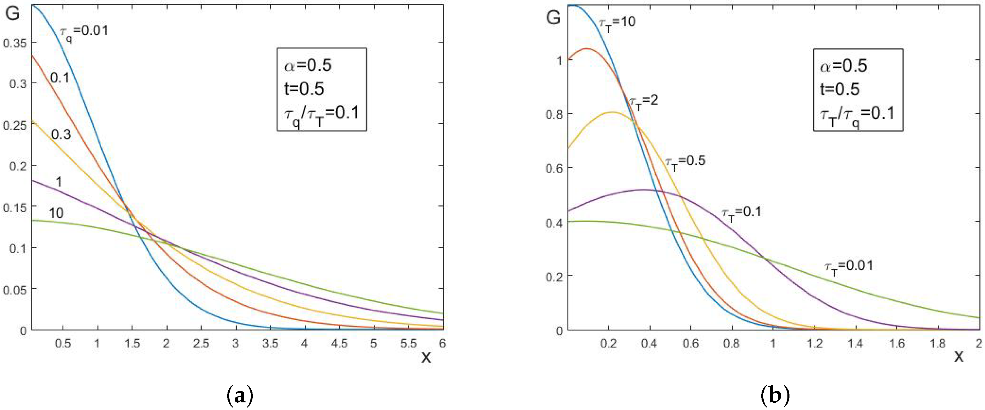
In
Figure 3 several plots are given with one and the same ratio of the relaxation times, in (a)
—diffusion regime; in (b)
—propagation regime. It is seen that different plots correspond to one and the same ratio, that is the fundamental solution depends not only on the ratio of the relaxation times, but on their specific values.
In all figures we observe behavior, typical for a diffusion process for
: the fundamental solution is monotonically decreasing in
x for
, representing a unimodal p.d.f. For
the behavior is typical for a propagation process, with a maximum moving away from the origin. In this respect there is a strong analogy with the fractional diffusion-wave equation with Caputo time-derivative of order
with the two corresponding regimes: diffusion (
) and propagation (
), c.f. ([
35] Figure 6.1), [
31].
6. Subordination Principles and Multi-Dimensional Fundamental Solutions
In this section, we give one more standard representation of the fractional Jeffreys-type heat conduction Equation (
15)—as a Volterra integral equation—and use some facts from the theory in the monograph [
38]. As in the beginning of this work we consider again Equation (
15) in general form without specifying the domain of the Laplace operator (finite or infinite spatial domain and type of boundary conditions). By the use of (
7) Equation (
15) reads in Laplace domain
where
. Taking the inverse Laplace transform in (
45) yields the Volterra integral equation
with kernel
satisfying
, where the function
is defined in (
36). The explicit representation for the kernel is deduced by the use of the Laplace transform pair (
11) as
Let us note that
. Indeed, according to (
12), the first derivative of
is
Therefore, for the function is decreasing from to and for the function is increasing from to .
Let us look briefly at propagation speed of a disturbance in model (
46). From general theory, see ([
38] Chapter 5), the velocity of propagation of the head of a disturbance is
Therefore,
, except in the special case
,
,
, in which we recognize the classical Cattaneo’s equation. Therefore, with the exception of this specific case, a disturbance propagates with infinite speed, and therefore the Equation (
15) is parabolic.
Let us point out that the symbol
in (
46) can represent different realizations of the Laplace operator, such that it is a closed and densely defined operator in the chosen space of functions and the wave equation
is well posed. For details on abstract Volterra integral equations we refer [
38]. Thanks to the properties of the function
given in Proposition 2 above, we can apply Theorems 4.2 and 4.3 in [
38] and formulate the following subordination principles. For completeness we briefly present the main idea and steps of the proof.
Theorem 3. The solution of Equation (46) satisfies the following subordination relationwhere the function is the solution of the classical wave equationand the kernel is defined via the Laplace transform In the diffusion case the following stronger subordination relation holds truewhere is the solution of the classical diffusion equationand the kernel is defined via the Laplace transform The functions , , are probability densities in τ, that is Proof. By applying Laplace transform in (
46) it follows
where the function
is defined in (
36) and
,
, denotes the resolvent operator of the operator
. It follows by the uniqueness of the Laplace transform that
is the solution of Equation (
46) if and only if identity (
53) is satisfied. So, our first aim is to prove that the functions defined by (
48) and (
50) satisfy (
53).
Consider first the function
defined by (
48). It is known (and easy to check) that the solution
of the wave equation obeys in Laplace domain
Then application of the Laplace transform in (
48) yields by the use of (
49) and (
54) with
Consider now the function
defined by (
50). The solution
of the diffusion equation obeys in Laplace domain
Therefore, application of the Laplace transform in (
50) yields by the use of (
51) and (
56) with
It remains to check properties (
52). The proof is analogous to that of Theorem 1. To prove non-negativity, it suffices to establish that
,
. The nonnegativity of
is already proved in Theorem 1,
is treated in an analogous way, taking into account that
for
.
Further, from the definitions (
49) and (
51) of the kernels
,
we obtain by the use and the Bromwich inversion formula
Therefore, the kernels are normalized and properties (
52) are established. □
Theorem 3 provides a useful tool for the study of multi-dimensional problems for Equation (
15) or problems on finite spatial domain by deriving the solution and relevant properties from known results concerning the corresponding diffusion and wave equations. An example of application of Theorem 3 is given next.
Theorem 4. For , , the fundamental solutions , , are spatial probability density functions evolving in time.
Proof. According to Theorem 3 subordination identity (
50) holds true. Therefore
where
is the Gaussian function given in (
38), for which it is well known that it is a spatial p.d.f. Therefore, the non-negativity of
imply directly the non-negativity of
and
where for the last identity we have used (
52). This proves the theorem. □
In contrast to Theorem 4, in the propagation case
the multi-dimensional fundamental solutions can have negative values. Next we give an example. Let us invert the Fourier transform in (
37) by the use of the inversion formula for the radial function
(see, e.g., [
34]) and formula 11.4.44 in [
39]
where
,
and
denote the Bessel function of the first kind and the modified Bessel function of the second kind, respectively, see [
39]. In the simplest multi-dimensional case,
, in which the inverse Fourier transform is expressed in terms of
, we deduce from (
37) the following expression for the Laplace transform of the fundamental solution
Comparing this result to (
39) we easily derive the following relation between
and
:
where
. Note that such a relation is already known for the case of fractional diffusion-wave equation with Caputo time-derivative,
, see, e.g., [
31]. Identity (
59) implies that
if and only if
is non-increasing for all
. However,
Figure 1b,
Figure 2b and
Figure 3b show that in the propagation case (
) the solution increases near the origin. This means that when (
) the three-dimenstional solution admits negative values.
To prove strictly that
can have negative values it suffices to show that
with respect to
s (Bernstein’s theorem). From (
58) we deduce the asymptotic expansion
which is not a completely monotone function with respect to
s provided
. Indeed, in this case its first derivative
as
and, thus,
as a function of
s does not satisfy inequalities (
13).
7. Concluding Remarks
The heat conduction equation with a fractional Jeffreys-type constitutive law is studied. By employing the Bernstein functions technique, two fundamentally different types of behavior are established, depending on the value of the characteristic parameter : diffusion regime for and propagation regime for . The one-dimensional fundamental solution is shown to be a spatial probability density function evolving in time, which is unimodal in the diffusion regime and bimodal in the propagation regime. The multidimensional fundamental solutions are probability densities only in the diffusion case, while in the propagation case they may have negative values.
The fractional Jeffreys-type heat conduction equation in the two different regimes is represented as a generalized diffusion, respectively wave, equation. The memory kernel in both cases is expressed in terms of Mittag–Leffler functions. The kernel is singular in the diffusion regime if and regular in the propagation regime. This shows that one and the same model may support different types of kernels.
Subordination principles are formulated, which are useful for the study of multi-dimensional problems on finite or infinite spatial region.
All results hold true also for the case of classical Jeffreys-type heat conduction equation ().
The established properties indicate a strong analogy between the fractional Jeffreys-type equation and the fractional diffusion-wave equation with the Caputo fractional time-derivative
with its two different regimes: diffusion (
) and propagation (
).
The technique developed in this work can be extended to the case of generalized diffusion-wave equation with a general memory kernel.


