Article

Dynamic Analysis of the Viscoelastic Pipeline Conveying Fluid with an Improved Variable Fractional Order Model Based on Shifted Legendre Polynomials

1
College of Sciences, Yanshan University, Qinhuangdao 066004, China
2
LE STUDIUM RESEARCH FELLOW, Loire Valley Institute for Advanced Studies, 45000 Orléans, France
3
INSA Center Val de Loire-88, Boulevard Lahitolle, 18000 Bourges, France
*
Author to whom correspondence should be addressed.
Fractal Fract. 2019, 3(4), 52; https://doi.org/10.3390/fractalfract3040052
Submission received: 10 October 2019 / Revised: 6 November 2019 / Accepted: 14 November 2019 / Published: 17 November 2019
(This article belongs to the Special Issue 2019 Selected Papers from Fractal Fract’s Editorial Board Members)

Abstract

:
Viscoelastic pipeline conveying fluid is analyzed with an improved variable fractional order model for researching its dynamic properties accurately in this study. After introducing the improved model, an involuted variable fractional order, which is an unknown piecewise nonlinear function for analytical solution, an equation is established as the governing equation for the dynamic displacement of the viscoelastic pipeline. In order to solve this class of equations, a numerical method based on shifted Legendre polynomials is presented for the first time. The method is effective and accurate after the numerical example verifying. Numerical results show that how dynamic properties are influenced by internal fluid velocity, force excitation, and variable fractional order through the proposed method. More importantly, the numerical method has shown great potentials for dynamic problems with the high precision model.

1. Introduction

Pipelines conveying fluid are of the significant structures in engineering and science fields, and they are involved in projects of heat exchanger devices, nuclear industries, oil transportation, cosmonautics, aviation, and hemodynamics. Due to the external load excitations, the internal fluid flowing, and other factors, the dynamic properties of the pipeline change. These will bring an uncertainty of the pipeline conveying fluid on engineering performance.
For the above reason, the dynamic analysis of infusion pipelines has always been the research hot spot and focus on the field of engineering and science. Peng et al. [1] studied the pipeline with inclined support to transport fluid. The dynamic analysis was carried out in the form of bifurcation diagram and oscillation trajectory, and the influence of system parameters on the performance of the system was studied. Chang and Sadeghi [2] studied cantilever pipes with and without end mass under small amplitude excitation. The influence of force excitation with different velocities, amplitudes, and frequencies on the pipeline was analyzed. He et al. [3] considered the elastic slender pipe and uniform transverse flow that transported the fluid under the excitation of the top force. The results show that the internal fluid velocity and external force play a key role in suppressing vortex-induced vibration. Rahmati et al. [4] focused on how the flow rate affects the stability of the pipeline in which the fluid is transported. However, most studies only focused on the influence of system parameters on stability. Zhang et al. [5] analyzed the chaotic dynamics of the pipeline conveying pulsating fluid under external loads. It is worth noting that it is dangerous to induce chaotic vibration of the above pipes. Zhang and Chen [6] studied the internal and external resonance dynamics of the pipeline conveying fluid under the action of nonlinear force. Wang et al. [7] studied the effects of several physical and geometric parameters on the dynamic characteristics of infusion pipelines by using bifurcation diagram and phase diagram. Tang et al. [8] considered a free vibration of viscoelastic pipes conveying fluid by a nonlinear fractional model and also investigated the effect of model parameters on the amplitudes and frequencies of pipes. Although a lot of research results have been contributed, there are still difficult problems in pipes conveying fluid aspects.
Several viscoelastic materials are widely used in fluid pipelines because of their damping and simulation of biological tissue. Mitsotakis et al. [9] considered viscoelastic wall tubes with pulsating flow, which is helpful to the simulation of hemodynamics. Yano et al. [10] studied viscoelastic materials as damped pipes to reduce vibration. In addition, due to the accurate model of viscoelastic constitutive relation, the dynamic analysis of viscoelastic pipelines has always been the key and a difficult problem of the infusion pipeline.
In the early studies, the viscoelastic constitutive model was described by integer order differential operators. Husain and Anderssen [11] considered Boltzmann model and Kohlrausch function to simulate the relaxation modulus of linear viscoelasticity. Yan et al. [12] selected a Kelvin–Voigt model to represent the character of viscoelastic interfaces. Machiraju et al. [13] used a generalized standard linear solid model to describe the stress relaxation modulus of human subscapular tendons. With the rapid development of fractional differential operators, fractional models are used in viscoelastic constitutive relations. Compared with integer order differential operators, fractional order differential operators can always better describe the memory properties of viscoelastic materials. The results in [14] show that the fractional model can simulate the viscoelastic constitutive relation well, has higher accuracy and less input parameters, and can adapt to the complex nonlinear viscoelastic behavior. Therefore, the fractional model begins to be applied to the dynamics of viscoelastic fields. Four kinds of fractional viscoelastic constitutive models were proposed in [15]. They are fractional Maxwell model, fractional Kelvin–Voigt model, fractional Zener model, and fractional Poynting–Thomson model, which are widely used to describe viscoelastic behavior. The fractional Zenner constitutive model [16] was applied to sandwich cylindrical shells. The influence of system parameters on flutter was analyzed. Yu et al. [17] used the generalized fractional model to describe the viscoelastic relaxation characteristics of soft tissue. In addition, the model was also used to simulate the flow structure interaction of patient-specific cerebral aneurysms. The results show that the fractional model can effectively simulate the complex dynamic behavior of viscoelastic materials. However, in most cases, the fractional model can not well describe the dynamic viscoelastic behavior. In the dynamic analysis, the slight change of the parameters will cause the great change of the system. Under the condition of large strain, the variable fractional order differential operator is better than the fractional order differential operator to simulate the viscoelastic constitutive relation [18]. For the accurate modeling of the viscoelastic constitution relation, a variable fractional order model was proposed. Meng et al. [19] investigated the compression deformation of amorphous glassy polymers with the variable fractional order model. The results demonstrated that the model has the advantages of higher accuracy and fewer parameters.
However, there is little research on the variable fractional order model of viscoelastic pipes. In order to improve the accuracy and efficiency of dynamic analysis, this study not only takes the variable fractional order model as the constitutive model of viscoelastic infusion pipelines, but also needs a reliable technique to accurately solve the variable fractional equation. Moreover, the governing equation is a class of variable fractional order, which is a nonlinear piecewise function containing analytic functions, differential equations. In recent years, researchers have studied numerical methods for various fractional differential equations. Sene et al. [20] used a homotopy perturbation ρ -Laplace transform method to study fractional diffusion and diffusion–reaction equations. Baleanu et al. [21] solved the Helmholtz equation based on local fractional derivative operators. Malmir [22] applied a new fractional integration operational matrix of Chebyshev wavelets to solve fractional delay equations. A Bernstein polynomial numerical method for solving a class of variable fractional order linear cable equations [23] and variable order time fractional diffusion equations [24] was proposed. For nonlinear fractional differential equations, a Legendre wavelet method was proposed to solve a class of nonlinear fractional differential equations [25] with nonlinear variables. Chen et al. [26] studied the Bernstein polynomials of a class of fractional differential equations with nonlinear variables by using the polynomial method. However, there are few studies on the numerical solutions of variable fractional order, which is nonlinear piecewise function containing analytic functions differential equations.
For these reasons, the variable fractional order model and a new method need to be applied to these kinds of problems in order to improve the accuracy and diversity of the solutions. In order to solve this problem numerically, an algorithm is proposed in this paper. The algorithm is not only suitable for solving the governing equations of variable fractional order models with higher accuracy, but also for the dynamic analysis of viscoelastic pipelines as a high precision technique. More importantly, this study will improve the reliability of predicting viscoelastic behavior and dynamic characteristics of flow pipeline.
The nonlinear dynamic analysis of viscoelastic pipeline under external load excitation is studied in this paper. In the next section, the variable fractional order model is selected as the constitutive model to derive the governing equation of the pipeline. In addition, it is a form of nonlinear differential equations with variable fractional order which is a nonlinear piecewise function containing analytic functions. In the third section, the Shift Legendre Polynomial algorithm is proposed to obtain the numerical solution of the pipeline governing equation. In the fourth section, the effects of various parameters on pipeline dynamics are studied. Finally, the fifth section gives the conclusion.

2. Mathematical Model

2.1. Mathematical Preliminaries

Here, several mathematical preliminaries on fractional order derivatives are introduced and they are applied in the following sections.
Definition 1.
The Caputo fractional derivative operator D α ( x , t ) of order α ( x , t ) is defined as [22,26]
D α ( x , t ) f ( t ) = 1 Γ ( 1 α ( x , t ) ) 0 + t ( t τ ) α ( x , t ) f ( τ ) d τ ,
where t 0 , 0 < α ( x , t ) 1 , and α ( x , t ) is variable fractional order, f ( t ) is continuous over interval ( 0 , + ) , and is integrable over any subinterval of [ 0 , + ) .
According to Definition 1, the variable fractional derivative of a polynomial can be expressed as
D t α ( x , t ) t n = Γ ( n + 1 ) Γ ( n + 1 α ( x , t ) ) t n α ( x , t ) , n = 1 , 2 , 0 , n = 0 .
This property facilitates the algorithm proposed later.

2.2. Motion Equation of Viscoelastic Pipeline Conveying Fluid

A viscoelastic pipeline conveying fluid internal fluid, which is simply supported at both ends, is considered in this section, as shown in Figure 1. The model applied in this research is composed of fluid and structure parts. Without considering internal damping and gravity effects, the governing equation can be derived by constitutive model [18] and Hamilton’s principle and expressed as
E I θ α 4 + α w x 4 t α + ( m f V f 2 T 0 ) 2 w x 2 + 2 m f V f 2 w x t + ( m p + m f ) 2 w t 2 = f ,
where E and θ are parameters of the constitutive model, I is the area moment of inertia, T 0 is the tensional force which is a constant, H is the length of the pipeline, m p and m f are respectively the mass per unit length of the pipeline and internal fluid, V f is the internal fluid velocity, f is the force excitation per unit length, and w is the transverse displacement of pipeline.
The fractional order α is a constant at the time of small deformation and a linear function with respect to strain at the time of large deformation. Under the force excitation, the strain of viscoelastic pipeline is varying continuously between large deformation and small deformation. For accurately describing the constitutive relationship of viscoelastic pipelines, the following variable fractional order model, which is both suitable for small deformation and large deformation, is selected in this work.
α = α 0 , ε α b , α 0 α k ( ε α b ) , ε > α b ,
where α is fractional order, which must satisfy 0 < α < 1 , α 0 , α k and α b are parameters of α , and ε is the strain of viscoelastic pipeline.
In addition, the strain can be formulated as
ε = 1 2 ( w x ) 2 ,
where w is displacement of viscoelastic pipeline. Then, fractional order α can be written as
α = α 0 , 1 2 ( w x ) 2 α b , α 0 α k 1 2 ( w x ) 2 α b , 1 2 ( w x ) 2 > α b .
It notes the fractional order is a constant when strain 1 2 ( w x ) 2 is less than or equal to a value α b and a nonlinear function when 1 2 ( w x ) 2 is more than a value α b .
Finally, the governing equation for the viscoelastic pipeline conveying fluid is formulated as
E I θ α 4 + α w x 4 t α + ( m f V f 2 T 0 ) 2 w x 2 + 2 m f V f 2 w x t + ( m p + m f ) 2 w t 2 = f , α = α 0 , 1 2 ( w x ) 2 α b , α 0 α k 1 2 ( w x ) 2 α b , 1 2 ( w x ) 2 > α b .
The boundary conditions are
ω ( 0 , t ) = 0 , ω ( H , t ) = 0 , w ( 0 , t ) x = 0 , w ( H , t ) x = 0 .

3. Numerical Study

In this section, a numerical method is proposed to solve this class of variable fractional equations on the basis of shifted Legendre polynomials. Then, the specific process is shown in the following section.

3.1. Shifted Legendre Polynomials

Legendre polynomial is an orthogonal polynomial used to approximate analytical solution as the basic function. However, the Legendre polynomial can’t satisfy the physical significance in many engineering and science problems due to its definition range [ 1 , 1 ] . For overcoming this problem, the shifted Legendre polynomial is introduced. The shifted Legendre polynomials of degree n in [ 0 , 1 ] [25] is defined as
L G n , i ( x ) = i = 0 n ( 1 ) n + i Γ ( n + i + 1 ) Γ ( n i + 1 ) ( Γ ( i + 1 ) ) 2 x i ,
where i = 0 , 1 , , n , x [ 0 , 1 ] . Then, a sequence Legendre polynomial matrix Φ n ( x ) is formulated as
Φ n ( x ) = [ L G n , 0 ( x ) , L G n , 1 ( x ) , , L G n , n ( x ) ] T , Φ n ( x ) = A T n ( x ) ,
where T n ( x ) = [ 1 , x , , x n ] T ,
A = [ a i j ] i , j = 0 n , a i j = 0 , i < j , ( 1 ) i + j Γ ( i + j + 1 ) Γ ( i j + 1 ) ( Γ ( j + 1 ) ) 2 , i j .
In order to expand the range of x, the shifted Legendre polynomial of degree n in [ 0 , L ] is formulated as
L G L n , i ( x ) = i = 0 n ( 1 ) n + i Γ ( n + i + 1 ) Γ ( n i + 1 ) ( Γ ( i + 1 ) ) 2 x L i , = i = 0 n ( 1 ) n + i Γ ( n + i + 1 ) Γ ( n i + 1 ) ( Γ ( i + 1 ) ) 2 1 L i x i ,
where i = 0 , 1 , , n , x [ 0 , L ] . Then, a sequence of shifted Legendre polynomials matrix Φ L n ( x ) is formulated as
Φ L n ( x ) = A L T n ( x ) ,
where
L = [ l i j ] i , j = 0 n , l i j = 0 , i j , L i , i = j .
The shifted Legendre polynomial of degree n in [ 0 , S ] is formulated as
L G S n , i ( t ) = i = 0 n ( 1 ) n + i Γ ( n + i + 1 ) Γ ( n i + 1 ) ( Γ ( i + 1 ) ) 2 t S i , = i = 0 n ( 1 ) n + i Γ ( n + i + 1 ) Γ ( n i + 1 ) ( Γ ( i + 1 ) ) 2 1 S i t i ,
where i = 0 , 1 , , n , t [ 0 , S ] . Then, a sequence shifted Legendre polynomial matrix Φ s n ( t ) is defined as
Φ s n ( t ) = A M T n ( t ) ,
where
M = [ m i j ] i , j = 0 n , m i j = 0 , i j , S i , i = j .

3.2. Function Approximation

A continuous function W ( x ) in the domain [ 0 , L ] can be expanded in terms of shifted Legendre polynomials as W ( x ) = lim n i = 0 n c i L G L n , i ( x ) , W ( x ) can be approximated as
W ( x ) W n ( x ) = i = 0 n c i L G L n , i ( x ) = C T Φ L n ( x ) ,
where C T = [ c 0 , c 1 , , c n ] is an unknown coefficient matrix. Let
C T Φ L n ( x ) , Φ L n T ( x ) = u ( x ) , Φ L n T ( x ) .
Then,
C T = u ( x ) , Φ L n ( x ) Q 1 ,
where Q = Φ L n , Φ L n T ( x ) = [ δ i j ] i , j = 0 n , δ i j = 0 L L n , i ( x ) L n , j ( x ) d x = 0 , i j L i + j + 1 , i = j , ( i , j = 0 , 1 , , n ) .
Similarly, a continuous function W ( t ) in the domain [ 0 , S ] can be expanded in terms of shifted Legendre polynomials as W ( t ) = lim n i = 0 n k i L G S n , i ( t ) , W ( t ) can be approximated as
W ( t ) W n ( t ) = i = 0 n k i L G S n , i ( t ) = K T Φ L n ( t ) ,
where K T = [ k 0 , k 1 , , k n ] is an unknown coefficient matrix. Let
K T Φ L n ( t ) , Φ L n T ( t ) = W ( t ) , Φ L n T ( t ) .
Then,
K T = W ( t ) , Φ L n T ( t ) R 1 ,
where R = Φ L n ( t ) , Φ L n T ( t ) = [ Δ i j ] i , j = 0 n , Δ i j = 0 S L G S n , i ( t ) L G S n , j ( t ) d t = 0 , i j S i + j + 1 , i = j ( i , j = 0 , 1 , , n ) .
Two-variable continuous function W ( x , t ) L 2 [ 0 , H ] × [ 0 , S ] can be formulated as
W ( x , t ) = lim n j = 0 n ( i = 0 n c i L G L n , i ( x ) ) k j L G S n , j ( t ) = lim n j = 0 n i = 0 n c i k j L G L n , i ( x ) L G S n , j ( t ) = lim n j = 0 n i = 0 n Λ i j L G L n , i ( x ) L G S n , j ( t ) = lim n Λ T [ Φ L n ( x ) Φ S n ( t ) ] ,
where Λ = [ Λ 00 , Λ 01 , , Λ 0 n , Λ 10 , Λ 11 , , Λ 1 n , , Λ n 0 , Λ n 1 , , Λ n n ] T is an unknown coefficient matrix, Λ = C K , and ⊗ is Kronecker product.

3.3. Differential Operator Matrix

Φ L n ( x ) is a sequence of polynomials matrix with respect to x, the derivative of Φ L n ( x ) with respect to x is formulated as
d Φ L n ( x ) d x = B x Φ L n ( x ) .
Then,
B x Φ L n ( x ) = B x A L T n ( x ) = A L d T n ( x ) d x = A L F T n ( x ) = A L F ( A L ) 1 Φ L n ( x ) ,
where F = [ f i j ] i , j = 0 n , f i j = 0 , i j + 1 , i , i = j + 1 .
From formula (23), one exponent t h differential operator matrix with respect to x is obtained as
B x = A L F ( A L ) 1 .
The m exponent t h derivative of Φ L n ( x ) with respect to x is formulated as
d m Φ L n ( x ) d x m = B m x Φ L n ( x ) , m N .
Then,
B m x Φ L n ( x ) = B m x A L T n ( x ) = A L d m T n ( x ) d x m = A L F m T n ( x ) = A L F m ( A L ) 1 Φ L n ( x ) .
Based on formula (26), m exponent t h differential operator matrix with respect to x can be given as
B m x = A L F m ( A L ) 1 .
Similarly, Φ S n ( t ) is a sequence of polynomials matrix with respect to t, the derivative of Φ S n ( t ) with respect to t is formulated as
d Φ S n ( t ) d t = B t Φ S n ( t ) .
Then,
B t Φ S n ( t ) = B t A M T n ( t ) = A M d T n ( t ) d t = A M F T n ( t ) = A M F ( A M ) 1 Φ S n ( t ) .
Therefore, from (29), one exponent t h differential operator matrix with respect to t is obtained as
B t = A M F ( A M ) 1 .
The v exponent t h derivative of Φ S n ( t ) with respect to t is formulated as
d v Φ S n ( t ) d t v = B v t Φ S n ( t ) , v N .
Then, we have
B v t Φ S n ( t ) = B v t A M T n ( t ) = A M d v T n ( t ) d t v = A M F v T n ( t ) = A M F v ( A M ) 1 Φ S n ( t ) .
Based on Formula (32), v exponent t h differential operator matrix with respect to x is obtained as
B v t = A M F v ( A M ) 1 .
The α exponent t h derivative of Φ S n ( t ) with respect to t is formulated as
d α Φ S n d t α = B α t Φ S n ( t ) , α ( 0 , 1 ) ,
B α t Φ S n ( t ) = B α t A M T n ( t ) = A M d α T n ( t ) d t α = A M G T n ( t ) = A M G ( A M ) 1 Φ S n ( t ) ,
where G = [ g i j ] i , j = 0 n , g i j = Γ ( i + 1 ) Γ ( i + 1 α ) t α , i = j , i 1 , 0 , o t h e r w i s e . Then, α exponent t h differential operator matrix with respect to t can be expressed as
B α t = A M G ( A M ) 1 .
Thus,
m + v W ( x , t ) x m t v Λ T ( B m x Φ L n ( x ) ) ( B v t Φ S n ( t ) ) ,
m + α W ( x , t ) x m t α Λ T ( B m x Φ L n ( x ) ) ( B α t Φ S n ( t ) ) ,
where Λ is an unknown coefficient matrix.
Finally, the governing equation will be converted into the following algebraic equation:
E I θ α Λ T ( B 4 x Φ L n ( x ) ) ( B α t Φ S n ( t ) ) + ( m f V f 2 T 0 ) Λ T ( B 2 x Φ L n ( x ) ) Φ S n ( t ) + 2 m f V f Λ T ( B x Φ L n ( x ) ) ( B t Φ S n ( t ) ) + ( m p + m f ) Λ T Φ L n ( x ) ( B t Φ S n ( t ) ) = f , α = α 0 , 1 2 Λ T ( B 2 x Φ L n ( x ) ) Φ S n ( t ) 2 α b , α 0 α k 1 2 Λ T ( B 2 x Φ L n ( x ) ) Φ S n ( t ) 2 α b , 1 2 Λ T ( B 2 x Φ L n ( x ) ) Φ S n ( t ) 2 > α b .
Discreting x and t, Λ is obtained. In addition, solution w ( x , t ) is obtained.

3.4. Numerical Example

Consider the following variable fractional equation:
2 α 4 + α w ( x , t ) x 4 t α + 2 w ( x , t ) x 2 + 2 w ( x , t ) x t + 2 w ( x , t ) t 2 = q ( x , t ) , α = 0.56 , ( w ( x , t ) x ) 2 0.01 , 0.56 0.1 ( w ( x , t ) x ) 2 0.01 , ( w ( x , t ) x ) 2 > 0.01 ,
where
q ( x , t ) = 2 α 24 Γ ( 3 ) Γ ( 3 α ) t 2 α + ( 12 x 2 12 x + 2 ) t 2 + ( 8 x 3 12 x 2 + 4 x ) t + 2 x 2 ( 1 x ) 2 .
The exact solution w ( x , t ) can be expressed as
w ( x , t ) = x 2 ( 1 x ) 2 t 2 , x [ 0 , 1 ] , t [ 0 , 2 ] .
The boundary conditions are
w ( 0 , t ) = w ( 1 , t ) = w ( 0 , t ) x = w ( 1 , t ) x = 0 .
The numerical solution w n ( x , t ) is obtained by the above method for n values 5. The absolute error is written as e w ( x , t ) = | w n ( x , t ) w ( x , t ) | , which is shown in Figure 2a. In addition, the comparison of numerical solution w n ( x , t ) is shown in Figure 2c. As can be seen in Figure 2b, the range of ( w ( x , t ) x ) 2 , which determines fractional order α ( x , t ) is a constant or an unknown piecewise nonlinear function for analytical solution, is [0,0.6], Then, α ( x , t ) is an unknown piecewise nonlinear function for analytical solution and satisfies 0 < α ( x , t ) < 1 . These indicate the numerical solution and exact solution are highly consistent and the absolute error is less than 1 . 5 × 10 12 . Moreover, it is verified that the proposed numerical method is accurately and effectively for solving variable fractional order, which is an unknown piecewise nonlinear function for analytical solution, differential equations.

4. Numerical Results and Analysis

Dynamic response of viscoelastic pipeline conveying fluid is analyzed in this section. The ring-shaped pipeline is considered. The fixed parameters of viscoelastic pipeline and internal fluid are shown in Table 1.
The approximate solutions of the response for viscoelastic pipelines are shown in Figure 3a,b. Here, viscoelastic pipeline is analyzed when V f , f and α are considered as V f = 10 m / s , f = 200 sin ( 500 t ) N / m and α = 0.65 , 1 2 ( w x ) 2 0.6 , 0.65 0.2 1 2 ( w x ) 2 0.6 , 1 2 ( w x ) 2 > 0.6 . It can be seen that the dynamic response is fluctuating with time increasing, and one peak and two troughs occur in the middle of the pipeline. In addition, the displacement amplitude in the middle of the pipeline is the largest. It can be concluded that response frequency is far less than the force excitation frequency.
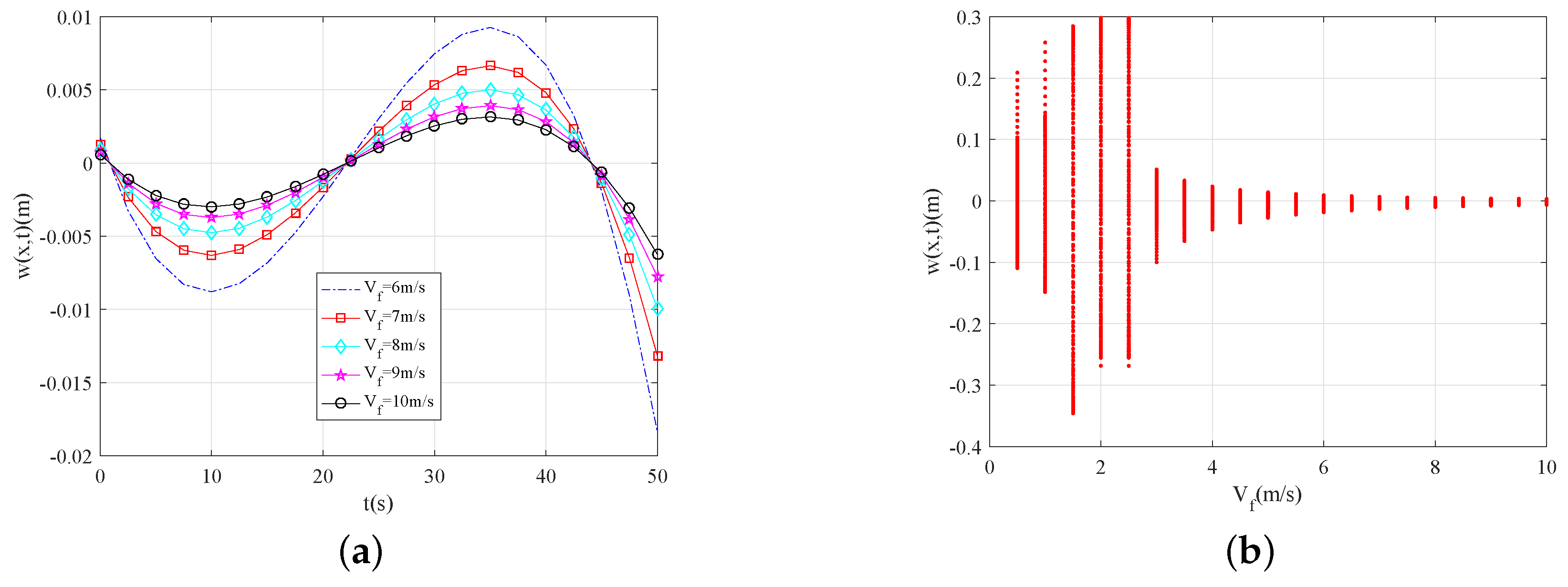
For investigating the effect of internal fluid velocity on response of pipeline, f and α are considered as f = 100 sin ( 500 t ) N / m and α = 0.65 , 1 2 ( w x ) 2 0.6 , 0.65 0.2 1 2 ( w x ) 2 0.6 , 1 2 ( w x ) 2 > 0.6 . As can be seen from Figure 4a, the displacement response amplitude is nonlinearly decreasing with internal fluid velocity linearly increasing from 6 m/s to 10 m/s. The response oscillation amplitude is increasing firstly and then decreasing with internal fluid velocity increasing shown in Figure 4b. It can be concluded that dynamic response amplitude is firstly decreasing and then nonlinearly increasing.
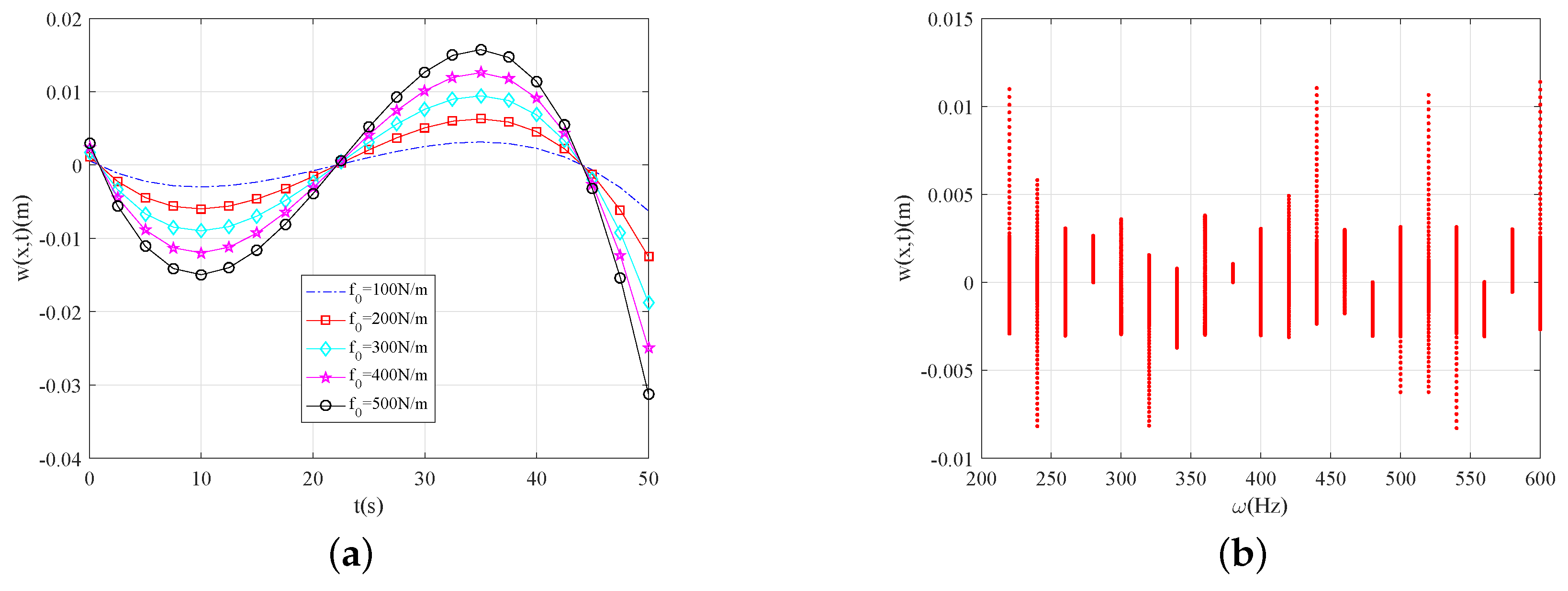
In order to research the effect of the force excitation on the pipeline, V f and α are considered as V f = 10 m/s and α = 0.65 , 1 2 ( w x ) 2 0.6 , 0.65 0.2 1 2 ( w x ) 2 0.6 , 1 2 ( w x ) 2 > 0.6 . It can be seen intuitively from Figure 5a,b that dynamic response amplitude is linearly increasing with the force excitation amplitude increasing, and irregularly changing with the force excitation frequency increasing.
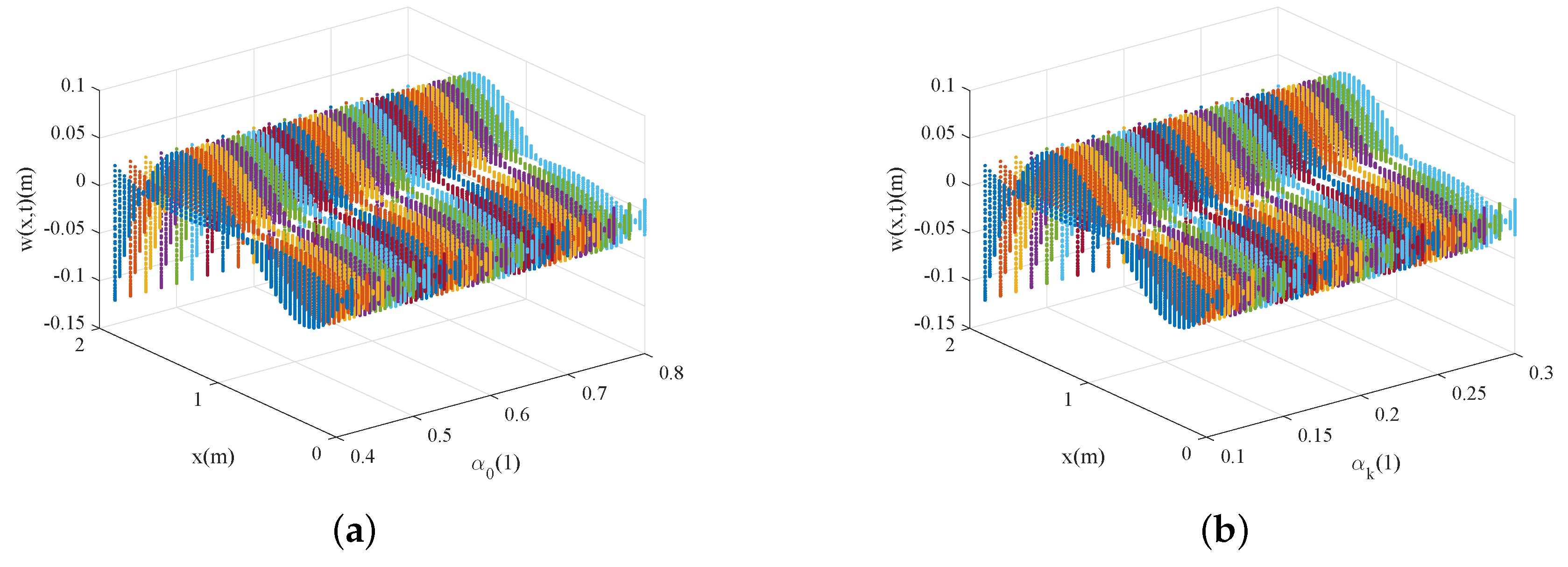
For researching the impact of variable fractional order on viscoelastic pipeline, V f and f are considered as V f = 10 m/s, f = 2000 sin ( 500 t ) N / m . As can be seen in Figure 6a,b, oscillation range is varying with position x and nearly varying with α 0 and α k . It can be concluded that changes in the variable fractional order have almost no effect on the oscillation range of the viscoelastic pipeline.

5. Conclusions

As the research concerning with the variable fractional order model applied on fluid-solid interaction is very little, dynamic properties for viscoelastic pipelines conveying fluid are studied in this paper. A class of variable fractional order, which is an unknown piecewise nonlinear function for analytical solution, equation is established as the more accurate governing equation than before and solved by the proposed numerical method based on shifted Legendre polynomials for the first time. After verifying, this algorithm is accurate and effective for solving these types of equations. The research yields the following conclusions on the basis of numerical results obtained by the numerical method:
(1) The dynamic response frequency of viscoelastic pipelines conveying fluid is far less than force excitation frequency.
(2) As the fluid velocity is increasing, the dynamic response amplitude is firstly increasing and then nonlinearly decreasing.
(3) The dynamic response amplitude of viscoelastic pipelines is linearly increasing with force excitation amplitude increasing and irregularly changing with the force excitation frequency increasing.
(4) Changes in the variable fractional order have almost no effect on the oscillation range of viscoelastic pipeline.

Author Contributions

Y.W. wrote some sections of the manuscript and performed analyses; Y.C. prepared some other sections of the paper. Both authors read and approved the final manuscript.

Funding

This work is supported by the Natural Science Foundation of Hebei Province (A2017203100) in China and the LE STUDIUM RESEARCH PROFESSORSHIP award of Centre-Val de Loire region in France.

Conflicts of Interest

The authors declare no conflict of interest.

References

  1. Peng, G.; Xiong, Y.M.; Liu, L.M.; Gao, Y.; Wang, M.H.; Zhang, Z. 3D nonlinear dynamics of inclined pipe conveying fluid supported at both ends. J. Sound Vib. 2019, 449, 405–426. [Google Scholar] [CrossRef]
  2. Chang, G.H.; Sadeghi, Y.M. Flow-induced oscillations of a cantilevered pipe conveying fluid with base excitation. J. Sound Vib. 2014, 333, 4265–4280. [Google Scholar] [CrossRef]
  3. He, F.; Dai, H.L.; Huang, Z.H.; Wang, L. Nonlinear dynamics of a fluid-conveying pipe under the combinedaction of cross-flow and top-end excitations. Appl. Ocean Res. 2017, 62, 199–209. [Google Scholar] [CrossRef]
  4. Rahmati, M.; Mirdamadi, H.R.; Goli, S. Divergence instability of pipes conveying fluid with uncertain flow velocity. Physica A 2018, 491, 650–665. [Google Scholar] [CrossRef]
  5. Zhang, Y.F.; Yao, M.H.; Zhang, W.; Wen, B.C. Dynamical modeling and multi-pulse chaotic dynamics of cantilevered pipe conveying pulsating fluid in parametric resonance. Aerosp. Sci. Technol. 2017, 68, 441–453. [Google Scholar] [CrossRef]
  6. Zhang, Y.L.; Chen, L.Q. External and internal resonances of the pipe conveying fluid in the supercritical regime. J. Sound Vib. 2013, 332, 2318–2337. [Google Scholar] [CrossRef]
  7. Wang, L.; Liu, Z.Y.; Abdelkefi, A.; Wang, Y.K.; Dai, H.L. Nonlinear dynamics of cantilevered pipes conveying fluid: Towards a further understanding of the effect of loose constraints. Int. J. Non-Linear Mech. 2017, 95, 19–29. [Google Scholar] [CrossRef]
  8. Tang, Y.; Zhen, Y.X.; Fang, B. Nonlinear vibration analysis of a fractional dynamic model for the viscoelastic pipe conveying fluid. Appl. Math. Model. 2018, 56, 123–136. [Google Scholar] [CrossRef]
  9. Mitsotakis, D.; Dutykh, D.; Li, Q.; Peach, E. On some model equations for pulsatile flow in viscoelastic vessels. Wave Motion 2019, 90, 139–151. [Google Scholar] [CrossRef]
  10. Yano, D.; Ishikawa, S.; Tanaka, K.; Kijimoto, S. Vibration analysis of viscoelastic damping material attached to a cylindrical pipe by added mass and added damping. J. Sound Vib. 2019, 454, 14–31. [Google Scholar] [CrossRef]
  11. Husain, S.A.; Anderssen, R.S. Modelling the relaxation modulus of linear viscoelasticity using Kohlrausch functions. J. Non-Newton. Fluid Mech. 2005, 125, 159–170. [Google Scholar] [CrossRef]
  12. Yan, W.; Ying, J.; Chen, W.Q. The behavior of angle-ply laminated cylindrical shells with viscoelastic interfaces in cylindrical bending. Compos. Struct. 2007, 78, 551–559. [Google Scholar] [CrossRef]
  13. Machiraju, C.; Phan, A.V.; Pearsall, A.W.; Madanagopal, S. Viscoelastic studies of human subscapularis tendon: Relaxation test and a Wiechert model. Comput. Methods Programs Biomed. 2006, 83, 29–33. [Google Scholar] [CrossRef] [PubMed]
  14. Peng, Y.; Zhao, J.Z.; Li, Y.M. A wellbore creep model based on the fractional viscoelastic constitutive equation. Pet. Explor. Dev. 2017, 44, 1038–1044. [Google Scholar] [CrossRef]
  15. Long, J.M.; Xiao, R.; Chen, W. Fractional viscoelastic models with non-singular kernels. Mech. Mater. 2018, 127, 55–64. [Google Scholar] [CrossRef]
  16. Mokhtari, M.; Permoon, M.R.; Haddadpour, H. Aeroelastic analysis of sandwich cylinder with fractional viscoelastic core described by Zener model. J. Fluids Struct. 2019, 85, 1–16. [Google Scholar] [CrossRef]
  17. Yu, Y.; Perdikaris, P.; Karniadakis, G.E. Fractional modeling of viscoelasticity in 3D cerebral arteries and aneurysms. J. Comput. Phys. 2016, 323, 219–242. [Google Scholar] [CrossRef]
  18. Meng, R.F.; Yin, D.; Drapaca, C.S. A variable order fractional constitutive model of the viscoelastic behavior of polymers. Int. J. Non-Linear Mech. 2019, 113, 171–177. [Google Scholar] [CrossRef]
  19. Meng, R.F.; Yin, D.; Drapaca, C.S. Variable-order fractional description of compression deformation of amorphous glassy polymers. Comput. Mech. 2019, 64, 163–171. [Google Scholar] [CrossRef]
  20. Sene, N.; Fall, A.N. Homotopy perturbation ρ-Laplace transform method and its application to the fractional diffusion equation and the fractional diffusion–reaction equation. Fractal Fract. 2019, 3, 14. [Google Scholar] [CrossRef]
  21. Baleanu, D.; Jassim, H.K.; Qurashi, M.A. Solving Helmholtz equation with local fractional derivative operators. Fractal Fract. 2019, 3, 43. [Google Scholar] [CrossRef]
  22. Malmir, I. A new fractional integration operational matrix of Chebyshev wavelets in fractional delay systems. Fractal Fract. 2019, 3, 46. [Google Scholar] [CrossRef]
  23. Chen, Y.M.; Liu, L.Q.; Li, B.F.; Sun, Y.N. Numerical solution for the variable order linear cable equation with Bernstein polynomials. Appl. Math. Comput. 2014, 238, 329–341. [Google Scholar] [CrossRef]
  24. Chen, Y.M.; Liu, L.Q.; Li, X.; Sun, Y.N. Numerical solution for the variable order time fractional diffusion equation with Bernstein polynomials. Comput. Model. Eng. Sci. 2014, 97, 81–100. [Google Scholar]
  25. Chen, Y.M.; Wei, Y.Q.; Liu, D.Y.; Yu, H. Numerical solution for a class of nonlinear variable order fractional differential equations with Legendre wavelets. Appl. Math. Lett. 2015, 46, 83–88. [Google Scholar] [CrossRef]
  26. Chen, Y.M.; Liu, L.Q.; Liu, D.Y.; Boutat, D. Numerical study of a class of variable order nonlinear fractional differential equation in terms of Bernstein polynomials. Ain Shams Eng. J. 2018, 9, 1235–1241. [Google Scholar] [CrossRef] [Green Version]
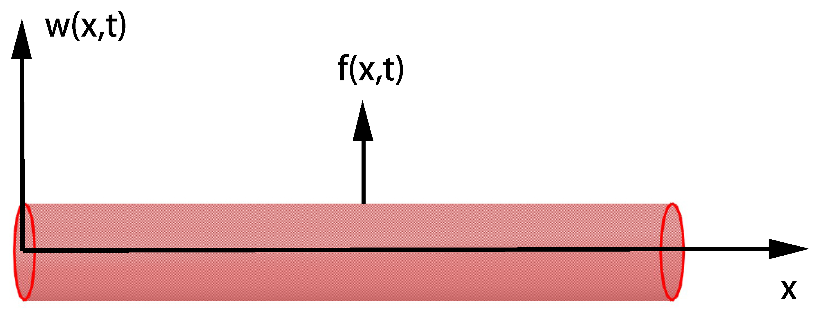
Figure 1. The geometric shape of viscoelastic pipeline.
Fractalfract 03 00052 g001
Figure 2. The numerical example results when n values 4 for (a) absolute error e w ( x , t ) , (b) ( w ( x , t ) x ) 2 , and (c) comparison of exact solution and numerical solution.
Fractalfract 03 00052 g002
Figure 3. Dynamic response on the viscoelastic pipeline conveying fluid when n values 4 within 50 s for (a) three-dimensional displacement map and (b) contour displacement map.
Fractalfract 03 00052 g003
Figure 4. Dynamic response with the fluid velocity varying when n values 4 and x values 1 m within 50 s for (a) displacement response of w ( x , t ) and (b) displacement oscillation of w ( x , t ) .
Fractalfract 03 00052 g004
Figure 5. Dynamic response with the force excitation varying when n values 4 and x values 1 m within 50 s for (a) excitation amplitude f 0 and (b) excitation frequency ω .
Fractalfract 03 00052 g005
Figure 6. Oscillation response with the variable fractional order varying when n values 4 within 50 s for (a) basic order α 0 and (b) order varying rate α k .
Fractalfract 03 00052 g006
Table 1. The fixed parameters of viscoelastic pipeline and internal fluid.
Physical QuantitySymbolValueDimension
External radiusD 0.4 m
Internal radiusd 0.32 m
LengthH2 m
Area moment of inertiaI 0.0119 m 4
Constitutive model parameterE600 MPa
Constitutive model parameter θ 0.1 1
Density of viscoelastic pipeline ρ p 1.2 × 10 3 kg · m 3
Density of internal fluid ρ f 1.05 × 10 3 kg · m 3
Mass per unit length of viscoelastic pipeline m p 217.2 kg · m 1
Mass per unit length of internal fluid m f 168.84 kg · m 1
Tensional force T 0 500 N