A New Fractional Integration Operational Matrix of Chebyshev Wavelets in Fractional Delay Systems

Abstract
:1. Introduction
2. Preliminaries
Useful Properties of CWs
- can be expressed in terms of by the integration operational matrix of CWs denoted by as
- the product operational matrix of CWs for denoted by the symbol simplifies to
- and , where is a time-delay and is a piecewise delay, are expressed by the delay and the piecewise delay operational matrices of CWs denoted by the symbols, in turn, and , where
- is expressed by the inverse (reverse) time operational matrix of CWs denoted by as
- is obtained as the integration matrix of the product of two CWs vectors on denoted by , that is,
3. The Fractional Integration Operational Matrix of CWs
4. Chebyshev Wavelet Methods for Fractional Delay Systems
4.1. Optimal Control of Linear-Quadratic Fractional Time-Delay Systems
4.2. Analysis of Linear Fractional Time-Delay Systems
5. Illustrative Examples
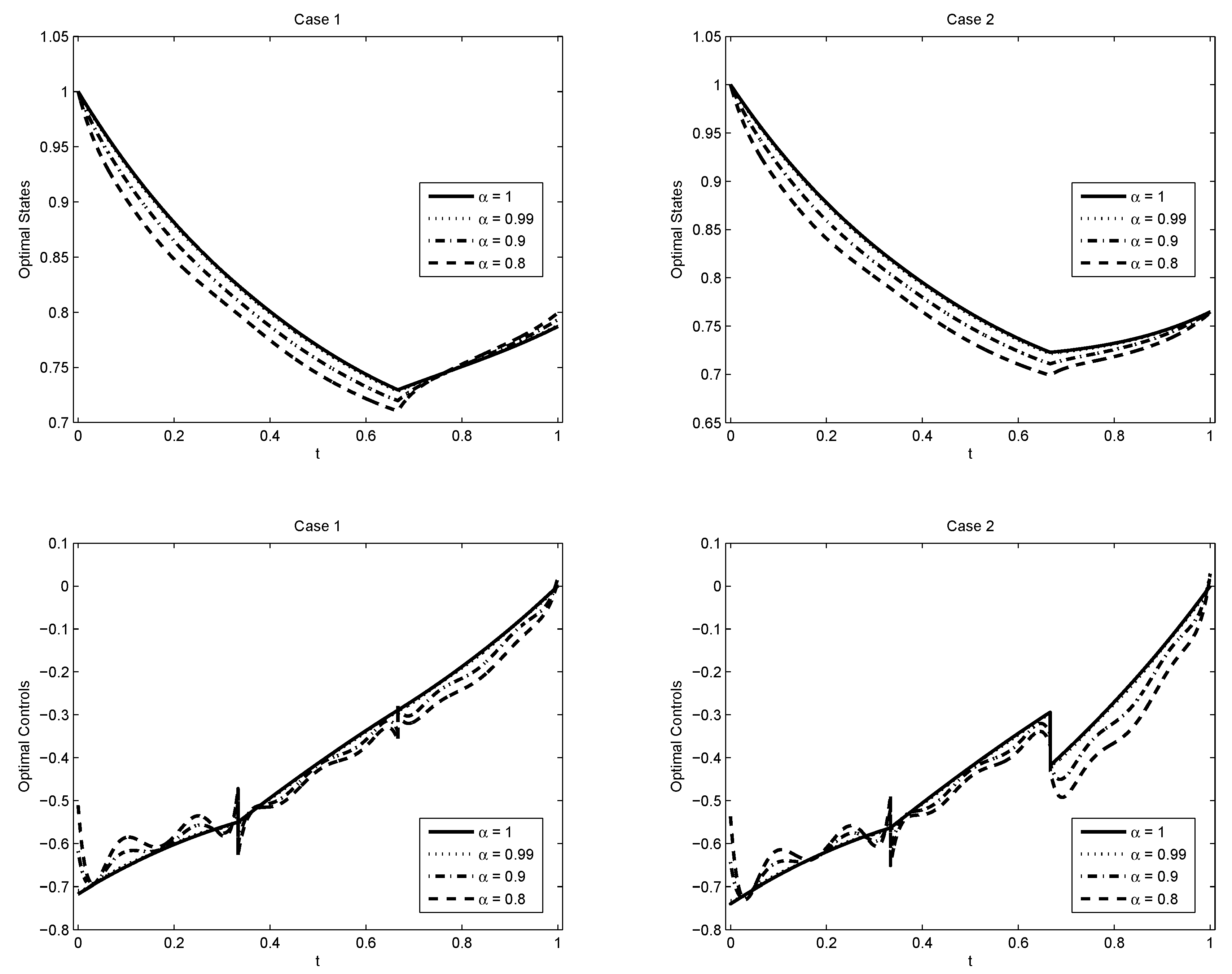
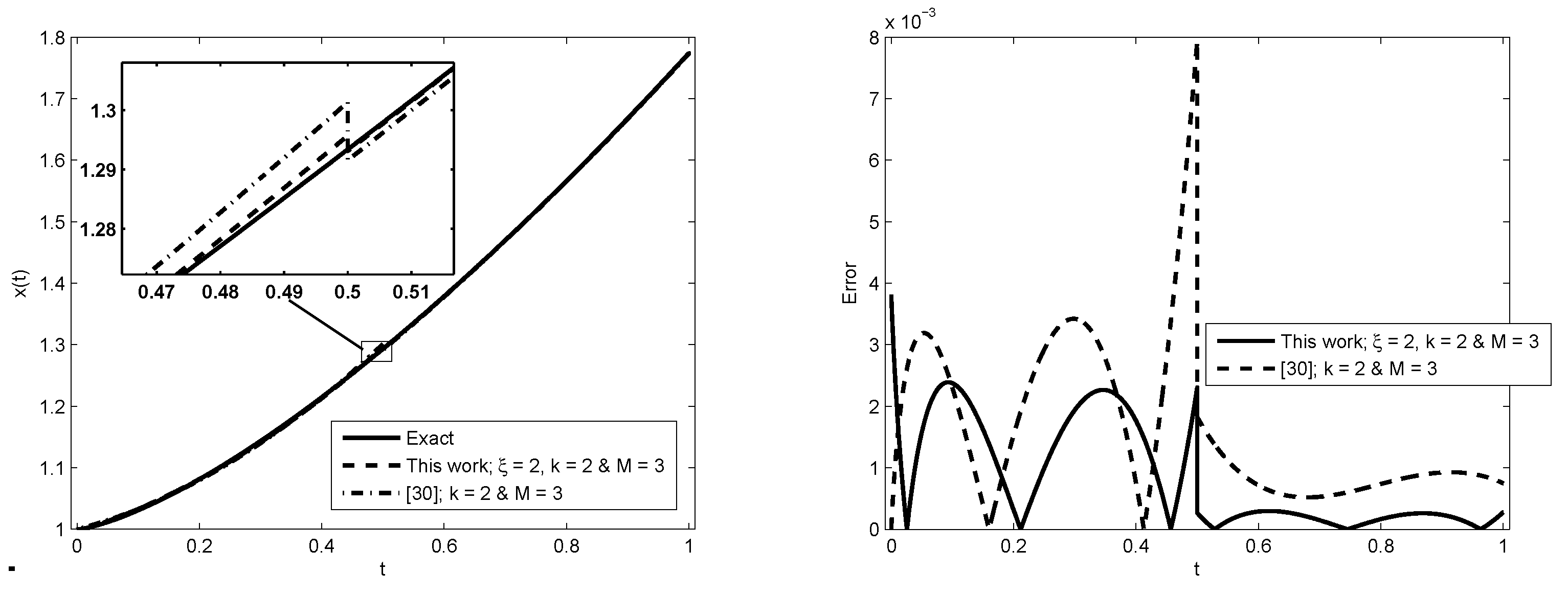
5.1. Example 1
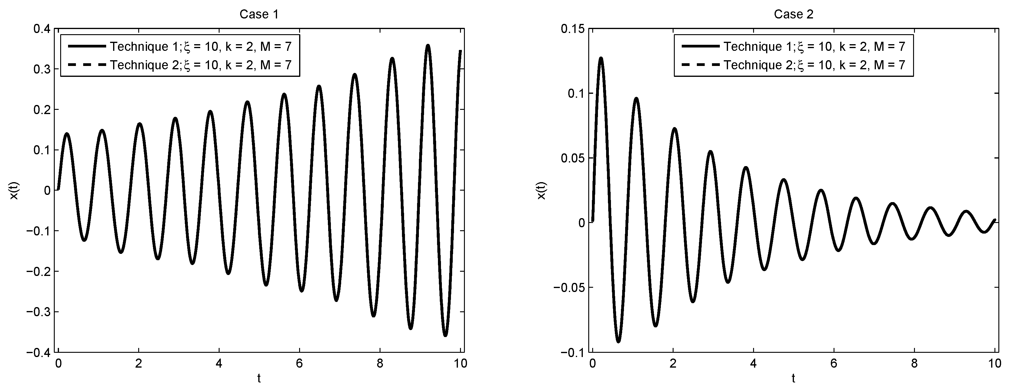
- Case 1:
- Case 2:
5.2. Example 2
5.3. Example 3
5.4. Example 4
5.5. Example 5
5.6. Example 6
- (1)
- We use the proposed method directly on this system;
- (2)
- By the technique used in [27], we first select the first derivative of as a new state which is , and set , then we solve the new problem aswhere is the corresponding initial function. In addition, we consider two cases.
- Case 1:
- and .
- Case 2:
- and .
5.7. Example 7
- Case 1:
- and the system is unconstrained.
- Case 2:
- and the path constraint is .
- Case 3:
- and the path constraint is .
6. Conclusions
Funding
Acknowledgments
Conflicts of Interest
References
- Miller, K.S.; Ross, B. An Ontroduction to the Fractional Calculus and Fractional Sifferential Equations; John Wiley & Sons: Hoboken, NJ, USA, 1993. [Google Scholar]
- Podlubny, I. A Fractional Differential Equations: An Introduction to Fractional Derivatives, Fractional Differential Equations, to Methods of Their Solution and Some of Their Applications; Academic Press: New York, NY, USA, 1999. [Google Scholar]
- Sabatier, J.; Agrawal, O.P.; Tenreiro Machado, J.A. (Eds.) Advances in Fractional Calculus, Theoretical Developments and Applications in Physics and Engineering; Springer: Berlin/Heidelberg, Germany, 2007. [Google Scholar]
- Nutting, P.G. A New General Law of Deformation. J. Frankl. Inst. 1921, 191, 679–685. [Google Scholar] [CrossRef]
- Bagley, R.L.; Torvik, P.J. Fractional Calculus, a Different Approach to the Analysis of Viscoelastically Damped Structures. AIAA J. 1983, 21, 741–748. [Google Scholar] [CrossRef]
- Suarez, L.E.; Shokooh, A. An Eigenvector Expansion Method for the Solution of Motion Containing Fractional Derivatives. J. Appl. Mech. 1997, 64, 629–635. [Google Scholar] [CrossRef]
- Atanacković, T.M.; Pilipović, S.; Stanković, B.; Zorica, D. Fractional Calculus with Applications in Mechanics; John Wiley & Sons: Hoboken, NJ, USA, 2014. [Google Scholar]
- Bohannan, G.W. Analog fractional order controller in temperature and motor control applications. J. Vib. Contr. 2008, 14, 1487–1498. [Google Scholar] [CrossRef]
- Akgül, A.; Kılıçman, A. Improved (G′/G)-Expansion Method for the Space and Time Fractional Foam Drainage and KdV Equations. Abst. Appl. Anal. 2013, 2013, 414353. [Google Scholar] [CrossRef]
- Inc, M.; Akgül, A. Approximate solutions for MHD squeezing fluid flow by a novel method. Bound. Value Probl. 2014, 2014, 18. [Google Scholar] [CrossRef]
- Ragab, A.A.; Hemida, K.M.; Mohamed, M.S.; Abd El Salam, M.A. Solution of Time-Fractional Navier-Stokes Equation by Using Homotopy Analysis Method. Gen. Math. Notes 2012, 13, 13–21. [Google Scholar]
- Edeki, S.O.; Akinlabi, G.O. Coupled Method for Solving Time-Fractional Navier-Stokes Equation. Int. J. Circuits Syst. Signal Process. 2018, 12, 27–34. [Google Scholar]
- Sahu, P.K.; Saha Ray, S. Comparison on wavelets techniques for solving fractional optimal control problems. J. Vib. Contr. 2018, 24, 1185–1201. [Google Scholar] [CrossRef]
- Birs, I.; Muresan, C.; Nascu, I.; Ionescur, C. A Survey of Recent Advances in Fractional Order Control for Time Delay Systems. IEEE Access 2019, 7, 30951–30965. [Google Scholar] [CrossRef]
- Johnson, M.A.; Moon, F.C. Experimental characterization of quasiperiodicity and chaos in a mechanical system with delay. Int. J. Bifurc. Chaos 1999, 9, 49–65. [Google Scholar] [CrossRef]
- Dabiri, A.; Nazari, M.; Butcher, E.A. Optimal fractional state feedback control for linear fractional periodic time-delayed systems. In Proceedings of the American Control Conference (ACC), Boston, MA, USA, 6–8 July 2016; pp. 2778–2783. [Google Scholar] [CrossRef]
- Rahimkhani, P.; Ordokhani, Y.; Babolian, E. An efficient approximate method for solving delay fractional optimal control problems. Nonlinear Dyn. 2016, 86, 1649–1661. [Google Scholar] [CrossRef]
- Bhrawy, A.H.; Ezz-Eldien, S.S. A new Legendre operational technique for delay fractional optimal control problems. Calcolo 2016, 53, 521–543. [Google Scholar] [CrossRef]
- Rabiei, K.; Ordokhani, Y.; Babolian, E. Fractional order Boubaker functions and their applications in solving delay fractional optimal control problems. J. Vib. Contr. 2018, 24, 3370–3383. [Google Scholar] [CrossRef]
- Moradi, L.; Mohammadi, F.; Baleanu, D. A direct numerical solution of time-delay fractional optimal control problems by using Chelyshkov wavelets. J. Vib. Contr. 2019, 25, 310–324. [Google Scholar] [CrossRef]
- Lakshmikantham, V. Theory of fractional functional differential equations. Nonlinear Anal. 2008, 69, 3337–3343. [Google Scholar] [CrossRef]
- Daftardar-Gejji, V.; Sukale, Y.; Bhalekar, S. Solving fractional delay differential equations: A new approach. Fract. Calc. Appl. Anal. 2015, 18, 400–418. [Google Scholar] [CrossRef]
- Saedshoar Heris, M.; Javidi, M. On fractional backward differential formulas methods for fractional differential equations with delay. Int. J. Appl. Comput. Math. 2018, 4. [Google Scholar] [CrossRef]
- Maleki, M.; Davari, A. Fractional retarded differential equations and their numerical solution via a multistep collocation method. Appl. Numer. Math. 2019, 143, 203–222. [Google Scholar] [CrossRef]
- Dabiri, A.; Butcher, E.A. Efficient modified Chebyshev differentiation matrices for fractional differential equations. Commun. Nonlinear Sci. Numer. Simul. 2017, 50, 284–310. [Google Scholar] [CrossRef]
- Parsa Moghaddam, B.; Salamat Mostaghim, Z. Modified Finite Difference Method for Solving Fractional Delay Differential Equations. Boletim da Sociedade Paranaense de Matemática 2017, 35, 49–58. [Google Scholar] [CrossRef]
- Dabiri, A.; Butcher, E.A. Numerical Solution of Multi-Order Fractional Differential Equations with Multiple Delays via Spectral Collocation Methods. Appl. Math. Model. 2017, 56, 424–448. [Google Scholar] [CrossRef]
- Malmir, I. Novel Chebyshev wavelets algorithms for optimal control and analysis of general linear delay models. Appl. Math. Model. 2019, 69, 621–647. [Google Scholar] [CrossRef]
- Li, Y. Solving a nonlinear fractional differential equation using Chebyshev wavelets. Commun. Nonlinear Sci. Numer. Simul. 2010, 15, 2284–2292. [Google Scholar] [CrossRef]
- Heydari, M.H.; Hooshmandasl, M.R.; Cattani, C. A new operational matrix of fractional order integration for the Chebyshev wavelets and its application for nonlinear fractional Van der Pol oscillator equation. Proc. Indian Acad. Sci. (Math. Sci.) 2018, 128, 1–26. [Google Scholar] [CrossRef]
- Malmir, I. Optimal control of linear time-varying systems with state and input delays by Chebyshev wavelets. Stat. Optim. Inf. Comput. 2017, 5, 302–324. [Google Scholar] [CrossRef]
- Abramowitz, M.; Stegun, I.A. (Eds.) Handbook of Mathematical Functions with Formulas, Graphs, and Mathematical Tables; Dover Publications: New York, NY, USA, 1972. [Google Scholar]
- Malmir, I. A novel wavelet-based optimal linear quadratic tracker for time-varying systems with multiple delays. arXiv 2018, arXiv:1802.05618. [Google Scholar]
- Malmir, I. Legendre wavelets with scaling in time-delay systems. Stat. Optim. Inf. Comput. 2019, 7, 235–253. [Google Scholar] [CrossRef]
- Basin, M.; Rodriguez-Gonzalez, J.; Fridman, L. Optimal and robust control for linear state-delay systems. J. Frankl. Instit. 2007, 344, 830–845. [Google Scholar] [CrossRef]
- Currie, J.; Wilson, D.I. OPTI: Lowering the Barrier Between Open Source Optimizers and the Industrial MATLAB User. In Proceedings of the Foundations of Computer-Aided Process Operations, Savannah, GA, USA, 8–13 January 2012. [Google Scholar]
- Luus, R. Iterative Dynamic Programming Monographs and Surveys in Pure and Applied Mathematics; Chapman & Hall/CRC: Boca Raton, FL, USA, 2000. [Google Scholar]
- Smith, S.F. Optimal control of delay differential equations using evolutionary algorithms. Complex. Int. 2005, 12, 1–10. [Google Scholar]
- Chan, H.C.; Perkins, W.R. Optimization of time delay systems using parameter imbedding. Automatica 1973, 9, 257–261. [Google Scholar] [CrossRef]
- Kumar, P.; Agrawal, O.P. Numerical Scheme for the Solution of Fractional Differential Equations of Order Greater Than One. J. Comput. Nonlinear Dyn. 2005, 1, 178–185. [Google Scholar] [CrossRef]
- Göllmann, L.; Kern, D.; Maurer, H. Optimal control problems with delays in state and control variables subject to mixed control–state constraints. Optim. Cont. Appl. Meth. 2009, 30, 341–365. [Google Scholar] [CrossRef]
- Banks, H.T. Approximation of Nonlinear Functional Differential Equation Control Systems. J. Optim. Theory Appl. 1979, 29, 383–408. [Google Scholar] [CrossRef]
- Bouafoura, M.K.; Braiek, N.B. Hybrid Functions Direct Approach and State Feedback Optimal Solutions for a Class of Nonlinear Polynomial Time Delay Systems. Complexity 2019, 2019, 9596253. [Google Scholar] [CrossRef]
- Hosseinpour, S.; Nazemi, A. A collocation method via block-pulse functions for solving delay fractional optimal control problems. IMA J. Math. Cont. Inf. 2016, 34, 1215–1237. [Google Scholar] [CrossRef]


| This Work; | [28]; | [34]; | [18] | [19] | [20] | |
|---|---|---|---|---|---|---|
| 1 | 0.37311293528 | 0.373112935096 | 0.373112935279 | 0.01451 | 0.04553 | 0.37311264 |
| 0.999 | 0.37302124305 | 0.01450 | ||||
| 0.99 | 0.37219761493 | 0.01436 | 0.3721964 | |||
| 0.95 | 0.36856850562 | 0.3685506 | ||||
| 0.9 | 0.36409192174 | 0.01336 | 0.3640344 | |||
| 0.89 | 0.36320335165 | |||||
| 0.8 | 0.35528976948 | 0.01314 | 0.3551193 | |||
| 0.7 | 0.34662823700 | 0.3463065 | ||||
| 0.5 | 0.32938391796 |
| , Strategy 1 | , Strategy 2 | |
|---|---|---|
| 1.001 | 0.34564307806 | 0.34564144998 |
| 1.01 | 0.34638051376 | 0.34636577766 |
| 1.05 | 0.34965701531 | 0.34961784656 |
| 1.1 | 0.35375919815 | 0.35376402419 |
| 1.11 | 0.35458119323 | 0.35460259170 |
| Case 1 | Case 2 | |||||
|---|---|---|---|---|---|---|
| 1 | 0.38129264275 | 0.0499999578 | 1 | 0.37958583678 | 0.0499999519 | 0.0553443427 |
| 0.999 | 0.38121931108 | 0.0499999578 | 0.999 | 0.37950598319 | 0.0499999519 | 0.0553602137 |
| 0.99 | 0.38056110670 | 0.0499999583 | 0.99 | 0.37878828547 | 0.0499999523 | 0.0555045828 |
| 0.9 | 0.37412772028 | 0.0499999624 | 0.9 | 0.37167971572 | 0.0499999560 | 0.0570967526 |
| 0.8 | 0.36721704588 | 0.0499999659 | 0.8 | 0.36383702347 | 0.0499999589 | 0.0591798411 |
| This Work, | [28] | [34] | [20] | [37] | [38] | ||
|---|---|---|---|---|---|---|---|
| 0 | 1 | 4.79679791916 | 4.79679791913 | 4.79679870920 | 4.79679868 | 4.7968 | 4.796817 |
| 0 | 0.999 | 4.79697117915 | |||||
| 0 | 0.99 | 4.79853220259 | 4.7766443 | ||||
| 0 | 0.95 | 4.80544625813 | 4.6907801 | ||||
| 0 | 0.9 | 4.81377758646 | 4.5728139 | ||||
| 0 | 0.8 | 4.82825064845 | 4.3096610 | ||||
| 0 | 0.7 | 4.83888850210 | 4.0256671 | ||||
| 0 | 0.5 | 4.84814116845 | |||||
| 1 | 0.9 | 5.27371052428 | |||||
| 1 | 0.99 | 5.24118253395 | |||||
| 1 | 0.999 | 5.23791614199 | |||||
| 1 | 1 | 5.23755370619 | 5.23755370619 | 5.23755466744 | |||
| 1 | 1.001 | 5.49646031081 | |||||
| 1 | 1.01 | 5.49452438269 | |||||
| 1 | 1.1 | 5.46836520817 | |||||
| 1 | 1.2 | 5.42892272878 | |||||
| 1 | 1.3 | 5.38170076246 |
| This Work; , | [20] | [18] | [19] | [17] | |
|---|---|---|---|---|---|
| 1 | 1.647874 | 1.64787419 | 0.4727464 | 0.00002674 | 0.3048 |
| 0.99 | 1.648911 | 1.6459912 | 0.4778890 | ||
| 0.9 | 1.658451 | 1.6248785 | 0.5021900 | ||
| 0.8 | 1.669404 | 1.5926486 | 0.4985242 | ||
| 0.7 | 1.680951 | 1.5519859 | |||
| 0.5 | 1.708245 | 0.00186172 |
| This Work, | [39] | |
|---|---|---|
| 1 | 74.1065868949 | 74.1173 |
| 0.99 | 75.4717293676 | |
| 0.98 | 76.8343875120 | |
| 0.97 | 78.1913320078 | |
| 0.96 | 79.5404056247 | |
| 0.95 | 80.8802694101 |
| This Work | [31] | |||
|---|---|---|---|---|
| 0 | 1 | 1.56224137355 | 1.56224137354 | |
| 1 | 1 | 0.999 | 1.41013747158 | |
| 1 | 1 | 0.99 | 1.41106062244 | |
| 1 | 1 | 0.95 | 1.41378641071 | |
| 1 | 1 | 0.91 | 1.41668866306 | |
| 1 | 1 | 0.9 | 1.41740062973 | |
| 1 | 1 | 0.8 | 1.42442691113 |
| t | This Work; | [30] |
|---|---|---|
| 0.1 | 0.00238 | 0.00230 |
| 0.3 | 0.00194 | 0.00342 |
| 0.00231 | 0.00795 | |
| 0.00027 | 0.00182 | |
| 0.7 | 0.00015 | 0.00053 |
| 0.9 | 0.00024 | 0.00092 |
© 2019 by the author. Licensee MDPI, Basel, Switzerland. This article is an open access article distributed under the terms and conditions of the Creative Commons Attribution (CC BY) license (http://creativecommons.org/licenses/by/4.0/).
Share and Cite
Malmir, I. A New Fractional Integration Operational Matrix of Chebyshev Wavelets in Fractional Delay Systems. Fractal Fract. 2019, 3, 46. https://doi.org/10.3390/fractalfract3030046
Malmir I. A New Fractional Integration Operational Matrix of Chebyshev Wavelets in Fractional Delay Systems. Fractal and Fractional. 2019; 3(3):46. https://doi.org/10.3390/fractalfract3030046
Chicago/Turabian StyleMalmir, Iman. 2019. "A New Fractional Integration Operational Matrix of Chebyshev Wavelets in Fractional Delay Systems" Fractal and Fractional 3, no. 3: 46. https://doi.org/10.3390/fractalfract3030046
APA StyleMalmir, I. (2019). A New Fractional Integration Operational Matrix of Chebyshev Wavelets in Fractional Delay Systems. Fractal and Fractional, 3(3), 46. https://doi.org/10.3390/fractalfract3030046