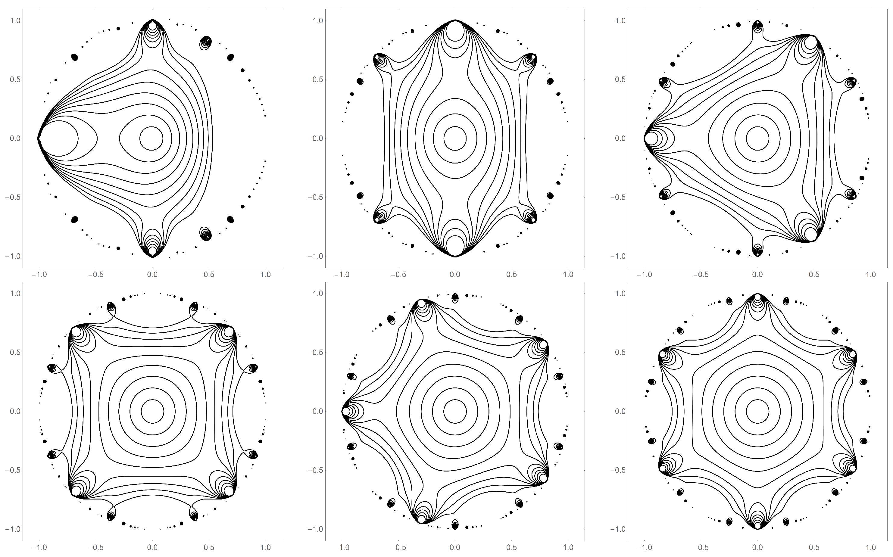
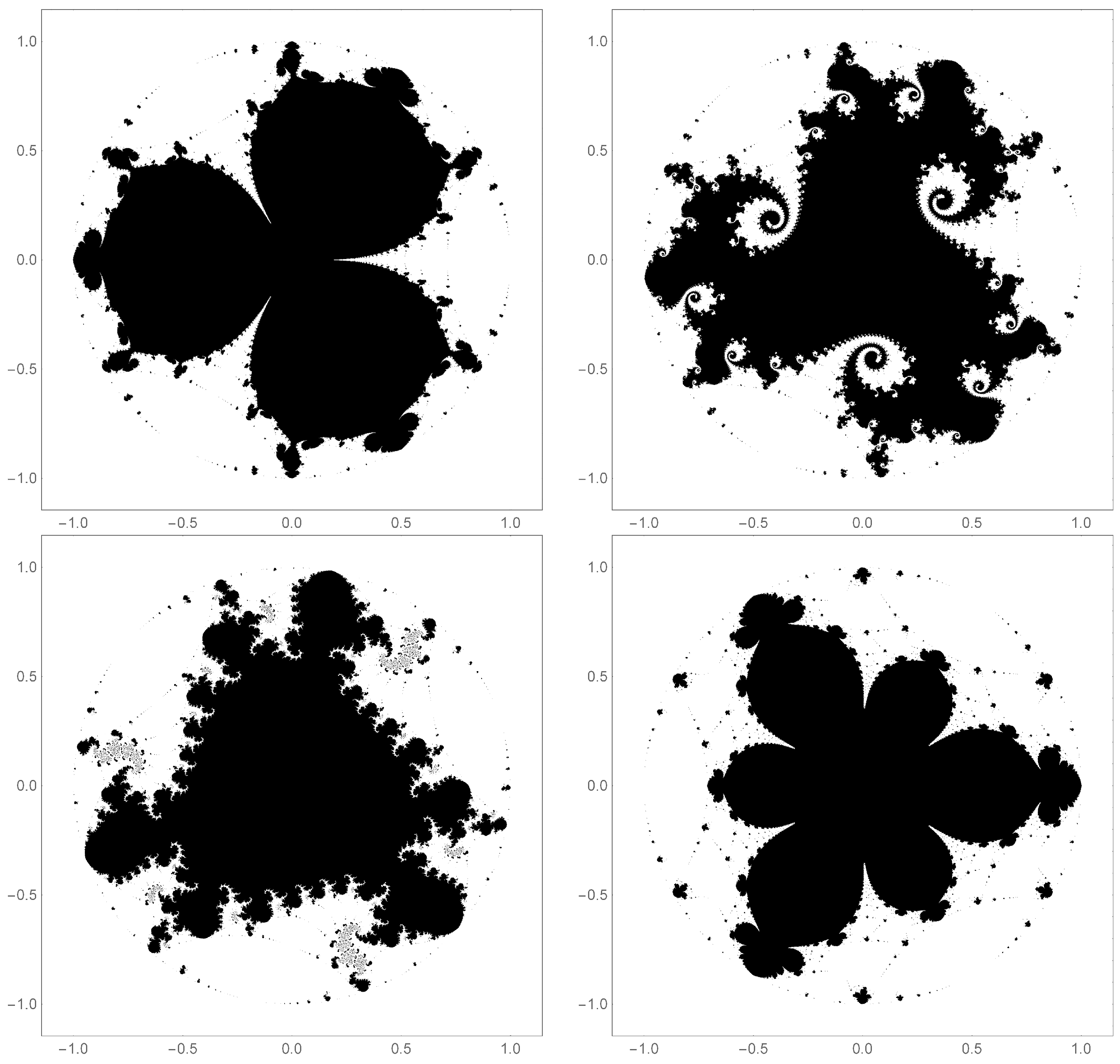
Figure 1.
Contour plots of for value of k 1–6. The contour plots are truncated at the unity level set (). The most prominent feature of a given graph constitutes a subset , which is path-connected to the origin. The complicated nature of produces a host of additional subsets, , that are not path-connected to the origin. These appear adjacent to the natural boundary.
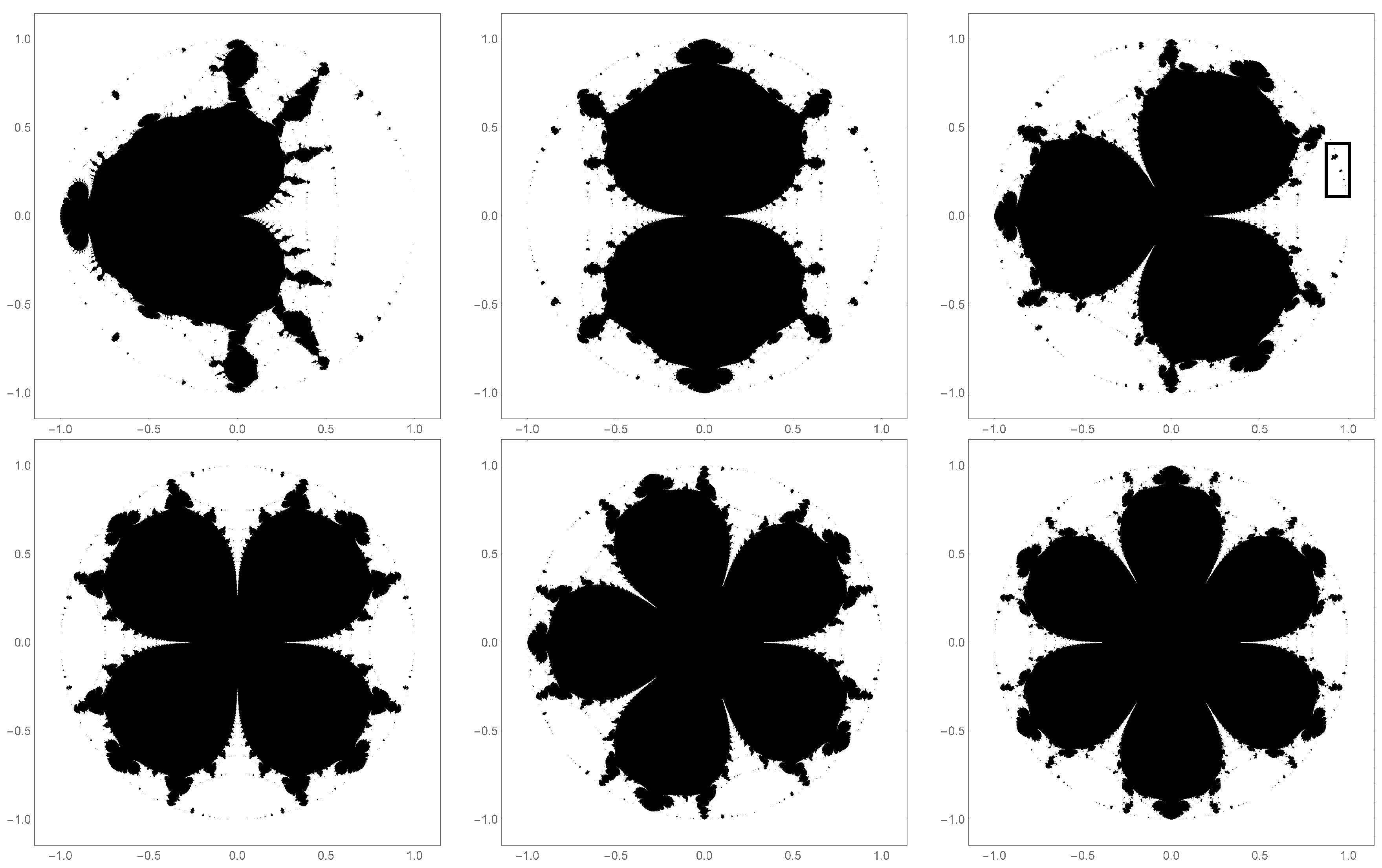
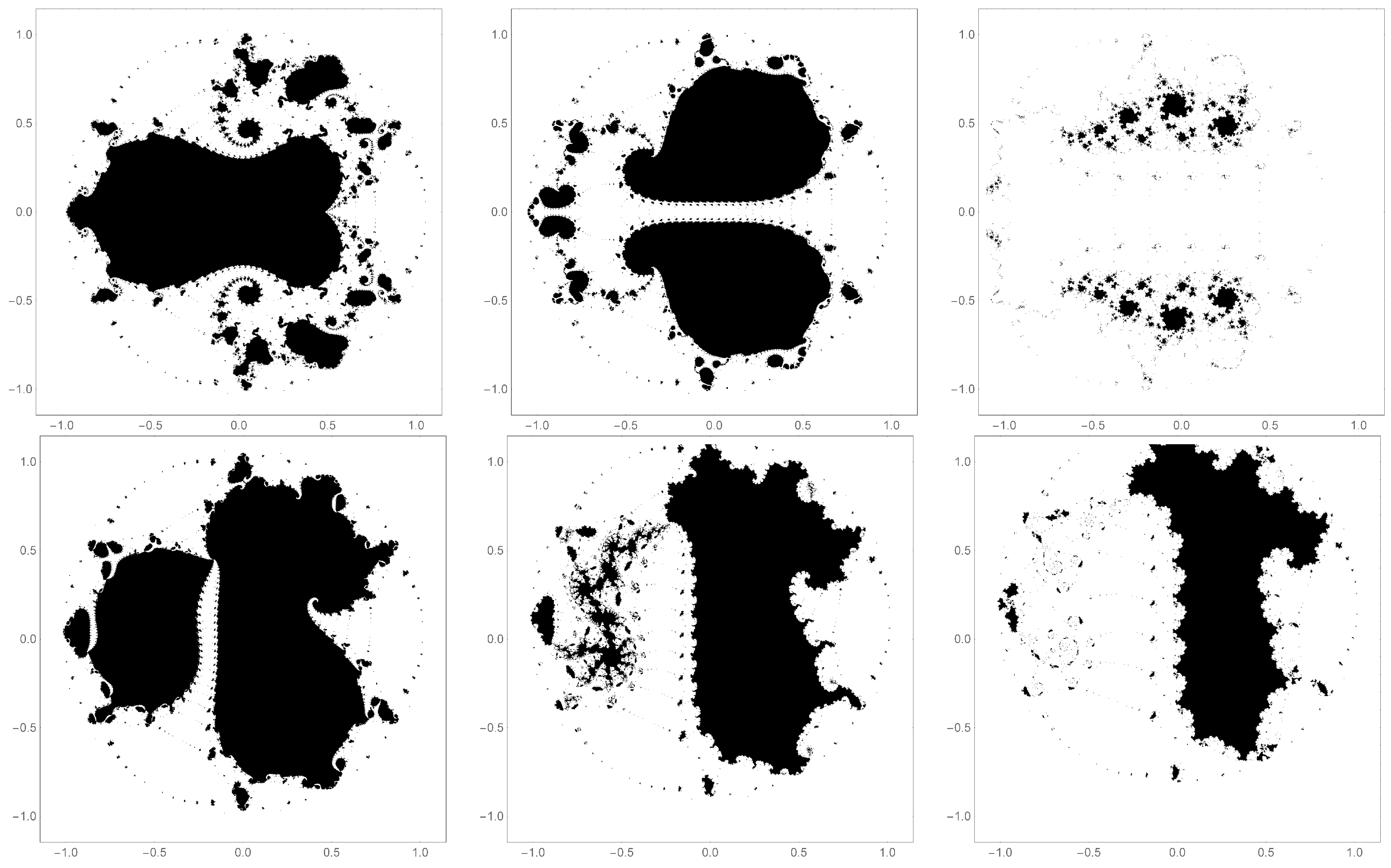
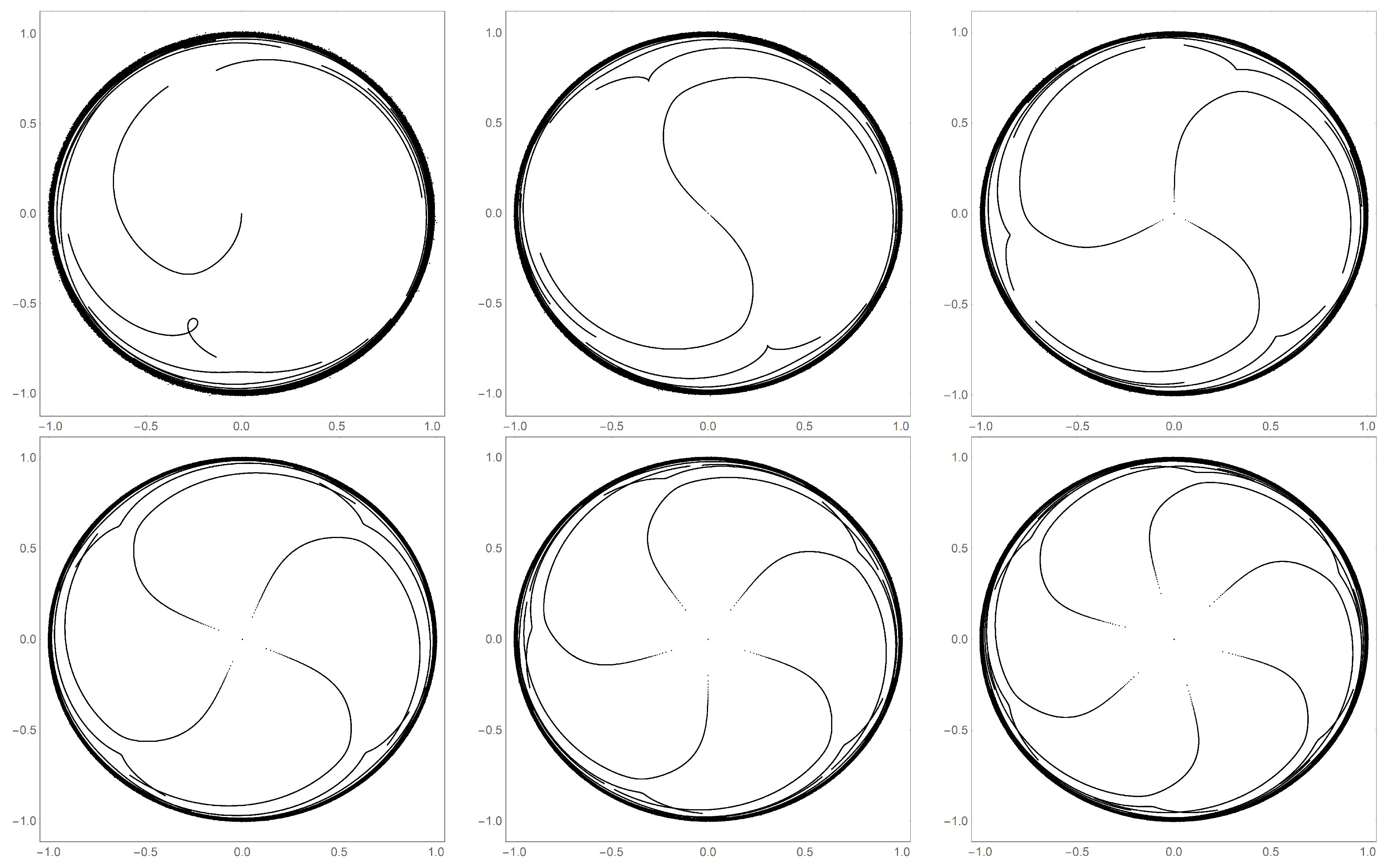
Figure 2.
Base filled-in Julia sets created from the centered polygonal lacunary functions
through
. These filled-in Julia sets arise from the corresponding lacunary functions seen in
Figure 1 for
and
. Notably, they exhibit the same
k-fold symmetry as their corresponding lacunary functions. The points in black represents those points that converge to zero, whereas the white points diverge towards infinity. The principle subset of the filled-in Julia set contains the origin. The subsets not path-connected to the origin are called “islands” (when large) and “islets” (when small). A chain of islands or islets is referred to as an archipelago. (For example, the archipelago in the black box on the upper right graph).
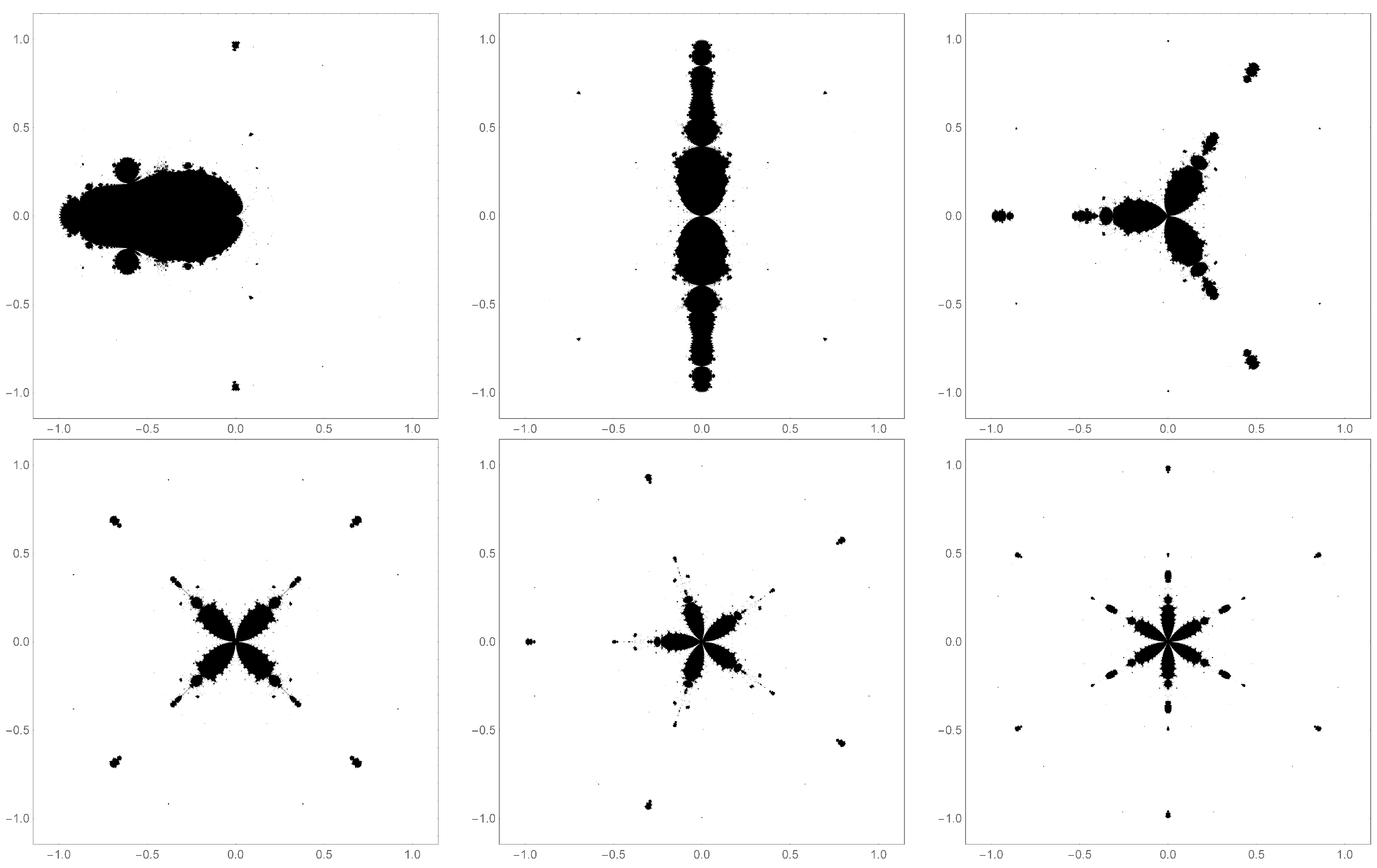
Figure 3.
Mandelbrot sets associated with the corresponding lacunary functions (
Figure 1 and Julia sets (
Figure 2)
through
. From top left to bottom right the Hausdorff modified dimension (described in detail in a later section) of the Mandelbrot sets are 1.363, 1.302, 1.300, 1.335, 1.307, 1.261, 1.321 and 1.247 respectively.
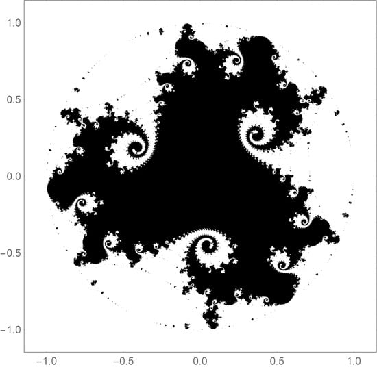
Figure 4.
The filled-in Julia set for . The top left shows the filled-in Julia set for . The top right shows that same filled-in Julia set with a phase rotation, . The bottom left shows the Julia set with a phase rotation. And finally the bottom right shows the Julia set with a phase rotation. Note that phase rotation breaks mirror symmetry but maintains k-fold rotational symmetry.
Figure 5.
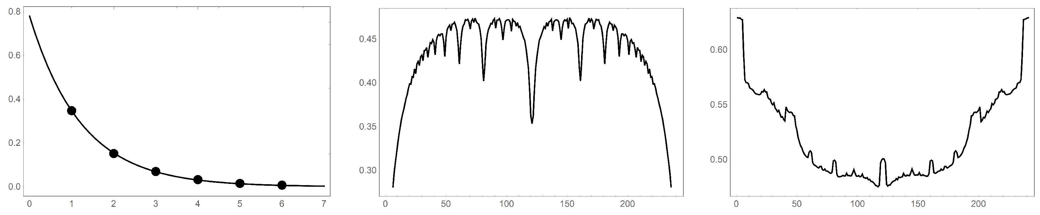
Radius of the Julia set for of the sequence versus j is shown on the left. The radii are plotted along the ordinate and the abscissa is x, where . The data are fit to an exponential decay (fit values: , ). These data expose the very slow ( penetration of the cleft structures in the base filled-in Julia sets (, ). Plots of radius, in the middle and the area as a percentage of the unit disk, on the right, of the Julia sets, as ranges from to . The sharp downward peaks of the middle graph correspond to values where the spirals uncurl to stretch toward the origin. The area graph on the left shows that, although the graphs are not mirrored about the midpoint, the area of these graphs are similar.
Figure 5.
Radius of the Julia set for of the sequence versus j is shown on the left. The radii are plotted along the ordinate and the abscissa is x, where . The data are fit to an exponential decay (fit values: , ). These data expose the very slow ( penetration of the cleft structures in the base filled-in Julia sets (, ). Plots of radius, in the middle and the area as a percentage of the unit disk, on the right, of the Julia sets, as ranges from to . The sharp downward peaks of the middle graph correspond to values where the spirals uncurl to stretch toward the origin. The area graph on the left shows that, although the graphs are not mirrored about the midpoint, the area of these graphs are similar.
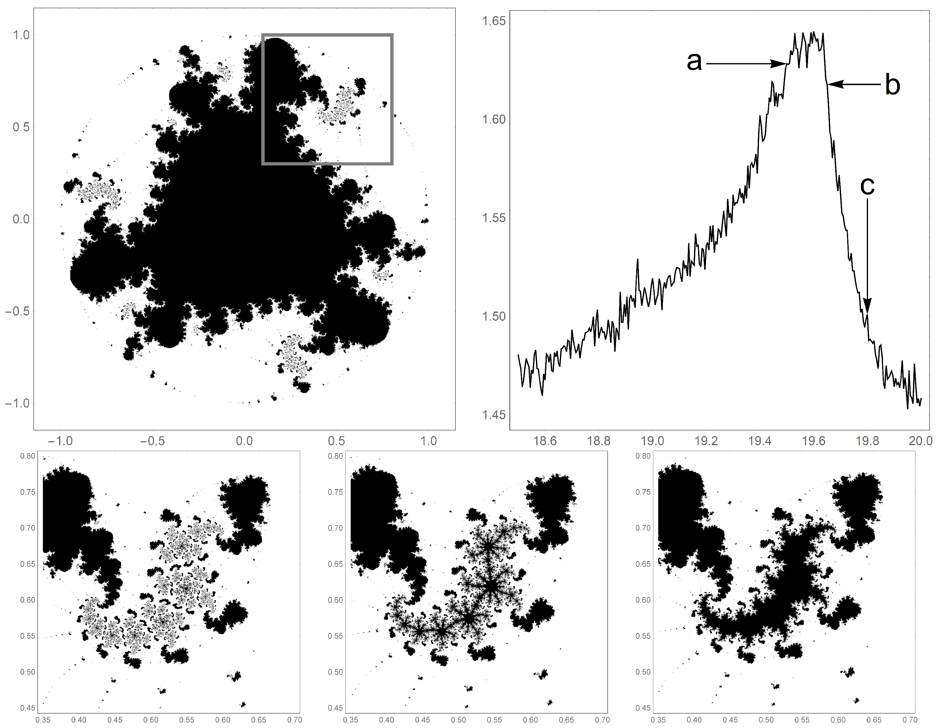
Figure 6.
On the top left is shown the full filled-in Julia set for centered polygonal lacunary function with several islands shown in the box. On the top right is shown a graph of the dimension of the region in the box as the phase is ranging from to . On the bottom left is shown island in the box with a denoted a, phase rotation. In the center of the bottom is shown that same island with a , denoted b, phase rotation. On the bottom right is shown the island with a , denoted c, phase rotation. These bottom images have their dimension shown on the top right graph.
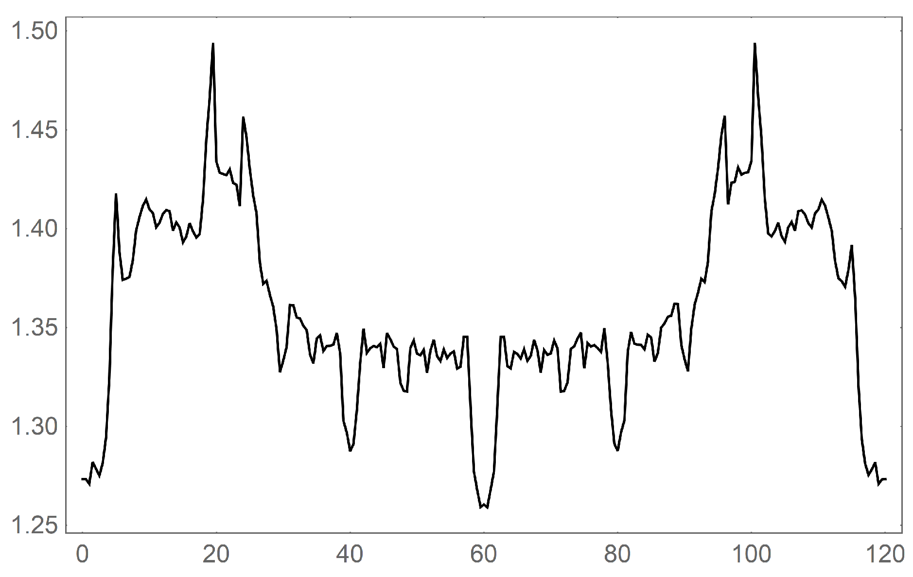
Figure 7.
The plot of dimension for versus phase rotation to . This was calculated using the modified Hausdorff dimension procedure.
Figure 7.
The plot of dimension for versus phase rotation to . This was calculated using the modified Hausdorff dimension procedure.
Figure 8.
Filled-in Julia sets of after an offset parameter has been applied to them. An offset of , 0.04 and 0.20 (top left, center and right respectively) is applied the base filled-in Julia set along the real abscissa. The bottom row shows an offset of , , (left, center and right respectively) along the imaginary ordinate. These offset, filled-in Julia sets make up the corresponding Mandelbrot set. The graphs above were constructed using and with a resolution of 1.5 million pixels.
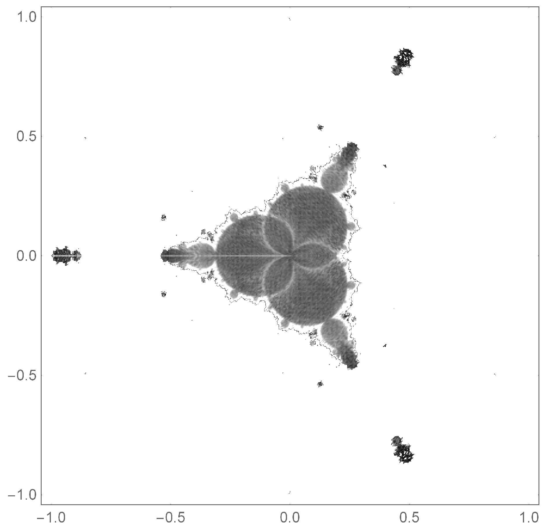
Figure 9.
The calculated box dimension of the Julia sets for 400 by 400 lattice points in the window shown. Typical, the values of the dimension (when calculable) range from approximately 1.1 to 1.8. Low values are dark, high values are light and the white background field are areas where the Julia set is too weak to determine a dimension. It is believed that the 3-fold symmetry holds and thus the light line along the negative real axis is an artifact of the way the lattice points aligned with the Julia set itself. Further, the black outline surrounding the main body is believed to be an artifact as well. This is due to the numerical instability of the dimension calculations for these very weak Julia sets.
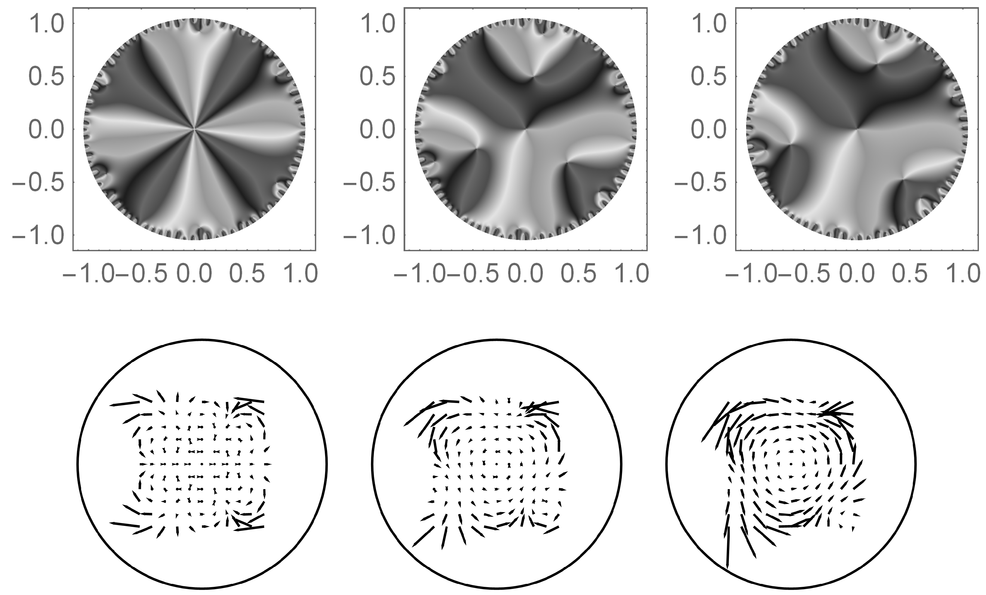
Figure 10.
Two separate representations of the vectors fields for the discrete iterative map The gray-scale representation (top) uses different shades to show which direction arrows are pointing. The vector arrow representation (bottom) uses arrows to show the direction a point moves under one iteration of the map. The phase rotation is for for the left column, for the middle column and for the right column. One notices the emergence of 3 primary fixed points (see text), when . These fixed points move towards the natural boundary as increases.
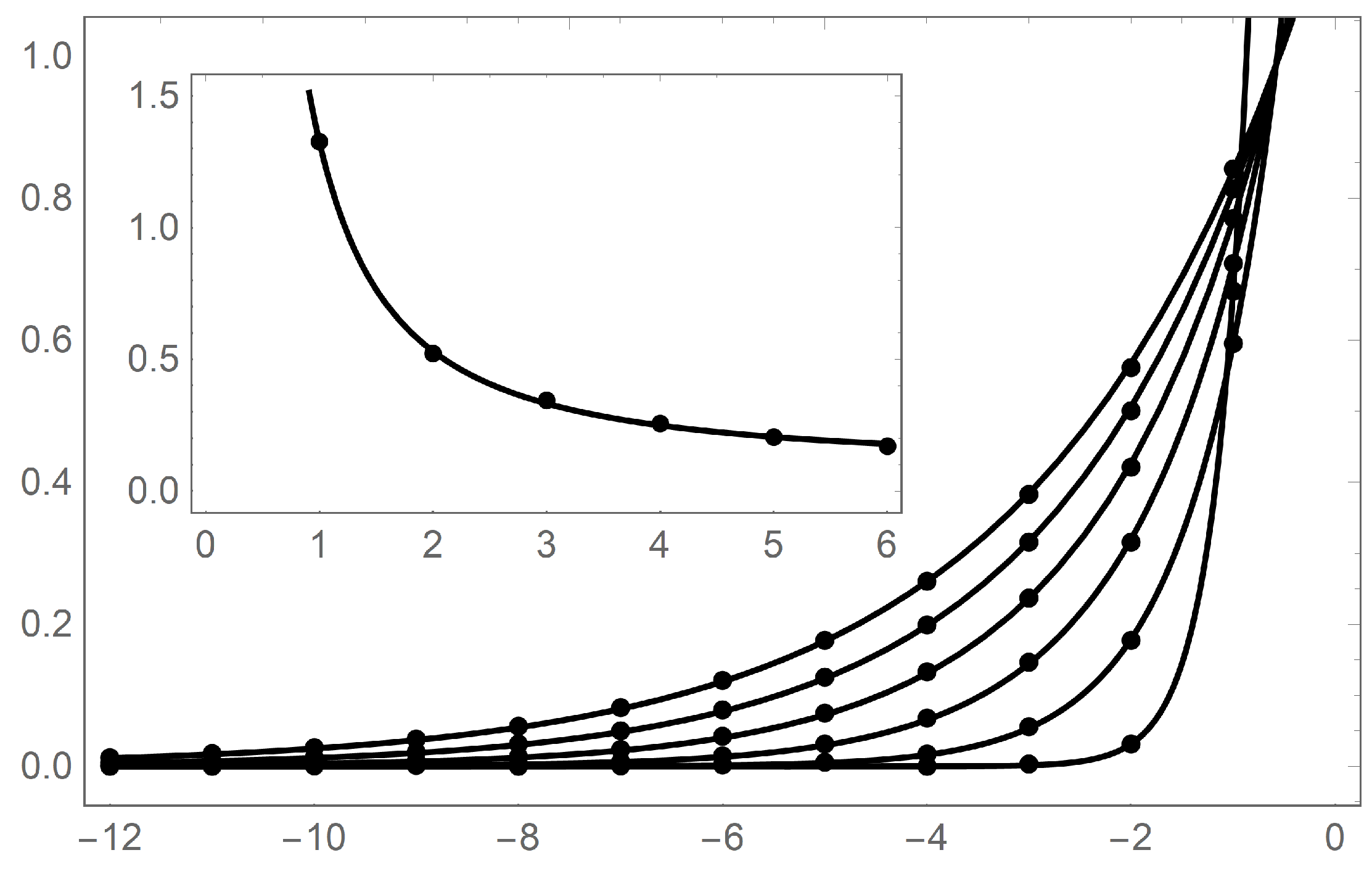
Figure 11.
The primary plot is the radial distance of the fixed points as a function of . Pictured are six exponential line plots corresponding to k values 1–6, with being the right most curve. The value of k increase as the curves sequentially move leftward. The ordinate displays the distance from the origin the fixed point is located (assigned variable d). The abscissa displays . The points on the primary plot can be fit with the function . The inset plot displays the exponent fit parameter a (ordinate) as a function of k (abscissa). These points are fit with a line from the equation . Primary plot fit parameters : , , , , , .
Figure 12.
The movement of the fixed points as runs from to for k values 1–6, . The points originating close to the center are the primary fixed points, whereas the points very close to the unit circle are the secondary fixed points.
Figure 12.
The movement of the fixed points as runs from to for k values 1–6, . The points originating close to the center are the primary fixed points, whereas the points very close to the unit circle are the secondary fixed points.
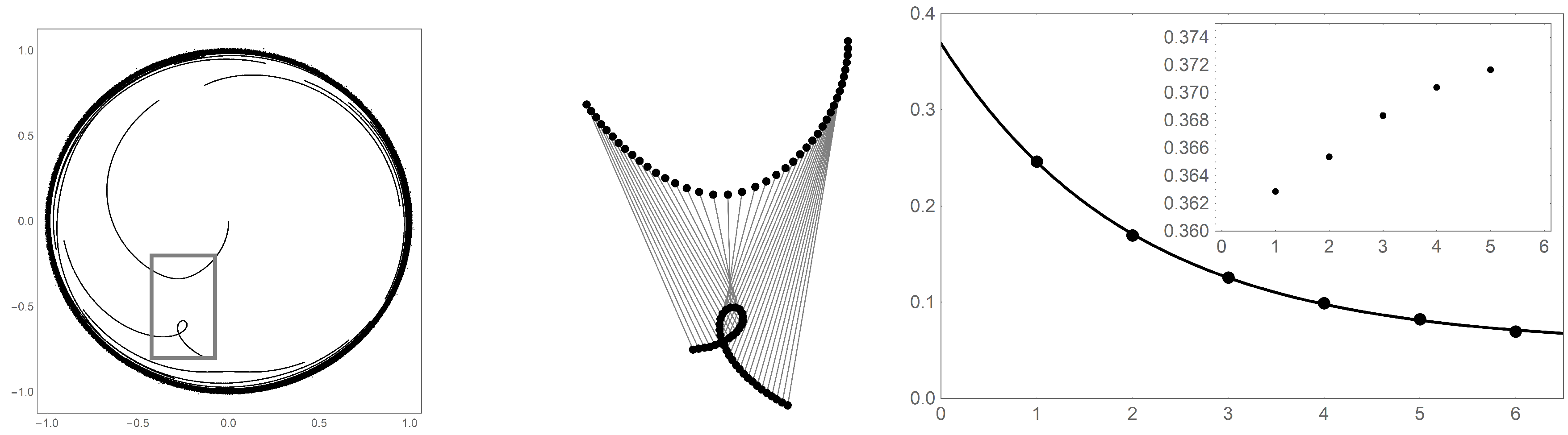
Figure 13.
The path of the primary and secondary fixed points as
increases (left). The middle panel is a blow up of the boxed area of the left graph. The gray tie-lines show the distance between this primary fixed point and this secondary fixed point for a given
value. The minimum distance decreases with
k and seen in the right graph of
Figure 13 (abscissa: k, ordinate: distance). Interestingly the
value that gives the minimum
, is a very weak function of
k, as shown in the inset plot (abscissa:
k, ordinate:
).
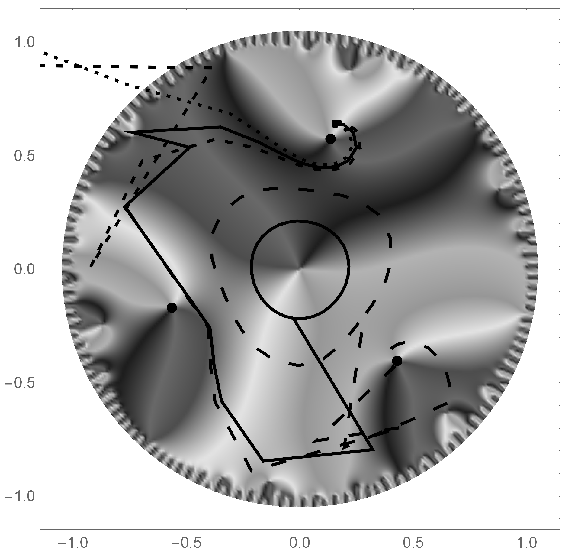
Figure 14.
Iterative trajectories for several nearby initial points for the case of and . The solid line is for the initial point , and 500 iterative steps (the stable orbit is reached after approximately 50 steps). The small and medium sized dashed lines show the trajectories for and respectively. Both of these trajectories exit the unit disk and diverge after 14 and 16 steps respectively. The large dashed line is again for but now (still 500 iterative steps). A different stable orbit is reached after approximately 70 steps and after an excursion to the area near the lower right primary fixed point.
Table 1.
The ratio of an islet’s area to an identified islet’s area for multiple k values when and . For , only four islets are present, whereas for the other k values there are five islets present. The table had an average standard deviation of 0.08205 between the data. This average standard deviation was found by averaging the standard deviation found for each row of data.
| Islet Area Ratios |
|---|
| | | | | | | | |
| 1 to 2 | 1.411 | 1.772 | 1.811 | 1.821 | 1.810 | 1.761 | 1.725 |
| 2 to 3 | 1.326 | 1.378 | 1.386 | 1.383 | 1.373 | 1.366 | 1.362 |
| 3 to 4 | 1.495 | 1.322 | 1.326 | 1.320 | 1.315 | 1.311 | 1.312 |
| 4 to 5 | | 1.507 | 1.511 | 1.508 | 1.504 | 1.810 | 1.503 |
Table 2.
The ratio of an islet’s area to an identified islet’s area for multiple k values when and . The table had an average standard deviation of 0.02027 between the data. This average standard deviation was found by averaging the standard deviation found for each row of data.
Table 2.
The ratio of an islet’s area to an identified islet’s area for multiple k values when and . The table had an average standard deviation of 0.02027 between the data. This average standard deviation was found by averaging the standard deviation found for each row of data.
| Islet Area Ratios |
|---|
| | | | | | | | |
| 1 to 2 | 1.780 | 1.787 | 1.788 | 1.815 | 1.795 | 1.767 | 1.725 |
| 2 to 3 | 1.350 | 1.375 | 1.381 | 1.380 | 1.374 | 1.367 | 1.361 |
| 3 to 4 | 1.280 | 1.314 | 1.321 | 1.317 | 1.315 | 1.306 | 1.311 |
| 4 to 5 | 1.441 | 1.499 | 1.514 | 1.481 | 1.504 | 1.502 | 1.502 |
| 5 to 6 | 0.925 | 0.988 | 0.994 | 1.020 | 0.999 | 0.958 | 1.000 |
Table 3.
The dimension of each of the islets when and . Again, only had four islets while the rest of the k values had 5 islets. The modified Hausdorff dimension was used to find the dimension of these islets.
Table 3.
The dimension of each of the islets when and . Again, only had four islets while the rest of the k values had 5 islets. The modified Hausdorff dimension was used to find the dimension of these islets.
| Islet Dimensions |
|---|
| | | | | | | | |
| Julia set | 1.327 | 1.268 | 1.277 | 1.254 | 1.277 | 1.321 | 1.276 |
| 1 | 1.350 | 1.297 | 1.316 | 1.278 | 1.296 | 1.343 | 1.283 |
| 2 | 1.345 | 1.300 | 1.314 | 1.274 | 1.297 | 1.323 | 1.310 |
| 3 | 1.328 | 1.298 | 1.283 | 1.263 | 1.288 | 1.339 | 1.303 |
| 4 | 1.344 | 1.282 | 1.304 | 1.253 | 1.288 | 1.347 | 1.296 |
| 5 | | 1.273 | 1.296 | 1.281 | 1.286 | 1.333 | 1.302 |
Table 4.
The dimension of each of the islets when and . The modified Hausdorff dimension was used to find the dimension of these islets.
Table 4.
The dimension of each of the islets when and . The modified Hausdorff dimension was used to find the dimension of these islets.
| Islet Dimension |
|---|
| | | | | | | | |
| Julia set | 1.415 | 1.419 | 1.420 | 1.419 | 1.410 | 1.424 | 1.415 |
| 1 | 1.483 | 1.457 | 1.446 | 1.440 | 1.462 | 1.455 | 1.532 |
| 2 | 1.483 | 1.442 | 1.442 | 1.433 | 1.522 | 1.451 | 1.517 |
| 3 | 1.480 | 1.440 | 1.441 | 1.438 | 1.423 | 1.452 | 1.442 |
| 4 | 1.480 | 1.425 | 1.432 | 1.390 | 1.518 | 1.459 | 1.436 |
| 5 | 1.478 | 1.413 | 1.445 | 1.438 | 1.421 | 1.451 | 1.437 |
| 6 | 1.471 | 1.419 | 1.428 | 1.408 | 1.443 | 1.432 | 1.427 |


