Cornu Spirals and the Triangular Lacunary Trigonometric System

Abstract

This work is intended to directly supplement the previous work by Coutsias and Kazarinoff on the foundational understanding of lacunary trigonometric systems and their relation to the Fresnel integrals, specifically the Cornu spirals [Physica 26D (1987) 295]. These systems are intimately related to incomplete Gaussian summations. The current work provides a focused look at the specific system built off of the triangular numbers. The special cyclic character of the triangular numbers modulo m carries through to triangular lacunary trigonometric systems. Specifically, this work characterizes the families of Cornu spirals arising from triangular lacunary trigonometric systems. Special features such as self-similarity, isometry, and symmetry are presented and discussed.

1. Introduction

With the current work, the authors seek to connect with and augment a very interesting study by Coutsias and Kazarinoff, which was published in 1987 [1]. Those authors looked at the lacunary trigonometric system characterized by the sequence, $\mathcal{S}$, of partial summations.

$$\mathcal{S}\equiv \left\{S_N={\displaystyle \sum _{k=0}^N}{e}^{i\pi (\alpha k^r+\beta k)}\right\}$$

(1)

This sequence of partial summations gives rise to a beautiful family of Cornu spirals [1]. These partial summations are a generalization of incomplete Gaussian summations [2,3,4,5,6,7].

Coutsias and Kazarinoff’s work was quite thorough, with a variety of $\alpha$ and r values explored. Quadratic systems ($r=2$) are the most studied in the literature and are intimately connected to basic number theory, specifically in connection with the theta functions studied by Hardy [8,9]. While Coutsias and Kazarinoff discussed the quadratic case, their focus was on the non-quadratic case because of its relative novelty [1]. Furthermore, for the systems described by definition (1), the Cornu spiral patterns arise from choosing irrational values for $\alpha$ ($\beta$ was set to zero in all the data sets discussed) under both the $r=2$ and $r\ne 2$ cases.

The current work takes a slightly modified approach by considering the set of partial summations arising from triangular lacunary trigonometric system,

$${\mathcal{F}}_{n,q}\equiv \left\{f_{n,q}^{\left(N\right)}={\displaystyle \sum _{k=0}^N}{e}^{\frac{i\pi qT\left(k\right)}{n}}\right\},$$

(2)

where $T\left(k\right)\equiv \frac{k(k+1)}{2}$ is the $k^{\mathrm{th}}$ triangular number [10]. ${\mathcal{F}}_{n,q}$ is certainly related to $\mathcal{S}$ and to incomplete Gaussian summations [2], however, there is a critical difference in that the periodic nature of $e^{ix}$ and the presence of the divisor n effectively performs the modulo $2n$ on triangular numbers. The triangular numbers have a very interesting feature in that they are $2m$-periodic under any modulo m (this is discussed further below.) Consequently, the partial summations in ${\mathcal{F}}_{n,q}$ are $4n$-periodic [2,4].

On the one hand, the triangular lacunary system is less general then the one studied by Coutsias and Kazarinoff, but on the other hand, its periodic nature offers an interesting generalization to that work.

Although all of the numerical calculations for this work were a direct summation of the lacunary sequence members by Mathematica, some recent work by Yamada and Ikeda has investigated the use of Padé approximate methods for speeding up the convergence of summations for lacunary functions [11,12].

2. Properties of Triangular Numbers

The set of triangular numbers (also called triangle numbers) has been the subject of a long history of study [10,13], of which major insight has been provided by Gauss himself [14]. In spite of this, it is the observation of the current authors that there is a dearth of literature focused on the triangular numbers mod m, where $m\in {\mathbb{N}}^{+}$ [15].

Of particular importance for the current work is the consideration of the triangle numbers modulo m. The most important aspect of the structure of these numbers is their cyclic nature. It can be proven that the triangular numbers modulo m form a $2m$-cycle for any m and the sequence is symmetric about the “midpoint” of the $2m$-cycle [16]. That is, the last m elements are the reverse sequence to that of the first m elements. It can be shown that this behavior of the triangle numbers modulo m leads to the fact that for each element which appears in ${\mathcal{F}}_{n,q}$, its additive inverse also appears. Thus the sum of the elements of ${\mathcal{F}}_{n,q}$ is zero [16].

As a first example, consider ${\mathcal{F}}_{1,1}$. Here,

$$f_{1,1}^{\left(N\right)}={\displaystyle \sum _{k=0}^N}{e}^{i\pi T\left(k\right)}.$$

(3)

It is immediately seen that one need only consider the triangular numbers modulo 2 (from $n=1$ and $m=2n$), $\left\{0,1,1,0\right\}$, to determine that ${\mathcal{F}}_{1,1}=\left\{1,0,-1,0\right\}$. $f_{1,1}^{(\infty )}$ itself is the divergent series, $f_{1,1}^{(\infty )}=1+0-1+0+1+0-1\dots$.

As a second example consider ${\mathcal{F}}_{2,1}$. Here the set of triangular numbers modulo 4 is $\left\{0,1,3,2,2,3,1,0\right\}$ and leads to ${\mathcal{F}}_{2,1}=\left\{1,1+i,1,0,-1,-1-i,-1,0\right\}$.

3. Lacunary Sequences

An interesting class of mathematical functions are those whose singularities (points of infinity) accumulate along the defined edge of the domain. This is called a natural boundary. One category of such functions are the lacunary (or also called “gap”) functions [17,18]. Lacunary functions are characterized by a Taylor series that has “gaps” (or “lacunae”) in the progression of powers. A prototype example is $f\left(z\right)={\sum }_{n=1}^{\infty }{z}^{n^2}=z+z^4+z^9+z^{16}+\cdots$. The gap theorem of Hadamard [18] says that if the gaps in the powers increase such that the gap tends to infinity as $n\to \infty$, then the function will exhibit a natural boundary. The natural boundary in this example is the unit circle, $\left|z\right|=1$.

Although not heavily used, lacunary functions have been employed in approaches to physical problems. Creagh and White showed that natural boundaries can be important when calculating properties of light outside of elliptic dielectrics [19]. Shado and Ikeda have demonstrated that natural boundaries impact quantum tunneling in some systems [20]. Additionally, Yamada and Ikeda have investigated wavefunctions associated with Anderson-localized states in the Harper model in quantum mechanics [11].

In addition to physics, lacunary functions have found utility in probability theory. Certain lacunary trigonometric systems behave like independent random variables. Most notably they are consistent with the central limit theorem [21]. Lacunary trigonometric functions appear in the context of the random Fourier series in harmonic analysis. Additionally, lacunary functions exhibit features upon approaching the natural boundary that are related to Weiner (stochastic) processes [22].

The $N^{\mathrm{th}}$ member of the lacunary sequence is given by the partial summation,

$$f_N\left(z\right)={\displaystyle \sum _{n=0}^N}{z}^{g\left(n\right)},$$

(4)

where $g\left(n\right)$ is a function of n satisfying the conditions of Hadamard’s gap theorem [18]. To recover a trigonometric lacunary system like the ones studied here and by Coutsias and Kazarinoff, one sets $z=e^{\theta }$. That is, one considers the system at the natural boundary (on the unit circle). All in all, one considers the sequences of finite summations and because of the properties of the triangular numbers modulo m which were listed above, the sequence is cyclic. Consequently, for the triangular lacunary trigonometric systems considered here, one deals with a finite sequence of size $4n$.

4. Fresnel Integrals and the Cornu Spiral

The Fresnel integrals most notably arise from the theory of Fresnel diffraction, which deals with the case where the light source and observer are at a finite distance from the diffraction event [23,24]. They also occur in connection to Greens functions for steady waves [25].

Specifically, the Fresnel integrals are defined via an integral as [26],

$$C\left(t\right)={\int }_0^t\cos \left(\frac{1}{2}\pi x^2\right)dx,S\left(t\right)={\int }_0^t\sin \left(\frac{1}{2}\pi x^2\right)dx.$$

(5)

These functions are also represented as a series [26],

$$\begin{array}{cc}C\left(t\right)& ={\displaystyle \sum _{n=0}^{\infty }}\frac{{(-1)}^n{\left(\frac{1}{2}\pi \right)}^{2n}}{\left(2n\right)!(4n+1)}{z}^{4n+1},\end{array}$$

(6)

$$\begin{array}{cc}S\left(t\right)& ={\displaystyle \sum _{n=0}^{\infty }}\frac{{(-1)}^n{\left(\frac{1}{2}\pi \right)}^{2n+1}}{(2n+1)!(4n+3)}{z}^{4n+3}.\end{array}$$

(7)

As a consequence of the Euler identity,

$$C\left(t\right)+iS\left(t\right)={\int }_0^t{e}^{\frac{1}{2}i\pi x^2}dx.$$

(8)

Finally, the Fresnel integrals can be cast in terms of the confluent hypergeometric function, ${}_1{F}_1$,

$$C\left(z\right)+iS\left(z\right)=z{}_1{F}_1\left(\frac{1}{2},\frac{3}{2},\frac{\pi i{z}^2}{2}\right)$$

(9)

One useful way to represent the Fresnel integrals is to parametrically plot $C\left(t\right)$ versus $S\left(t\right)$. This gives rise to the well-known Cornu spiral. In addition to its use in optics, the Cornu spiral has also found use in highway design [27], Kloosterman paths [28], and Van der Corput transforms [29]. Very recently Milici et al. [30] have studied fractional Cornu spirals via the machinery of fractional calculus.

More pertinent to the current work, Lehmer showed that Cornu spirals arise from incomplete Gaussian summations [2], which encompass the triangular lacunary trigonometric system of the current work. Berry and Goldberg developed a renormalization procedure for such Cornu spirals [4] as did Sinai [31] and Fedotov and Klopp [32], while Cellarosi and Marklof investigated the related quadratic Weyl summations [33], and Paris provided much insight into various expansions of such systems along with asymptotic behavior [3]. Indeed families of, at times elaborate, combinations of Cornu spirals arise when considering ${\mathcal{F}}_{n,q}$.

5. Results and Discussion

For large values of n, the points in the sequence ${\mathcal{F}}_{n,1}$ trend towards lying along the Cornu spiral parameterized by,

$$S{p}_{n,1}=\left(\sqrt{n}C\left(t\right),\sqrt{n}S\left(t\right)\right).$$

(10)

This spiral has $C_2$ rotational symmetry (equivalent to inversion symmetry in the plane) about the origin. Thus, $Sp$ has its inflection point at the origin. The spiral centers are at $\frac{\sqrt{n}}{2}(1+i)$ and $-\frac{\sqrt{n}}{2}(1+i)$.

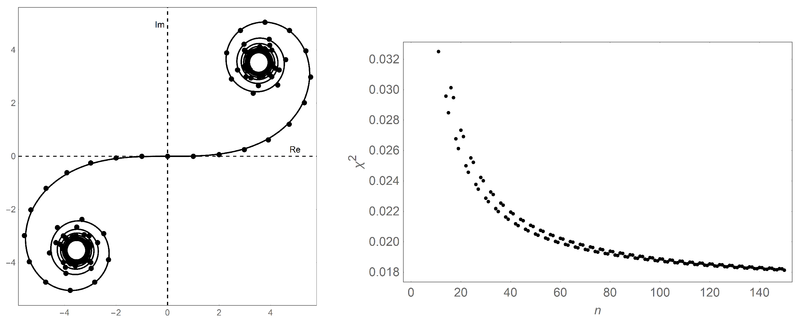
The points of ${\mathcal{F}}_{n,1}$ fall equally spaced along the Cornu spiral and each point occurs twice in the sequence. The spacing between adjacent points is $\frac{1}{2\sqrt{n}}$ and the total arclength of the curve is $\frac{2n+1}{2\sqrt{n}}\simeq \sqrt{n}$ for large n. Changing the value of n only scales the Cornu spiral; it does not change the shape.

The left panel of Figure 1 provides an illustrative example for the case of ${\mathcal{F}}_{50,1}$. Even at only $n=50$, the Cornu spiral models the data very well. $C_2$ rotational symmetry is clear, the spiral centers are seen to be at $\frac{\sqrt{50}}{2}(1+i)$ and $-\frac{\sqrt{50}}{2}(1+i)$, and the inflection point is at the origin. The points from ${\mathcal{F}}_{50,1}$ are evenly spaced along the Cornu spiral with a step size of $\frac{1}{2\sqrt{50}}$.

The right panel of Figure 1 shows the ${\chi }^2$ values for n ranging from 1 to 150. Each datum is obtained by evaluating the summation of the squares of the difference between the value of the partial summmation in ${\mathcal{F}}_{n,1}$ and the Cornu spiral itself. This is normalized by the total number of points. A progression, albeit not monotonic, to lower and lower ${\chi }^2$ values is seen.

Increasing the value of q brings about a qualitatively (and somewhat quantitatively) predictable change in the general shape of the spiral patterns. These spirals will be referred to here as higher order Cornu spirals as they consist of linked Cornu spiral “monomer units”.

The general features of the ${\mathcal{F}}_{n,q}$ sequences are as follows. If q does not share a common divisor with n, then the higher order Cornu spirals will consist of q chain-linked Cornu spiral monomers. Every two adjacent monomer Cornu spirals will share a center. Furthermore, the overall $C_2$ symmetry of the higher order Cornu spiral is maintained.

The base monomer Cornu spiral is parameterized as,

$$S{p}_{n,q}=\sqrt{\frac{n}{q}}\left(C\left(t\right),S\left(t\right)\right).$$

(11)

The other monomer Cornu spirals in the chain are obtained through the isometric transformation of the base monomer.

If q shares a common divisor with n, then the fraction $\frac{q}{n}$ reduces to $\frac{p}{m}$. Consequently, one simply considers ${\mathcal{F}}_{m,p}$.

It is interesting to explore the case of holding q constant and changing n. In this case, the higher order Cornu spiral will sweep through q distinct shapes before repeating the pattern. It is obvious that if q is prime, there will be one member of this set of higher order Cornu spirals that reduces to that of ${\mathcal{F}}_{m,1}$. And if q is composite, there will be several reduced shapes appearing. 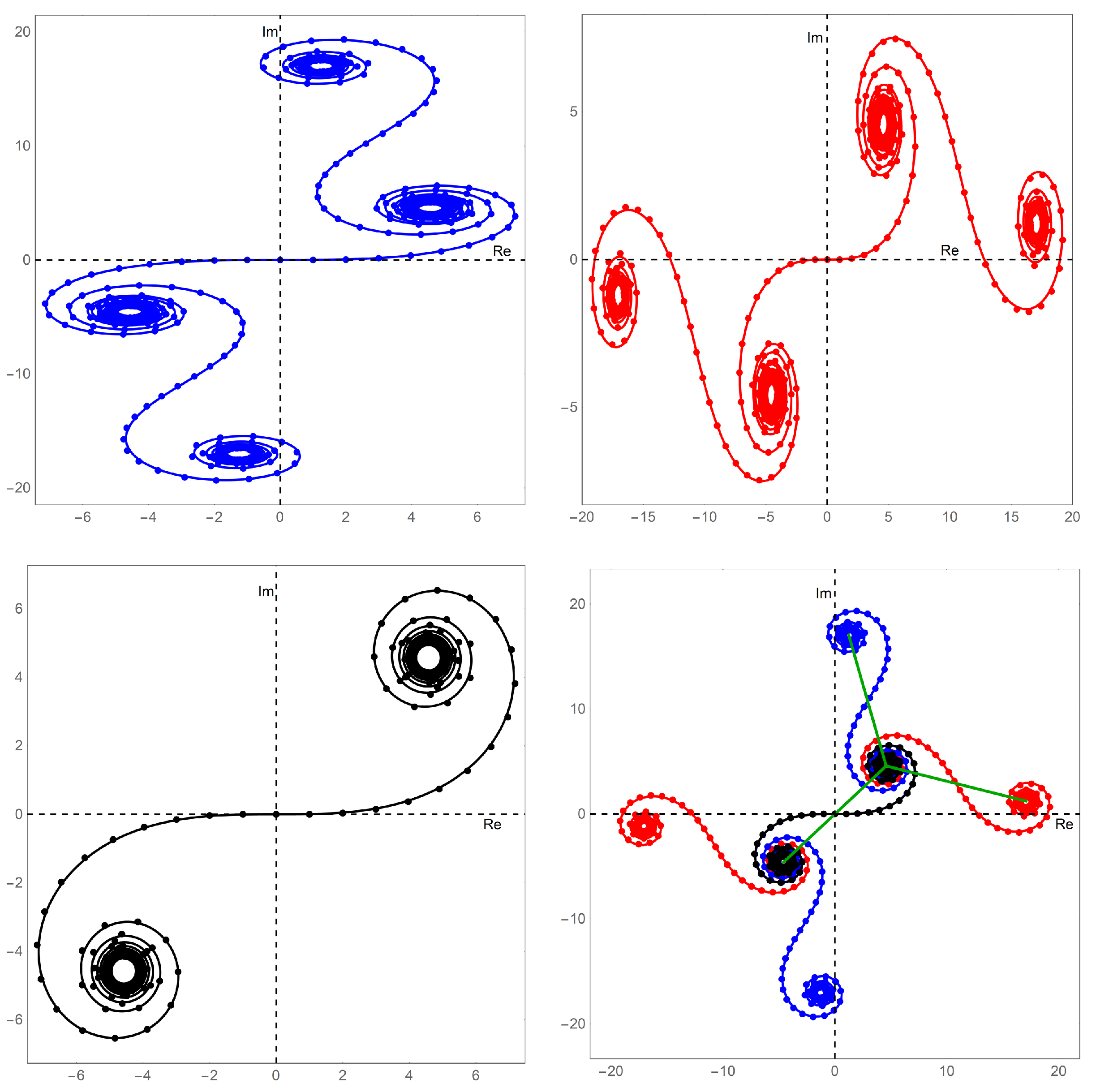Figure 2 and Figure 3 illustrate the above qualitative analysis where Figure 2 collects the set of three generic shapes for $q=3$, while Figure 3 does so for the five generic shapes associated with $q=5$.

5.1. Isometry and Quasi-Symmetry

Each monomer in the higher order Cornu spiral is related to the base monomer (Equation (11)) via an isometric transformation involving only rotation and translation. A given isometry is represented as,

$${\widehat{I}}_{\varphi ,z_0}Sp=\sqrt{\frac{n}{q}}\left(\cos \left(\varphi \right)C\left(t\right)-\sin \left(\varphi \right)S\left(t\right)+x_0,\sin \left(\varphi \right)C\left(t\right)+\cos \left(\varphi \right)S\left(t\right)+y_0\right),$$

(12)

where $\varphi \in \mathbb{R}$ and $z_0=x_0+i{y}_0$. The higher order Cornu spiral is then the piecewise collection of all transformed monomers along with the base monomer.

As a concrete example, consider the case of $q=3$ as shown in Figure 2. The two non-reduced shapes in this family are ${\mathcal{F}}_{250,3}$ (left panel) and ${\mathcal{F}}_{251,3}$ (right panel). Consider first ${\mathcal{F}}_{250,3}$. Note that because of the enforced $C_2$ rotational symmetry, one need only determine one of the two isometries. This is because if ${\widehat{I}}_{\varphi ,z_0}$ is an isometry, then so is ${\widehat{I}}_{\varphi ,z_0^{*}}$. Determination of the isometry yields $\varphi =\frac{\pi }{3}$ and

$$z_0=\frac{1}{2}\left(\cos \left(\frac{\pi }{3}\right)-\sin \left(\frac{\pi }{3}\right)+1\right)+\frac{i}{2}\left(\cos \left(\frac{\pi }{3}\right)+\sin \left(\frac{\pi }{3}\right)+1\right).$$

Furthermore, determination of the isometry for ${\mathcal{F}}_{251,3}$ yields $\varphi =-\frac{\pi }{3}$ and

$$z_0=\frac{1}{2}\left(\cos \left(-\frac{\pi }{3}\right)-\sin \left(-\frac{\pi }{3}\right)+1\right)+\frac{i}{2}\left(\cos \left(-\frac{\pi }{3}\right)+\sin \left(-\frac{\pi }{3}\right)+1\right).$$

For general q, the set of isometries is given by $\varphi =j\frac{\pi }{q}$ and

$$z_0=\frac{1}{2}\left(\cos \left(j\frac{\pi }{q}\right)-\sin \left(j\frac{\pi }{q}\right)+1\right)+\frac{i}{2}\left(\cos \left(j\frac{\pi }{q}\right)+\sin \left(j\frac{\pi }{q}\right)+1\right),$$

where j is odd and ranges from $-q$ to q. The isometries required for the $2^{\mathrm{nd}}$ level and higher monomers, although straightforward to determine, become increasingly complicated to explicitly determine. There also seems to be little additional insight gained by doing so.

An interesting quasi-symmetry becomes apparent when viewing the members of a family superimposed in one graph as in the lower right panels of Figure 2 and Figure 3. The centers of the base monomer Cornu spiral serves as the origin for a local q-fold rotational quasi-symmetry. The trifoil and pentifoil placed on the graphs help guide the eye to this quasi-symmetry.

Care is taken to use the modifier “quasi” because n is different for each member of the family. Thus their respective component monomer Cornu spirals are different. This difference reduces to zero as n approaches infinity.

5.2. Series Relations

The triangular lacunary trigonometric function itself ($N\to \infty$) can be can be related to a Jacobi theta function [26]. Writing,

$$f_{n,q}^{\left(N\right)}={\displaystyle \sum _{k=0}^N}{e}^{\frac{i\pi qT\left(k\right)}{n}}={\displaystyle \sum _{k=0}^N}{e}^{\frac{i\pi q}{2n}\left(k^2+k\right)}.$$

Then completing the square in the exponent gives,

$$f_{n,q}^{\left(N\right)}={\displaystyle \sum _{k=0}^N}{e}^{\frac{i\pi q}{2n}{\left(k+\frac{1}{2}\right)}^2}{e}^{\frac{i\pi q}{8n}}.$$

Extending the dummy index to $-N$ and dividing by 2 yields,

$$f_{n,q}^{\left(N\right)}=\frac{1}{2}{e}^{\frac{i\pi q}{8n}}{\displaystyle \sum _{k=-N}^N}{e}^{\frac{i\pi q}{2n}{\left(k+\frac{1}{2}\right)}^2}.$$

At this point one considers $\overline{q}\equiv q+iϵ$, where $ϵ$ is a small positive real number. N is then taken to infinity such that,

$$f_{n,\overline{q}}^{(\infty )}=\frac{1}{2}{e}^{\frac{i\pi \overline{q}}{8n}}{\displaystyle \sum _{k=\infty }^{\infty }}{e}^{\frac{i\pi \overline{q}}{2n}{\left(k+\frac{1}{2}\right)}^2},$$

(13)

where the summation is recognized at the second Jacobi theta function [26]. Hence,

$$f_{n,\overline{q}}^{(\infty )}=\frac{1}{2}{e}^{\frac{i\pi q}{8n}}{e}^{\frac{-\pi ϵ}{8n}}{\vartheta }_2\left(0,\frac{1}{2}{e}^{\frac{i\pi q}{2n}}{e}^{\frac{-\pi ϵ}{2n}}\right).$$

(14)

Taking the limit of vanishing $ϵ$ yields,

$$f_{n,q}^{(\infty )}={\displaystyle \underset{ϵ\to 0}{\lim }}\frac{1}{2}{e}^{\frac{i\pi q}{8n}}{e}^{\frac{-\pi ϵ}{8n}}{\vartheta }_2\left(0,\frac{1}{2}{e}^{\frac{i\pi q}{2n}}{e}^{\frac{-\pi ϵ}{2n}}\right).$$

(15)

Now, letting ${\delta }_n\equiv e^{\frac{-\pi ϵ}{2n}}$, one can write,

$$f_{n,q}^{(\infty )}=\frac{1}{2}{e}^{\frac{i\pi q}{8n}}{\displaystyle \underset{{\delta }_n\to 1}{\lim }}{\vartheta }_2\left(0,\frac{1}{2}{\delta }_n{e}^{\frac{i\pi q}{2n}}\right).$$

(16)

Equation (9) along with large n gives rise to an approximate series relation for the members of ${\mathcal{F}}_{n,1}$. Noting that these values appear uniformly along the Cornu spiral at position and using Equation (9),

$$f_{n,1}^{\left(N\right)}\simeq \frac{N}{2}{}_1{F}_1\left(\frac{1}{2},\frac{3}{2},\frac{\pi i{\left(\frac{N}{2\sqrt{n}}\right)}^2}{2}\right).$$

(17)

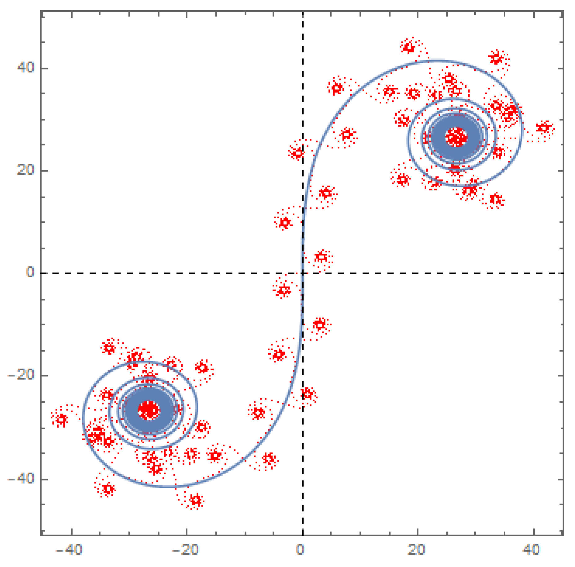
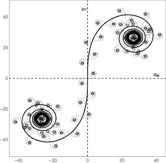
5.3. Large n and Self-Similarity

Lacunary functions in general, and lacunary trigonometric functions in particular, exhibit scaling and self-similarity in many interesting ways. The emergence of the higher order Cornu spirals is no exception. Firstly, it is already clear that the higher order Cornu spirals are made up of identical component Cornu spirals. Secondly, for certain high order Cornu spirals, remarkable self-similarity emerges in which the inflection points of the component monomers fall along a base Cornu spiral themselves. The example of the ${17}^{\mathrm{th}}$ member of the set of curves from ${\mathcal{F}}_{2831,67}$ is shown in Figure 4. Indeed the inflection points of the 67 monomer Cornu curves lie on the base Cornu spiral albeit rotated by $\frac{\pi }{2}$. It is further noted that the component Cornu spiral alternates between lying normal to and tangent to the larger Cornu spiral. Berry and Goldberg [4] and Coutsias and Kazarinoff [1] discuss a similar self-similarity of non-periodic systems. They further discuss the potential for renormalization procedures.

6. Conclusions

This work added to the foundational understanding of lacunary trigonometric systems and their relation to the Fresnel integrals and specifically the Cornu spirals. Such systems are intimately related to incomplete Gaussian summations and a thorough analysis was previously provided by Coutsias and Kazarinoff. The current work supplemented this study and provided a focused look at the specific system built off of the triangular numbers. The special cyclic character of the triangular numbers modulo (any) m carry through to triangular lacunary trigonometric systems.

Specifically, this work characterized the families of Cornu spirals arising from triangular lacunary trigonometric systems. Special features such as self-similarity, isometry, and symmetry were investigated and discussed. It is hoped that this work will provide foundational information that can be used to build upon towards applied problems in physics.