Fractional Mass-Spring-Damper System Described by Generalized Fractional Order Derivatives

Abstract

This paper proposes novel analytical solutions of the mass-spring-damper systems described by certain generalized fractional derivatives. The Liouville–Caputo left generalized fractional derivative and the left generalized fractional derivative were used. The behaviors of the analytical solutions of the mass-spring-damper systems described by the left generalized fractional derivative and the Liouville–Caputo left generalized fractional derivative were represented graphically and the effect of the orders of the fractional derivatives analyzed. We finish by analyzing the global asymptotic stability and the converging-input-converging-state of the unforced mass-damper system, the unforced spring-damper, the spring-damper system, and the mass-damper system.

1. Introduction

Currently, many models in physics [1,2], mechanics [2,3], science and engineering [4], bio-mathematics [5], biology [5], and finance and economics [6,7] can be modeled using fractional derivatives. Fractional calculus has many applications in real-life problems. The recent investigations of the applications of fractional calculus were published in different areas. In [8], the authors modeled the electrical circuits using the fractional derivative operator. In [9], Santos modeled the nonlinear diffusion equations with statistical processes using non-integer derivatives. In finance and economics, Yavuz [7] used the fractional derivative to modeled the Black–Scholes equations. In physics and mathematical methods for physics, Hristov proposed new diffusion equations using the Atangana–Baleanu fractional derivative in [10,11]. Sene proposed the analytical solution of the Stokes first equation [12], fractional diffusion equations [9,13], and Cateneao–Hristov equations [14]. For more recent applications of fractional calculus, see [15,16].

Recently, the modeling of the mass-spring-damper equation using fractional derivatives has interested some authors. In [17], the authors modeled the mass-spring-damper equation using the Liouville–Caputo fractional derivative and the Caputo-Fabrizio fractional derivative. The analytical solution of the fractional mass-spring-damper equation has been proposed and the classical mass-spring-damper equation and the fractional mass-spring damper equation compared. In [18], Ray et al. proposed a new method for getting the analytical solution of the mass-spring-damper equation described by the Riemann–Liouville fractional derivative. In [19], Gómez-Aguilar introduced the mass-spring and damper-spring models in the context of the Liouville–Caputo fractional derivative. He proposed the analytical solutions and the numerical simulations. In [1], Delgado et al. proposed the mass-spring-damper system involving variable order fractional derivatives. The authors in [1] obtained analytical solutions for this system involving variable-order derivatives of the Atangana–Koca type. In [20], the authors considered the fractional mass-spring damper equation and proposed an experimental evaluation of the viscous damping coefficient in the fractional underdamped oscillator. In [4], the authors obtained analytical solutions for the mass-spring damper system involving the Liouville–Caputo fractional derivative and the Laplace transform.

In this paper, we study the mass-spring-damper system with certain fractional generalized derivatives. We consider the Liouville–Caputo generalized fractional derivative and the left generalized fractional derivative. The Laplace transform of the previous operators is used to obtain the analytical solutions of the mass-spring-damper equations in three cases: in the absence of mass, in the absence of a spring, and the mass-spring-damper equation. Furthermore, we will investigate two properties of the introduced models, and we will prove that the fractional mass damper equation described by certain generalized fractional derivatives satisfies the converging-input-converging-state. Furthermore, in the absence of the exogenous input, the trivial solution of the mass damper equation is Mittag–Leffler stable.

The paper is structured as follows: In Section 2, we propose the background on the generalized fractional derivatives. In Section 3, we obtain the analytical solution of the mass-damper equation, the analytical solution of the spring-damper equation, and the analytical solution of the mass-spring-damper equation described by the Liouville–Caputo left generalized fractional derivative. We analyze using the stability notion the behavior of the obtained analytical solutions. In the same section, we obtain analytical solutions for the above cases considering the left generalized fractional derivative. Finally, in Section 4, we finish by giving the concluding remarks.

2. Generalized Fractional Derivative Operators

The generalized fractional derivatives and integrals are the generalized form of the Liouville–Caputo fractional derivative, the Riemann–Liouville fractional derivative, and the Riemann fractional integral. The definition and lemma recalled in this section is the recent advancement in the generalization of the fractional derivative and integral and can be found in [21,22]. For more investigation related to the generalized fractional derivatives, see [21,22,23].

Definition 1.

The generalized integral of order α with $\rho >0$ of a continuous function $g:[a,+\infty [⟶\mathbb{R}$ is defined by the following form:

$$\left(I^{\alpha ,\rho }g\right)\left(t\right)=\frac{1}{\Gamma \left(\alpha \right)}{\int }_a^t{\left(\frac{t^{\rho }-s^{\rho }}{\rho }\right)}^{\alpha -1}g\left(s\right)\frac{ds}{s^{1-\rho }},$$

(1)

where $\Gamma (·)$ denotes the Gamma function, for, i.e., $t>a,$ and $0<\alpha <1$.

Definition 2.

The left generalized fractional derivative of order α with $\rho >0$ of a continuous function $g:[a,+\infty [⟶\mathbb{R}$ is defined by the following form:

$$\left(D^{\alpha ,\rho }g\right)\left(t\right)=\left(I^{1-\alpha ,\rho }g\right)\left(t\right)=\frac{1}{\Gamma (1-\alpha )}\left(t^{1-\rho }\frac{d}{dt}\right){\int }_a^t{\left(\frac{t^{\rho }-s^{\rho }}{\rho }\right)}^{-\alpha }g\left(s\right)\frac{ds}{s^{1-\rho }},$$

(2)

where $\Gamma (·)$ denotes the Gamma function, for, i.e., $t>a,$ and $0<\alpha <1$.

Definition 3.

The Liouville–Caputo generalized fractional derivative of order α with $\rho >0$ of a continuous function $g:[a,+\infty [⟶\mathbb{R}$ is defined by the following expression:

$$\left(D_c^{\alpha ,\rho }g\right)\left(t\right)=\frac{1}{\Gamma (1-\alpha )}{\int }_a^t{\left(\frac{t^{\rho }-s^{\rho }}{\rho }\right)}^{-\alpha }\gamma g\left(s\right)\frac{ds}{s^{1-\rho }},$$

(3)

where $\Gamma (·)$ denotes the Gamma function, for, i.e., $t>a,$ $\gamma =t^{1-\rho }\frac{d}{dt}$ and $0<\alpha <1$.

Definition 4.

The ρ-Laplace transform of the Liouville–Caputo generalized fractional derivative of a continuous function $g:[a,+\infty [⟶\mathbb{R}$ is defined by the following expression:

$${\mathcal{L}}_{\rho }\left\{\left(D_c^{\alpha ,\rho }g\right)\left(t\right)\right\}=s^{\alpha }{\mathcal{L}}_{\rho }\left\{g\left(t\right)\right\}-s^{\alpha -1}g\left(a\right),$$

(4)

where the ρ-Laplace transform of a given function $g:[a,+\infty [⟶\mathbb{R}$ is represented by:

$${\mathcal{L}}_{\rho }\left\{g\left(t\right)\right\}\left(s\right)={\int }_a^{\infty }{e}^{-s\frac{t^{\rho }}{\rho }}g\left(t\right)\frac{dt}{t^{1-\rho }}.$$

(5)

Definition 5.

The ρ-Laplace transform of the left generalized fractional derivative of a function $g:[a,+\infty [⟶\mathbb{R}$ is defined by the following expression:

$${\mathcal{L}}_{\rho }\left\{\left(D^{\alpha ,\rho }g\right)\left(t\right)\right\}=s^{\alpha }{\mathcal{L}}_{\rho }\left\{g\left(t\right)\right\}-\left(I^{1-\alpha ,\rho }g\right)\left(a\right).$$

(6)

Definition 6.

The Mittag–Leffler function with two parameters is defined in the following form:

$$E_{\alpha ,\beta }\left(z\right)=\sum _{k=0}^{\infty }\frac{z^k}{\Gamma (\alpha k+\beta )},$$

(7)

where $\alpha >0,$ $\beta \in \mathbb{R}$ and $z\in \mathbb{C}$. The classical exponential function is recovered when the orders satisfy $\alpha =\beta =1$.

3. Fractional Mass-Spring-Damper Systems

We obtain the analytical solutions for the fractional mass-spring-damper equation described by the generalized fractional derivatives. We consider three cases: the fractional mass-spring damper equation represented by the generalized fractional operators in absence of mass, the fractional mass-spring damper equation described by the generalized fractional operators in the absence of a spring, and finally, the fractional mass-spring damper equation represented by the generalized fractional operators. We study the converging-input-conversing-state and the Mittag-Leffler stability of the proposed fractional differential equations.

3.1. Caputo Generalized Fractional Derivative

We consider the fractional mass-spring-damper equation described by the Liouville–Caputo left generalized fractional derivative [19]. The fractional differential equation is defined by:

$$\frac{m}{{\sigma }^{2(1-\alpha ),\rho }}{D}_c^{2\alpha ,\rho }x\left(t\right)+\frac{\beta }{{\sigma }^{1-\alpha }}{D}_c^{\alpha ,\rho }x\left(t\right)+kx\left(t\right)=u\left(t\right),$$

(8)

where the parameter m designs the mass, the parameter $\beta$ represents the damping coefficient, k represents the spring coefficient, $\sigma$ represents fractional components, and u represents the exogenous input of the fractional differential equation. The exogenous input considered in this section satisfies two properties: u should be convergent and null. We will analyze the behavior of the analytical solution for the fractional mass-spring-damper system when the exogenous input satisfies these above properties.

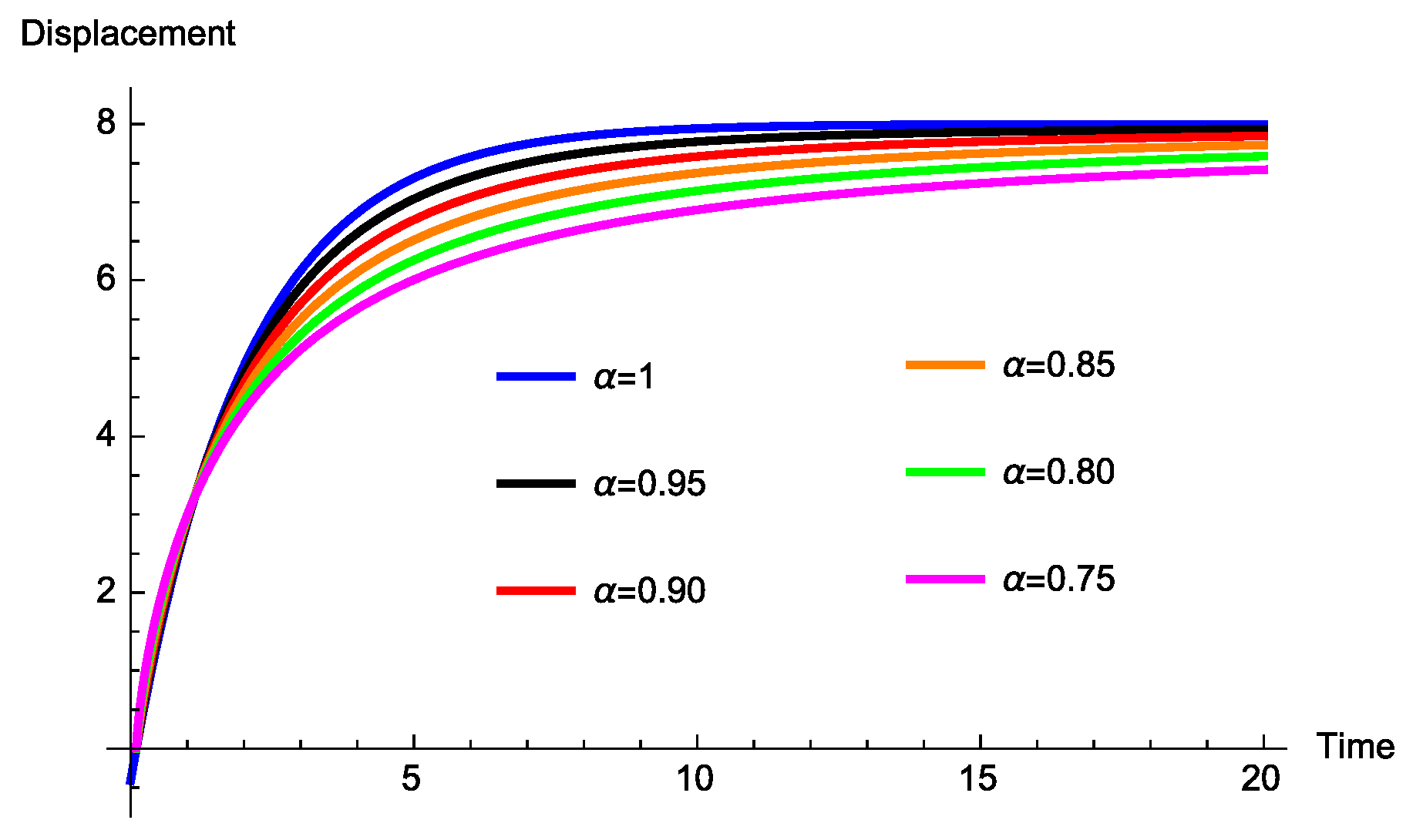
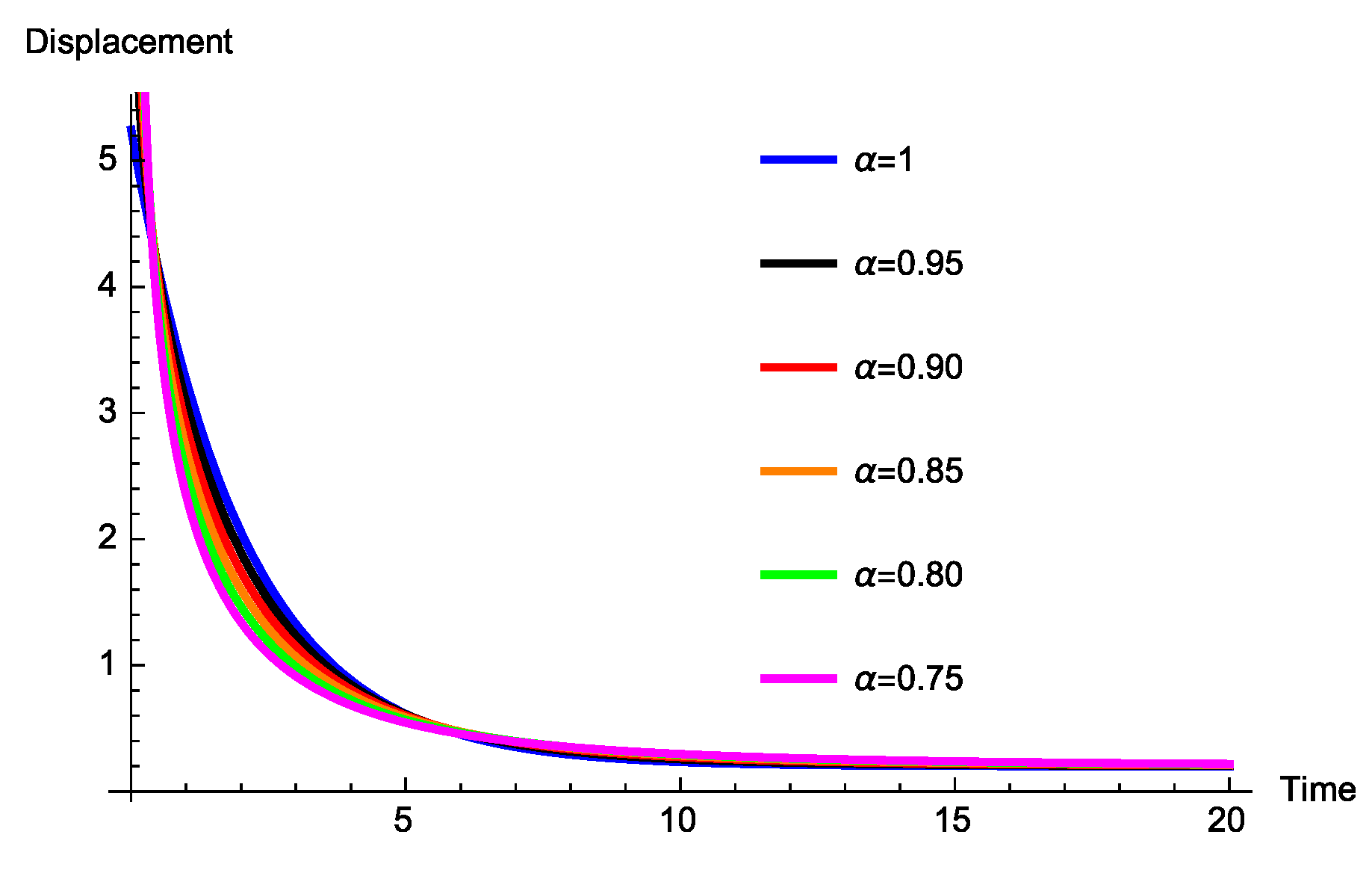
3.1.1. Absence of Mass

We consider the following spring-damper equation described by the Liouville–Caputo left generalized fractional derivative:

$$\frac{\beta }{{\sigma }^{1-\alpha }}{D}_c^{\alpha ,\rho }x\left(t\right)+kx\left(t\right)=u\left(t\right).$$

(9)

In the following theorem, we describe the procedure to obtain the analytical solution of the fractional spring-damper equation.

Theorem 1.

Under initial boundary condition $x\left(a\right)=\eta$ and considering the source term as v, the fractional spring-damper equation described by the Liouville–Caputo left generalized fractional derivative (9) is described by the following expression:

$$x\left(t\right)=\eta E_{\alpha }\left(\lambda {\left(\frac{t^{\rho }-a^{\rho }}{\rho }\right)}^{\alpha }\right)+{\int }_a^t{\left(\frac{t^{\rho }-s^{\rho }}{\rho }\right)}^{\alpha -1}{E}_{\alpha ,\alpha }\left(\lambda {\left(\frac{t^{\rho }-s^{\rho }}{\rho }\right)}^{\alpha }\right)u\left(s\right)\frac{ds}{s^{1-\rho }}.$$

(10)

where $\lambda =-\frac{k{\sigma }^{1-\alpha }}{\beta }$ and the exogenous input is given by $u\left(t\right)=\frac{{\sigma }^{1-\alpha }v\left(t\right)}{\beta }$.

Proof. 

Let $\lambda =-\frac{k{\sigma }^{1-\alpha }}{\beta }$ and the exogenous input $u\left(t\right)=\frac{{\sigma }^{1-\alpha }v\left(t\right)}{\beta }$. This follows the following fractional differential equation:

$$D_c^{\alpha ,\rho }=\lambda x\left(t\right)+u\left(t\right).$$

(11)

We notice that the fractional differential Equation (11) is a linear fractional differential equation described by the Liouville–Caputo generalized fractional derivative. The solution is obtained by applying the $\rho$-Laplace transform. $\overline{x}$ represents the usual Laplace transform of the function x, and $\overline{u}$ represents the usual Laplace transform of the input function u. This yields:

$$\begin{array}{ccc}\hfill s^{\alpha }\overline{x}\left(s\right)-s^{\alpha }\eta & =& \lambda \overline{x}\left(s\right)+\overline{u}\left(s\right),\hfill \\ \hfill s^{\alpha }\overline{x}\left(s\right)-\lambda \overline{x}\left(s\right)& =& s^{\alpha }\eta +\overline{u}\left(s\right),\hfill \\ \hfill \overline{x}\left(s\right)& =& \frac{s^{\alpha -1}\eta }{s^{\alpha }-\lambda }+\frac{\overline{u}\left(s\right)}{s^{\alpha }-\lambda }.\hfill \end{array}$$

(12)

Inverting Equation (12), we obtain the analytical solution of the fractional differential equation expressed by Equation (9) in the following form:

$$x\left(t\right)=\eta E_{\alpha }\left(\lambda {\left(\frac{t^{\rho }-a^{\rho }}{\rho }\right)}^{\alpha }\right)+{\int }_a^t{\left(\frac{t^{\rho }-s^{\rho }}{\rho }\right)}^{\alpha -1}{E}_{\alpha ,\alpha }\left(\lambda {\left(\frac{t^{\rho }-s^{\rho }}{\rho }\right)}^{\alpha }\right)u\left(s\right)\frac{ds}{s^{1-\rho }}.$$

(13)

 □

Let us show some special cases of the fractional spring-damper-equation. Let the exogenous input converge to a constant source term $u_0$. Using Theorem 1, the solution of the fractional spring-damper equation is given by:

$$x\left(t\right)=\left[\eta +\frac{u_0\beta }{k{\sigma }^{1-\alpha }}\right]E_{\alpha }\left(-\frac{k{\sigma }^{1-\alpha }}{\beta }{\left(\frac{t^{\rho }-a^{\rho }}{\rho }\right)}^{\alpha }\right)-\frac{u_0\beta }{k{\sigma }^{1-\alpha }}.$$

(14)

We observe that when exogenous input u converges to $u_0$ and t converges to infinity under the assumption that $\lambda \le 0$, the solution of the fractional spring-damper converges to $\frac{u_0}{\lambda }=\frac{u_0\beta }{k{\sigma }^{1-\alpha }}$, as well. That is, the fractional spring-damper system described by the Liouville–Caputo left generalized fractional derivative satisfies the property “converging-input-converging-state” [24]. The behaviors of the analytical solution of the fractional spring-damper equation for different values of the orders $\alpha$, $a=0$, $\eta =1$, and $\rho =1$ are depicted in Figure 1.

We can observe as well that with the orders $\alpha =1$, $a=0$, and $\rho =1$, we recover the analytical solution of the classical spring-damper system represented by the following expression:

$$x\left(t\right)=\left[\eta +\frac{u_0\beta }{k}\right]exp\left(-\frac{k}{\beta }t\right)-\frac{u_0\beta }{k}.$$

(15)

The second case considers the unforced fractional spring-damper system defined by the following equation:

$$\frac{\beta }{{\sigma }^{1-\alpha }}{D}_c^{\alpha ,\rho }x\left(t\right)+kx\left(t\right)=0.$$

(16)

The solution of Equation (16) is given by:

$$x\left(t\right)=\eta E_{\alpha }\left(-\frac{k{\sigma }^{1-\alpha }}{\beta }{\left(\frac{t^{\rho }-a^{\rho }}{\rho }\right)}^{\alpha }\right).$$

(17)

In other words, the trivial solution of the unforced fractional spring-damper defined by Equation (16) is asymptotically stable [25]. The behaviors of the analytical solution of the unforced fractional spring-damper equation for different values of the orders $\alpha$, $a=0$, $\eta =1$, and $\rho =1$ are depicted in Figure 2.

The third case consider an exogenous input sinusoidal. In other words, we consider $u\left(t\right)=u_{0}cos\left(wt\right)$; thus, the fractional spring-damper equation is represented by:

$$\frac{\beta }{{\sigma }^{1-\alpha }}{D}_c^{\alpha ,\rho }x\left(t\right)+kx\left(t\right)=u_{0}cos\left(wt\right).$$

(18)

Under Theorem 1, the analytical solution of the fractional spring-damper equation is described by:

$$x\left(t\right)=\eta E_{\alpha }\left(\lambda {\left(\frac{t^{\rho }-a^{\rho }}{\rho }\right)}^{\alpha }\right)+u_0{\int }_a^t{\left(\frac{t^{\rho }-s^{\rho }}{\rho }\right)}^{\alpha -1}{E}_{\alpha ,\alpha }\left(\lambda {\left(\frac{t^{\rho }-s^{\rho }}{\rho }\right)}^{\alpha }\right)cos\left(ws\right)\frac{ds}{s^{1-\rho }}.$$

(19)

The behaviors of the analytical solution of the fractional spring-damper Equation (19) under the sinusoidal source term, for different values of $\alpha$, $a=0$, $\eta =1$, and $\rho =1$ are depicted in Figure 3.

In the case $\alpha =1$, $a=0$, and $\rho =1$, we recover the analytical solution of the classical spring-damper system represented by the following expression:

$$x\left(t\right)=\eta exp\left(-\frac{k}{\beta }t\right)+u_0{\int }_0^{t}exp\left(-\frac{k}{\beta }\left(t-s\right)\right)cos\left(ws\right)ds.$$

(20)

3.1.2. Absence of the Spring Coefficient

We obtain the analytical solution of the fractional mass-damper equation ($\beta =0$) described by the Liouville–Caputo left generalized fractional derivative. The following equation characterizes the fractional differential equation under consideration:

$$\frac{m}{{\sigma }^{2(1-\alpha ),\rho }}{D}_c^{2\alpha ,\rho }x\left(t\right)+kx\left(t\right)=u\left(t\right).$$

(21)

Let $\lambda =-\frac{k{\sigma }^{2(1-\alpha ),\rho }}{m}$, $u\left(t\right)=\frac{v\left(t\right){\sigma }^{2(1-\alpha ),\rho }}{m}$, and the initial boundary condition defined by $x\left(0\right)=\eta .$

Theorem 2.

The analytical solution of the fractional mass-damper equation described by the Liouville–Caputo left generalized fractional derivative Equation (21) is represented by the following expression:

$$x\left(t\right)=\eta E_{2\alpha }\left(\lambda {\left(\frac{t^{\rho }-a^{\rho }}{\rho }\right)}^{2\alpha }\right)+{\int }_a^t{\left(\frac{t^{\rho }-s^{\rho }}{\rho }\right)}^{2\alpha -1}{E}_{2\alpha ,2\alpha }\left(\lambda {\left(\frac{t^{\rho }-s^{\rho }}{\rho }\right)}^{2\alpha }\right)u\left(s\right)\frac{ds}{s^{1-\rho }}.$$

(22)

Proof. 

Let $\lambda =-\frac{k{\sigma }^{2(1-\alpha ),\rho }}{m}$; the initial boundary condition is $x\left(a\right)=\eta$, and the exogenous input $u\left(t\right)=\frac{{\sigma }^{2(1-\alpha ),\rho }v\left(t\right)}{m}$. We have the following fractional differential equation:

$$D_c^{2\alpha ,\rho }=\lambda x\left(t\right)+u\left(t\right).$$

(23)

The solution is obtained after the application of the $\rho$-Laplace transform. Let $\overline{x}$ represent the usual Laplace transform of the function x and $\overline{u}$ represent the usual Laplace transform of the exogenous input u. We have:

$$\begin{array}{ccc}\hfill s^{2\alpha }\overline{x}\left(s\right)-s^{2\alpha }\eta & =& \lambda \overline{x}\left(s\right)+\overline{u}\left(s\right),\hfill \\ \hfill s^{2\alpha }\overline{x}\left(s\right)-\lambda \overline{x}\left(s\right)& =& s^{2\alpha }\eta +\overline{u}\left(s\right),\hfill \\ \hfill \overline{x}\left(s\right)& =& \frac{s^{2\alpha -1}\eta }{s^{2\alpha }-\lambda }+\frac{\overline{u}\left(s\right)}{s^{2\alpha }-\lambda }.\hfill \end{array}$$

(24)

We apply the inverse of the $\rho$-Laplace transform to both sides of Equation (24), and we obtain the analytical solution of the fractional differential equation expressed by Equation (23) in the following form:

$$x\left(t\right)=\eta E_{2\alpha }\left(\lambda {\left(\frac{t^{\rho }-a^{\rho }}{\rho }\right)}^{2\alpha }\right)+{\int }_a^t{\left(\frac{t^{\rho }-s^{\rho }}{\rho }\right)}^{2\alpha -1}{E}_{2\alpha ,2\alpha }\left(\lambda {\left(\frac{t^{\rho }-s^{\rho }}{\rho }\right)}^{2\alpha }\right)u\left(s\right)\frac{ds}{s^{1-\rho }}.$$

(25)

 □

Let us show some special cases of the fractional mass-damper equation. Let the exogenous input converge to a constant source term $u_0$. Using Theorem 2, the solution of the fractional mass-damper equation described by the Liouville–Caputo left generalized fractional derivative is given by:

$$x\left(t\right)=\left[\eta -\frac{u_{0}m}{k{\sigma }^{2(1-\alpha ),\rho }}\right]E_{2\alpha }\left(-\frac{k{\sigma }^{2(1-\alpha ),\rho }}{m}{\left(\frac{t^{\rho }-a^{\rho }}{\rho }\right)}^{2\alpha }\right)+\frac{u_{0}m}{k{\sigma }^{2(1-\alpha ),\rho }}.$$

(26)

Let the exogenous input u converge to $u_0$, as t converges to infinity. Under the assumption $\lambda \le 0$, the solution of the fractional mass damper described by the Liouville–Caputo left generalized fractional derivative converges to $\frac{u_0}{\lambda }=\frac{u_0\beta }{k{\sigma }^{1-\alpha }}$, as well. That is, the fractional mass-damper system satisfies the property converging-input-converging-state [24].

The behaviors of the analytical solution of the fractional mass-damper equation for different values of the orders $\alpha$, $a=0$, $\eta =1$, and $\rho =1$ are depicted in Figure 4.

As in the previous section, we can observe that when the orders $\alpha =1$, $a=0$ and $\rho =1$, we recover the analytical solution of the classical mass-damper system represented in the following expression:

$$x\left(t\right)=\left[\eta -\frac{u_{0}m}{k}\right]cos\left(\frac{k}{\beta }t\right)-\frac{u_{0}m}{k}.$$

(27)

Let the unforced fractional mass-damper equation be represented by the following equation:

$$\frac{m}{{\sigma }^{2(1-\alpha ),\rho }}{D}_c^{2\alpha ,\rho }x\left(t\right)+kx\left(t\right)=0.$$

(28)

Considering Theorem 2, we obtain the following solution:

$$x\left(t\right)=\left[\eta -\frac{u_{0}m}{k{\sigma }^{2(1-\alpha ),\rho }}\right]E_{2\alpha }\left(-\frac{k{\sigma }^{2(1-\alpha ),\rho }}{m}{\left(\frac{t^{\rho }-a^{\rho }}{\rho }\right)}^{2\alpha }\right).$$

(29)

The trivial solution of the unforced fractional mass-damper defined by Equation (28) is asymptotically stable. The behaviors of the analytical solution of the unforced fractional mass-damper equation for different values of $\alpha$, $a=0$, $\eta =1$, and $\rho =1$ are depicted in Figure 5.

Considering the exogenous input $u\left(t\right)=u_{0}cos\left(wt\right)$, the fractional mass damper equation is represented by:

$$\frac{m}{{\sigma }^{2(1-\alpha ),\rho }}{D}_c^{2\alpha ,\rho }x\left(t\right)+kx\left(t\right)=u_{0}cos\left(wt\right).$$

(30)

Using Theorem 2, the analytical solution is expressed in the following form:

$$x\left(t\right)=\eta E_{2\alpha }\left(\lambda {\left(\frac{t^{\rho }-a^{\rho }}{\rho }\right)}^{2\alpha }\right)+u_0{\int }_a^t{\left(\frac{t^{\rho }-s^{\rho }}{\rho }\right)}^{2\alpha -1}{E}_{2\alpha ,2\alpha }\left(\lambda {\left(\frac{t^{\rho }-s^{\rho }}{\rho }\right)}^{2\alpha }\right)cos\left(ws\right)\frac{ds}{s^{1-\rho }}.$$

(31)

The behaviors of the analytical solution of the fractional mass-damper Equation (31) for different values of $\alpha$, $a=0$, $\eta =1$, and $\rho =1$ are depicted in Figure 6.

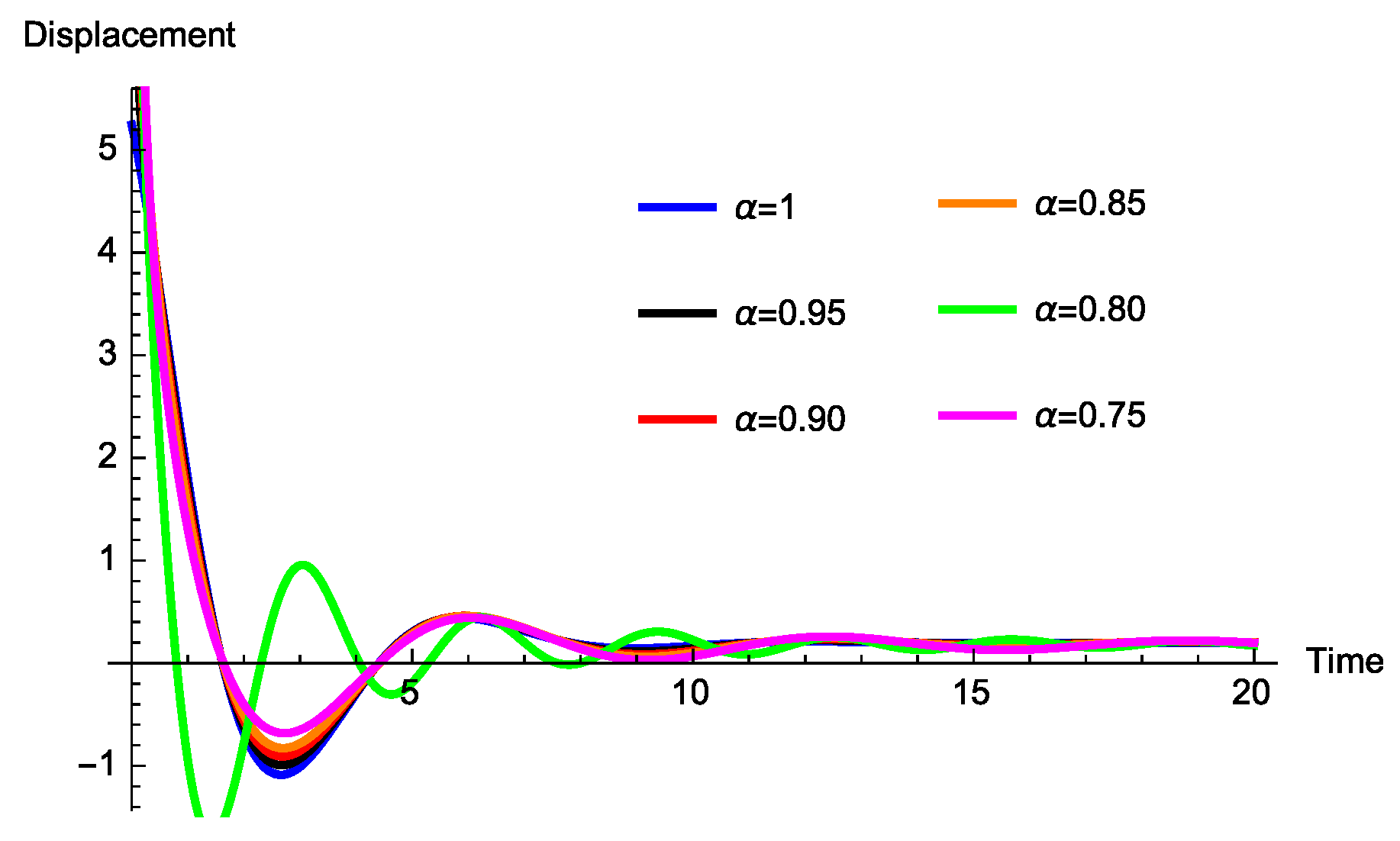
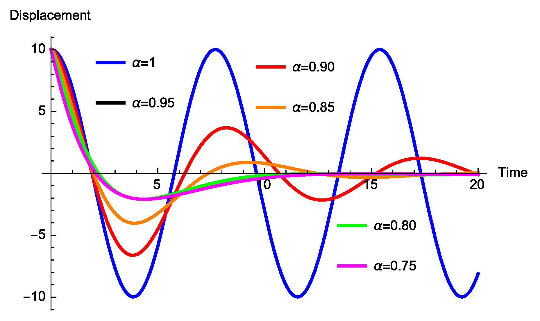
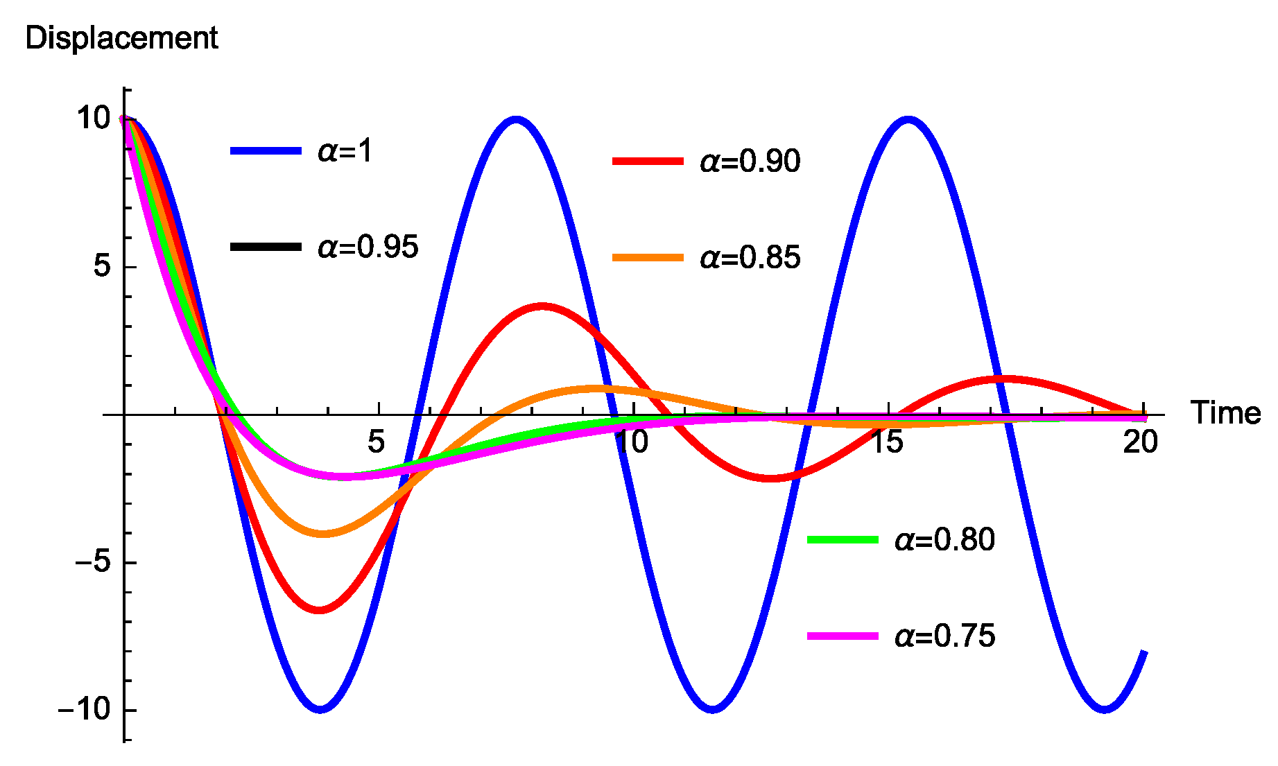
3.1.3. In the Presence of Mass and Spring Coefficients

We obtain the analytical solution of the fractional mass-spring-damper equation described by the Liouville–Caputo left generalized fractional derivative. The fractional differential equation under consideration is described by:

$$\frac{m}{{\sigma }^{2(1-\alpha ),\rho }}{D}_c^{2\alpha ,\rho }x\left(t\right)+\frac{\beta }{{\sigma }^{1-\alpha }}{D}_c^{\alpha ,\rho }x\left(t\right)+kx\left(t\right)=u\left(t\right).$$

(32)

We consider $\kappa =\frac{m}{{\sigma }^{2(1-\alpha ),\rho }}$, $b=\frac{\beta }{{\sigma }^{1-\alpha }}$, and $c=k$, and the exogenous input is null $u=0$. Equation (32) can be rewritten in the following form:

$$\kappa D_c^{2\alpha ,\rho }x\left(t\right)+b{D}_c^{\alpha ,\rho }x\left(t\right)+cx\left(t\right)=0.$$

(33)

Applying the $\rho$-Laplace transform to both sides of Equation (33), it follows that:

$$\begin{array}{ccc}\hfill \kappa s^{2\alpha }\overline{x}\left(s\right)-\kappa s^{2\alpha -1}\eta +b{s}^{\alpha }\overline{x}\left(s\right)-b{s}^{\alpha -1}\eta +c\overline{x}\left(s\right)& =& 0,\hfill \\ \hfill \kappa s^{2\alpha -1}\eta +b{s}^{\alpha -1}\eta & =& \overline{x}\left(s\right)\left(\kappa s^{2\alpha }+b{s}^{\alpha }+c\right),\hfill \\ \hfill \frac{\kappa s^{2\alpha -1}\eta }{\kappa s^{2\alpha }+b{s}^{\alpha }+c}+\frac{b{s}^{\alpha -1}\eta }{\kappa s^{2\alpha }+b{s}^{\alpha }+c}& =& \overline{x}\left(s\right).\hfill \end{array}$$

(34)

We obtain the analytical solution of the fractional mass-spring-damper equation without input by applying the inverse of the $\rho$-Laplace transform to both sides of Equation (35). The analytical solution is obtained using series decomposition:

$$\begin{array}{ccc}\hfill x\left(t\right)& =& \sum _{k=0}^{\infty }\frac{{(-1)}^k}{k!}{\left(\frac{b}{\kappa }\right)}^k\eta {\left(\frac{t^{\rho }-a^{\rho }}{\rho }\right)}^{k\alpha }{E}_{2\alpha ,1-k\alpha }^{\left(k\right)}\left(-\frac{c}{\kappa }{\left(\frac{t^{\rho }-a^{\rho }}{\rho }\right)}^{2\alpha }\right)\hfill \\ & +& \sum _{k=0}^{\infty }\frac{{(-1)}^k}{k!}{\left(\frac{b}{\kappa }\right)}^{k+1}\eta {\left(\frac{t^{\rho }-a^{\rho }}{\rho }\right)}^{(k+1)\alpha }{E}_{2\alpha ,1-(k-1)\alpha }^{\left(k\right)}\left(-\frac{c}{\kappa }{\left(\frac{t^{\rho }-a^{\rho }}{\rho }\right)}^{2\alpha }\right).\hfill \end{array}$$

(35)

The behaviors of the analytical solution of the fractional mass-spring-damper Equation (35) for different values of $\alpha$, $a=0$, $\eta =1$ and $\rho =1$ are depicted in Figure 7.

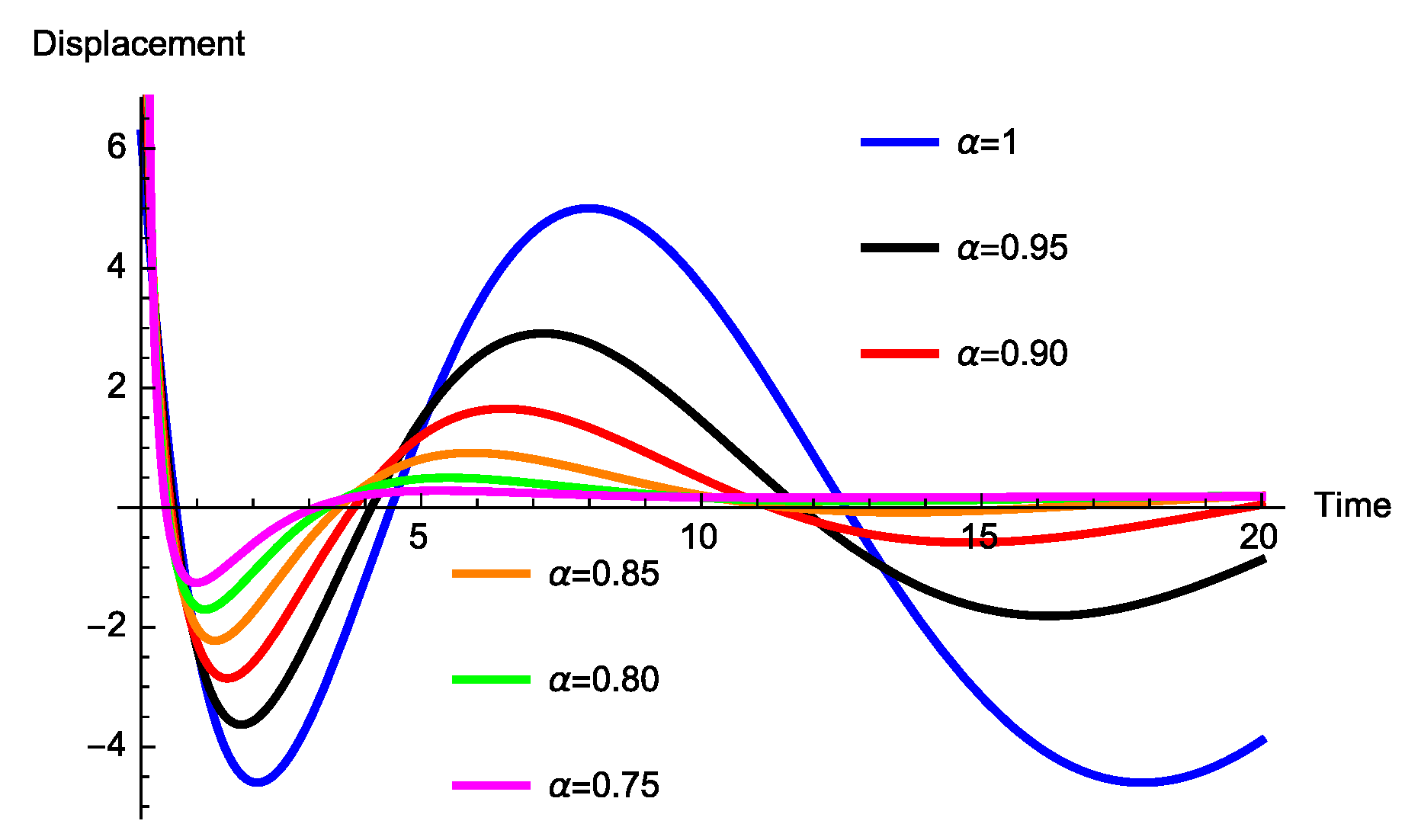
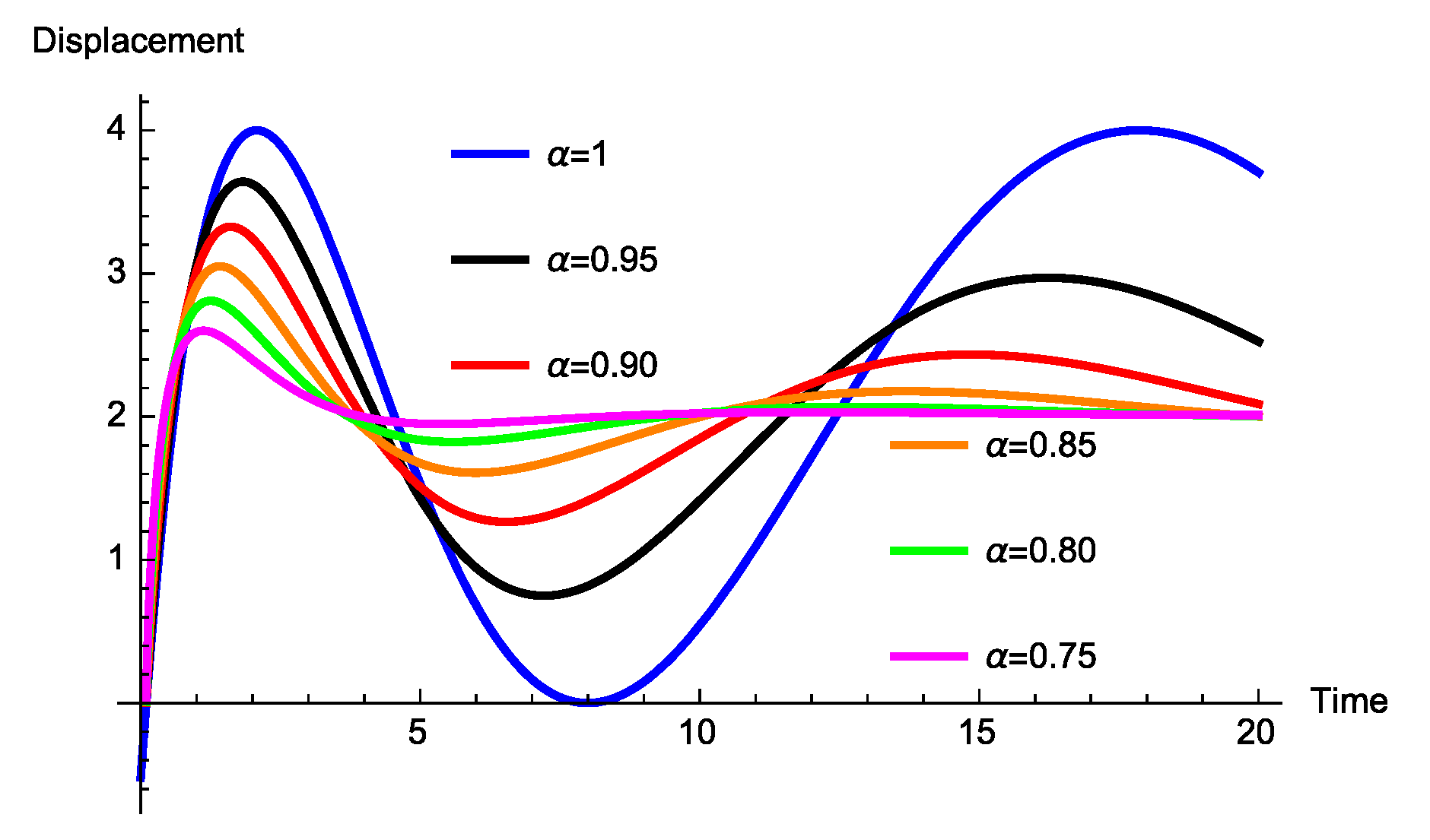
3.2. Left Generalized Fractional Derivative

Now, we consider the mass-spring-damper equation described by the left generalized fractional derivative defined by:

$$\frac{m}{{\sigma }^{2(1-\alpha ),\rho }}{D}^{2\alpha ,\rho }x\left(t\right)+\frac{\beta }{{\sigma }^{1-\alpha }}{D}^{\alpha ,\rho }x\left(t\right)+kx\left(t\right)=u\left(t\right).$$

(36)

We investigate the analytical solutions of Equation (36) when the Liouville–Caputo left generalized fractional derivative is replaced by the left generalized fractional derivative. We consider three cases: the absence of mass $m=0$, the absence of a spring $\beta =0$, and the complete fractional mass-spring-damper system.

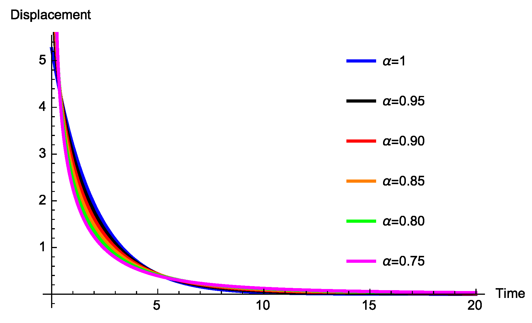
3.2.1. Absence of Mass

The following equation describes the fractional differential equation under consideration:

$$\frac{\beta }{{\sigma }^{1-\alpha }}{D}^{\alpha ,\rho }x\left(t\right)+kx\left(t\right)=u\left(t\right).$$

(37)

In the following theorem, we describe the analytical solution of the fractional spring-damper equation.

Theorem 3.

Under boundary condition $\left(I^{1-\alpha ,\rho }x\right)\left(a\right)=\eta$ and the source term v, the analytical solution of the fractional spring damper Equation (37) is described by the following expression:

$$x\left(t\right)=\eta {\left(\frac{t^{\rho }-a^{\rho }}{\rho }\right)}^{\alpha -1}{E}_{\alpha ,\alpha }\left(\lambda {\left(\frac{t^{\rho }-a^{\rho }}{\rho }\right)}^{\alpha }\right)+{\int }_a^t{\left(\frac{t^{\rho }-s^{\rho }}{\rho }\right)}^{\alpha -1}{E}_{\alpha ,\alpha }\left(\lambda {\left(\frac{t^{\rho }-s^{\rho }}{\rho }\right)}^{\alpha }\right)u\left(s\right)\frac{ds}{s^{1-\rho }},$$

(38)

where $\lambda =-\frac{k{\sigma }^{1-\alpha }}{\beta }$ and the exogenous input $u\left(t\right)=\frac{{\sigma }^{1-\alpha }v\left(t\right)}{\beta }$.

Proof. 

Let the following fractional differential equation be described by the left generalized fractional derivative:

$$D^{\alpha ,\rho }=\lambda x\left(t\right)+u\left(t\right).$$

(39)

The solution of Equation (39) is obtained applying the $\rho$-Laplace transform. In this case, $\overline{x}$ represents the usual Laplace transform of the function x, and $\overline{u}$ represents the usual Laplace transform of the input function u. We obtain:

$$\begin{array}{ccc}\hfill s^{\alpha }\overline{x}\left(s\right)-\eta & =& \lambda \overline{x}\left(s\right)+\overline{u}\left(s\right),\hfill \\ \hfill s^{\alpha }\overline{x}\left(s\right)-\lambda \overline{x}\left(s\right)& =& \eta +\overline{u}\left(s\right),\hfill \\ \hfill \overline{x}\left(s\right)& =& \frac{\eta }{s^{\alpha }-\lambda }+\frac{\overline{u}\left(s\right)}{s^{\alpha }-\lambda }.\hfill \end{array}$$

(40)

Inverting Equation (40) using the inverse of the $\rho$-Laplace transform, we obtain the analytical solution of the fractional differential equation expressed by Equation (39). We have:

$$x\left(t\right)=\eta {\left(\frac{t^{\rho }-a^{\rho }}{\rho }\right)}^{\alpha -1}{E}_{\alpha ,\alpha }\left(\lambda {\left(\frac{t^{\rho }-a^{\rho }}{\rho }\right)}^{\alpha }\right)+{\int }_a^t{\left(\frac{t^{\rho }-s^{\rho }}{\rho }\right)}^{\alpha -1}{E}_{\alpha ,\alpha }\left(\lambda {\left(\frac{t^{\rho }-s^{\rho }}{\rho }\right)}^{\alpha }\right)u\left(s\right)\frac{ds}{s^{1-\rho }}.$$

(41)

 □

Let the exogenous input converge to a constant source term $u_0$. Using Theorem 1, the solution of the fractional spring-damper equation is given by:

$$x\left(t\right)=\eta {\left(\frac{t^{\rho }-a^{\rho }}{\rho }\right)}^{\alpha -1}{E}_{\alpha ,\alpha }\left(-\frac{k{\sigma }^{1-\alpha }}{\beta }{\left(\frac{t^{\rho }-a^{\rho }}{\rho }\right)}^{\alpha }\right)-\frac{u_0\beta }{k{\sigma }^{1-\alpha }}{E}_{\alpha }\left(-\frac{k{\sigma }^{1-\alpha }}{\beta }{\left(\frac{t^{\rho }-a^{\rho }}{\rho }\right)}^{\alpha }\right)+\frac{u_0\beta }{k{\sigma }^{1-\alpha }}.$$

(42)

When the exogenous input u converges to $u_0$ and t converges to infinity, under the assumption $\lambda \le 0$, the solution of the fractional spring-damper system converges to $\frac{u_0}{\lambda }=\frac{u_0\beta }{k{\sigma }^{1-\alpha }}$. Thus, the fractional spring-damper system satisfies the property converging-input-converging-state [24]. The behaviors of the analytical solution of the fractional spring-damper equation for several values of the orders $\alpha$, $a=0$, and $\eta =1$ are depicted in Figure 8.

For the unforced fractional spring-damper system, using Theorem 3, we obtain the following solution:

$$x\left(t\right)=\eta {\left(\frac{t^{\rho }-a^{\rho }}{\rho }\right)}^{\alpha -1}{E}_{\alpha ,\alpha }\left(-\frac{k{\sigma }^{1-\alpha }}{\beta }{\left(\frac{t^{\rho }-a^{\rho }}{\rho }\right)}^{\alpha }\right).$$

(43)

The trivial solution of the unforced fractional spring-damper defined by:

$$\frac{\beta }{{\sigma }^{1-\alpha }}{D}^{\alpha ,\rho }x\left(t\right)+kx\left(t\right)=0,$$

is Mittag–Leffler stable [25]. The behavior of the analytical solution of the unforced fractional spring-damper equation for several values of the orders $\alpha$, $a=0$, and $\eta =1$ is depicted in Figure 9.

When the exogenous input is sinusoidal, let $u\left(t\right)=u_{0}cos\left(wt\right)$, and the fractional spring-damper equation is represented by:

$$\frac{\beta }{{\sigma }^{1-\alpha }}{D}^{\alpha ,\rho }x\left(t\right)+kx\left(t\right)=u_{0}cos\left(wt\right).$$

(44)

Under Theorem 3, the analytical solution of the fractional spring-damper Equation (44) is described by:

$$x\left(t\right)=\eta {\left(\frac{t^{\rho }-a^{\rho }}{\rho }\right)}^{\alpha -1}{E}_{\alpha ,\alpha }\left(\lambda {\left(\frac{t^{\rho }-a^{\rho }}{\rho }\right)}^{\alpha }\right)+u_0{\int }_a^t{\left(\frac{t^{\rho }-s^{\rho }}{\rho }\right)}^{\alpha -1}{E}_{\alpha ,\alpha }\left(\lambda {\left(\frac{t^{\rho }-s^{\rho }}{\rho }\right)}^{\alpha }\right)cos\left(ws\right)\frac{ds}{s^{1-\rho }}.$$

(45)

The behaviors of the analytical solution of the fractional spring damper Equation (45) under the sinusoidal source term for several values of the orders $\alpha$, $a=0$, and $\eta =1$ are depicted in Figure 10.

3.2.2. Absence of the Spring Coefficient

We obtain the analytical solution of the fractional mass-damper equation described by the left generalized fractional derivative. The following equation defines the fractional differential equation when $\beta =0$:

$$\frac{m}{{\sigma }^{2(1-\alpha ),\rho }}{D}^{2\alpha ,\rho }x\left(t\right)+kx\left(t\right)=u\left(t\right).$$

(46)

For simplicity $\lambda =-\frac{k{\sigma }^{2(1-\alpha ),\rho }}{m}$, $u\left(t\right)=\frac{v\left(t\right){\sigma }^{2(1-\alpha ),\rho }}{m}$, and the initial condition is $\left(I^{1-\alpha ,\rho }x\right)\left(a\right)=\eta$. The main result is described in the following theorem.

Theorem 4.

The analytical solution of the fractional mass-damper equation described by the Caputo left generalized fractional derivative (46) is described by the following expression:

$$x\left(t\right)=\eta {\left(\frac{t^{\rho }-a^{\rho }}{\rho }\right)}^{2\alpha -1}{E}_{2\alpha ,2\alpha }\left(\lambda {\left(\frac{t^{\rho }-a^{\rho }}{\rho }\right)}^{2\alpha }\right)+{\int }_a^t{\left(\frac{t^{\rho }-s^{\rho }}{\rho }\right)}^{2\alpha -1}{E}_{2\alpha ,2\alpha }\left(\lambda {\left(\frac{t^{\rho }-s^{\rho }}{\rho }\right)}^{2\alpha }\right)u\left(s\right)\frac{ds}{s^{1-\rho }}.$$

(47)

Proof. 

After simplifications, we obtain the following fractional differential equation:

$$D^{2\alpha ,\rho }=\lambda x\left(t\right)+u\left(t\right).$$

(48)

The solution is obtained after the application of the $\rho$-Laplace transform. Let $\overline{x}$ represent the usual Laplace transform of the function x and $\overline{u}$ represent the usual Laplace transform of the exogenous input u; we obtain:

$$\begin{array}{ccc}\hfill s^{2\alpha }\overline{x}\left(s\right)-\eta & =& \lambda \overline{x}\left(s\right)+\overline{u}\left(s\right),\hfill \\ \hfill s^{2\alpha }\overline{x}\left(s\right)-\lambda \overline{x}\left(s\right)& =& \eta +\overline{u}\left(s\right),\hfill \\ \hfill \overline{x}\left(s\right)& =& \frac{\eta }{s^{2\alpha }-\lambda }+\frac{\overline{u}\left(s\right)}{s^{2\alpha }-\lambda }.\hfill \end{array}$$

(49)

Applying the inverse of the $\rho$-Laplace transform to both sides to Equation (49), we obtain the analytical solution of the fractional differential equation expressed by Equation (48). We have the solution defined by:

$$x\left(t\right)=\eta {\left(\frac{t^{\rho }-a^{\rho }}{\rho }\right)}^{2\alpha -1}{E}_{2\alpha ,2\alpha }\left(\lambda {\left(\frac{t^{\rho }-a^{\rho }}{\rho }\right)}^{2\alpha }\right)+{\int }_a^t{\left(\frac{t^{\rho }-s^{\rho }}{\rho }\right)}^{2\alpha -1}{E}_{2\alpha ,2\alpha }\left(\lambda {\left(\frac{t^{\rho }-s^{\rho }}{\rho }\right)}^{2\alpha }\right)u\left(s\right)\frac{ds}{s^{1-\rho }}.$$

(50)

 □

When the exogenous input converges to a constant source term $u_0$, the solution of the fractional mass-damper equation is obtained by using Theorem 4 in the following form:

$$x\left(t\right)=\eta {\left(\frac{t^{\rho }-a^{\rho }}{\rho }\right)}^{2\alpha -1}{E}_{2\alpha ,2\alpha }\left(\lambda {\left(\frac{t^{\rho }-a^{\rho }}{\rho }\right)}^{2\alpha }\right)-\frac{u_{0}m}{k{\sigma }^{2(1-\alpha ),\rho }}{E}_{2\alpha }\left(-\frac{k{\sigma }^{2(1-\alpha ),\rho }}{m}{\left(\frac{t^{\rho }-a^{\rho }}{\rho }\right)}^{2\alpha }\right)+\frac{u_{0}m}{k{\sigma }^{2(1-\alpha ),\rho }}.$$

(51)

When the exogenous input u converges to $u_0$ and t converges to infinity, the solution of the fractional mass-damper equation converges to $\frac{u_{0}m}{k{\sigma }^{2(1-\alpha ),\rho }}$. The fractional mass-damper system described by the left generalized fractional derivative satisfies the property converging-input-converging-state [24], and the behaviors of the analytical solution of the fractional mass-damper equation for several values of the order $\alpha$, $a=0$, and $\eta =1$ are depicted in Figure 11.

Now, we consider the unforced fractional mass-damper equation described by the left generalized fractional derivative represented by:

$$\frac{m}{{\sigma }^{2(1-\alpha ),\rho }}{D}^{2\alpha ,\rho }x\left(t\right)+kx\left(t\right)=0.$$

(52)

The analytical solution of the unforced fractional mass-damper equation is given by the following equation:

$$x\left(t\right)=\eta {\left(\frac{t^{\rho }-a^{\rho }}{\rho }\right)}^{2\alpha -1}{E}_{2\alpha ,2\alpha }\left(\lambda {\left(\frac{t^{\rho }-a^{\rho }}{\rho }\right)}^{2\alpha }\right).$$

(53)

The trivial solution of the unforced fractional mass-damper defined by Equation (52) is Mittag–Leffler stable. The behaviors of the analytical solution of the unforced fractional mass-damper equation described by the left generalized fractional derivative for several values of the orders $\alpha$, $a=0$, and $\eta =1$ are depicted in Figure 12.

Considering the exogenous input $u\left(t\right)=u_{0}cos\left(wt\right)$, the fractional mass-damper equation is represented by:

$$\frac{m}{{\sigma }^{2(1-\alpha ),\rho }}{D}^{2\alpha ,\rho }x\left(t\right)+kx\left(t\right)=u_{0}cos\left(wt\right).$$

(54)

It follows from Theorem 4 that the analytical solution of the fractional mass-damper equation is expressed in the following form:

$$x\left(t\right)=\eta {\left(\frac{t^{\rho }-a^{\rho }}{\rho }\right)}^{2\alpha -1}{E}_{2\alpha ,2\alpha }\left(\lambda {\left(\frac{t^{\rho }-a^{\rho }}{\rho }\right)}^{2\alpha }\right)+u_0{\int }_a^t{\left(\frac{t^{\rho }-s^{\rho }}{\rho }\right)}^{2\alpha -1}{E}_{2\alpha ,2\alpha }\left(\lambda {\left(\frac{t^{\rho }-s^{\rho }}{\rho }\right)}^{2\alpha }\right)cos\left(ws\right)\frac{ds}{s^{1-\rho }}.$$

(55)

The behaviors of the analytical solution of the fractional mass-damper equation given by Equation (53) for several values of the order $\alpha$, $a=0$, and $\eta =1$ are depicted in Figure 13.

4. Conclusions

In this paper, we investigated the analytical solution of the fractional mass-spring-damper equation described by the Caputo generalized fractional derivative and the left generalized fractional derivative. The converging-input converging-state of the fractional mass-damper and the fractional spring-damper were discussed. We also addressed the Mittag–Leffler stability of the unforced fractional mass-damper and the unforced fractional spring-damper. The present manuscript contributes to the application of fractional calculus in real-life problem. Here, we proved that the generalized fractional derivatives are an excellent compromise to study the behaviors of the mass-spring-damper systems.

References

1. Morales-Delgado, V.F.; Gómez-Aguilar, J.F.; Taneco-Hernández, M.A.; Escobar-Jiménez, R.F. A novel fractional derivative with variable- and constant-order applied to a mass-spring-damper system. Eur. Phys. J. Plus 2018, 133, 78. [Google Scholar] [CrossRef]
2. Hristov, J. A transient flow of a non-Newtonian fluid modelled by a mixed time-space derivative: An improved integral-balance approach. In Mathematical Methods in Engineering; Springer: Berlin, Germany, 2019; pp. 153–174. [Google Scholar]
3. Sheikh, N.A.; Ali, F.; Saqib, M.; Khan, I.; Jan, S.A.; Alshomrani, A.S.; Alghamdi, M.S. Comparison and analysis of the Atangana–Baleanu and Caputo–Fabrizio fractional derivatives for generalized Casson fluid model with heat generation and chemical reaction. Results Phys. 2017, 7, 789–800. [Google Scholar] [CrossRef]
4. Gómez-Aguilar, J.F.; Rosales-García, J.J.; Bernal-Alvarado, J.J.; Córdova-Fraga, T.; Gúzman-Cabrera, R. Fractional mechanical oscillators. Rev. Mex. Fís. 2012, 58, 348–352. [Google Scholar]
5. Iyiola, O.S.; Zaman, F.D. A fractional diffusion equation model for cancer tumor. AIP Adv. 2014, 4, 107121. [Google Scholar] [CrossRef]
6. Kumar, S.; Kumar, D.; Singh, J. Numerical computation of fractional Black–Scholes equation arising in financial market. Egyp. J. Basic Appl. Sci. 2014, 1, 177–183. [Google Scholar] [CrossRef]
7. Yavuz, M.; Özdemir, N. A different approach to the European option pricing model with new fractional operator. Math. Model. Nat. Phenom. 2018, 13, 1–12. [Google Scholar] [CrossRef]
8. Gómez-Aguilar, J.F.; Rosales-García, J.J.; Guía-Calderón, M.; Razo-Hernández, J.R. Fractional RC and LC electrical circuits. Ing. Investig. Tecnol. 2014, 15, 311–319. [Google Scholar]
9. Sene, N. Analytical solutions of Hristov diffusion equations with non-singular fractional derivatives. Chaos 2019, 29, 023112. [Google Scholar] [CrossRef]
10. Hristov, J. Approximate solutions to fractional subdiffusion equations. Eur. Phys. J. Spec. Top. 2011, 193, 229–243. [Google Scholar] [CrossRef] [Green Version]
11. Hristov, J. On the Atangana–Baleanu derivative and its relation to the fading memory concept: The diffusion equation formulation. In Trends in Theory and Applications of Fractional Derivatives with Mittag–Leffler Kernel; Springer: Berlin, Germany, 2019; pp. 1–22. [Google Scholar]
12. Sene, N. Stokes’ first problem for heated flat plate with Atangana–Baleanu fractional derivative. Chaos Solitons Fractals 2018, 117, 68–75. [Google Scholar] [CrossRef]
13. Sene, N.; Fall, A.N. Homotopy Perturbation ρ-Laplace Transform Method and Its Application to the Fractional Diffusion Equation and the Fractional Diffusion–Reaction Equation. Fract. Frac. 2019, 3, 14. [Google Scholar] [CrossRef]
14. Sene, N. Solutions of fractional diffusion equations and Cattaneo–Hristov diffusion model. Int. J. Anal. Appl. 2019, 17, 191–207. [Google Scholar]
15. Hristov, J. Fourth-order fractional diffusion model of thermal grooving: Integral approach to approximate closed form solution of the Mullins model. Math. Model. Nat. Phenom. 2018, 13, 1–6. [Google Scholar] [CrossRef]
16. Hristov, J. The heat radiation diffusion equation: Explicit analytical solutions by improved integral-balance method. Therm. Sci. 2018, 22, 777–788. [Google Scholar] [CrossRef] [Green Version]
17. Gómez-Aguilar, J.F.; Yépez-Martínez, H.; Calderón-Ramón, C.; Cruz-Orduña, I.; Eecobar-Jiménez, R.F.; Olivares-Peregrino, V.H. Modeling of a Mass-Spring-Damper System by Fractional Derivatives with and without a Singular Kernel. Entropy 2015, 17, 6289–6303. [Google Scholar] [CrossRef]
18. Ray, S.S.; Sahoo, S.; Das, S. Formulation and solutions of fractional continuously variable-order mass-spring damper systems controlled by viscoelastic and viscous-viscoelastic dampers. Adv. Mech. Eng. 2016, 8, 1–13. [Google Scholar] [CrossRef]
19. Gómez-Aguilar, J.F. Analytic solutions and numerical simulations of mass-spring and damper-spring systems described by fractional differential equations. Rom. J. Phys. 2015, 60, 311–323. [Google Scholar]
20. Escalante-Martínez, J.E.; Gómez-Aguilar, J.F.; Calderón-Ramón, C.; Morales-Mendoza, L.J.; Cruz-Orduna, I.; Laguna-Camacho, J.R. Experimental evaluation of viscous damping coefficient in the fractional underdamped oscillator. Adv. Mech. Eng. 2016, 8, 1–12. [Google Scholar] [CrossRef]
21. Fahd, J.; Abdeljawad, T. A modified Laplace transform for certain generalized fractional operators. Results Nonlinear Anal. 2018, 2, 88–98. [Google Scholar]
22. Katugampola, U.N. Theory and applications of fractional differential equations. Appl. Math. Comput. 2011, 218, 860–865. [Google Scholar]
23. Fahd, J.; Abdeljawad, T.; Baleanu, D. On the generalized fractional derivatives and their Caputo modification. J. Nonlinear Sci. Appl. 2017, 10, 2607–2619. [Google Scholar] [Green Version]
24. Sene, N. Fractional input stability for electrical circuits described by the Riemann–Liouville and the Caputo fractional derivatives. AIMS Math. 2019, 4, 147–165. [Google Scholar] [CrossRef]
25. Sene, N. Stability analysis of the generalized fractional differential equations with and without exogenous inputs. J. Nonlinear Sci. Appl. 2019, 12, 562–572. [Google Scholar] [CrossRef]
Figure 1. Numerical simulation for Equation (14) considering different values of α , arbitrarily chosen.
Fractalfract 03 00039 g001
Figure 2. Numerical simulation for Equation (17) considering different values of α , arbitrarily chosen.
Fractalfract 03 00039 g002
Figure 3. Numerical simulation for Equation (19) considering different values of α , arbitrarily chosen.
Fractalfract 03 00039 g003
Figure 4. Numerical simulation for Equation (26) considering different values of α , arbitrarily chosen.
Fractalfract 03 00039 g004
Figure 5. Numerical simulation for Equation (29) considering different values of α , arbitrarily chosen.
Fractalfract 03 00039 g005
Figure 6. Numerical simulation for Equation (31) considering different values of α , arbitrarily chosen.
Fractalfract 03 00039 g006
Figure 7. Numerical simulation for Equation (35) considering different values of α , arbitrarily chosen.
Fractalfract 03 00039 g007
Figure 8. Numerical simulation for Equation (42) considering different values of α , arbitrarily chosen.
Fractalfract 03 00039 g008
Figure 9. Numerical simulation for Equation (43) considering different values of α , arbitrarily chosen.
Fractalfract 03 00039 g009
Figure 10. Numerical simulation for Equation (45) considering different values of α , arbitrarily chosen.
Fractalfract 03 00039 g010
Figure 11. Numerical simulation for Equation (51) considering different values of α , arbitrarily chosen.
Fractalfract 03 00039 g011
Figure 12. Numerical simulation for Equation (53) considering different values of α , arbitrarily chosen.
Fractalfract 03 00039 g012
Figure 13. Numerical simulation for Equation (55) considering different values of α , arbitrarily chosen.
Fractalfract 03 00039 g013